This exercise in data analysis pins down a value of 1.8C for ECS.
Guest essay by Jeff L.
Introduction:
If the global climate debate between skeptics and alarmists were cooked down to one topic, it would be Equilibrium Climate Sensitivity to CO2 (ECS) , or how much will the atmosphere warm for a given increase in CO2 .
Temperature change as a function of CO2 concentration is a logarithmic function, so ECS is commonly expressed as X ° C per doubling of CO2. Estimates vary widely , from less than 1 ° C/ doubling to over 5 ° C / doubling. Alarmists would suggest sensitivity is on the high end and that catastrophic effects are inevitable. Skeptics would say sensitivity is on the low end and any changes will be non-catastrophic and easily adapted to.
All potential “catastrophic” consequences are based on one key assumption : High ECS ( generally > 3.0 ° C/ doubling of CO2). Without high sensitivity , there will not be large temperature changes and there will not be catastrophic consequences. As such, this is essentially the crux of the argument : if sensitivity is not high, all the “catastrophic” and destructive effects hypothesized will not happen. One could argue this makes ECS the most fundamental quantity to be understood.
In general, those who are supportive of the catastrophic hypothesis reach their conclusion based on global climate model output. As has been observed by many interested in the climate debate, over the last 15 + years, there has been a “pause” in global warming, illustrating that there are significant uncertainties in the validity of global climate models and the ECS associated with them.
There is a better alternative to using models to test the hypothesis of high ECS. We have temperature and CO2 data from pre-industrial times to present day. According to the catastrophic theory, the driver of all longer trends in modern temperature changes is CO2. As such, the catastrophic hypothesis is easily tested with the available data. We can use the CO2 record to calculate a series of synthetic temperature records using different assumed sensitivities and see what sensitivity best matches the observed temperature record.
The rest of this paper will explore testing the hypothesis of high ECS based on the observed data. I want to re-iterate the assumption of this hypothesis, which is also the assumption of the catastrophists position, that all longer term temperature change is driven by changes in CO2. I do not want to imply that I necessarily endorse this assumption, but I do want to illustrate the implications of this assumption. This is important to keep in mind as I will attribute all longer term temperature changes to CO2 in this analysis. I will comment at the end of this paper on the implications if this assumption is violated.
Data:
There are several potential datasets that could be used for the global temperature record. One of the longer and more commonly referenced datasets is HADCRUT4, which I have used for this study (plotted in fig. 1) The data may be found at the following weblink :
http://www.cru.uea.ac.uk/cru/data/temperature/HadCRUT4-gl.dat
I have used the annualized Global Average Annual Temperature anomaly from this data set. This data record starts in 1850 and goes to present, so we have 163 years of data. For the purposes on this analysis, the various adjustments that have been made to the data over the years will make very little difference to the best fit ECS. I will calculate what ECS best fits this temperature record, given the CO2 record.

Figure 1 : HADCRUT4 Global Average Annual Temperature Anomaly
The CO2 data set is from 2 sources. From 1959 to present, the Mauna Loa annual mean CO2 concentration is used. The data may be found at the following weblink :
ftp://aftp.cmdl.noaa.gov/products/trends/co2/co2_annmean_mlo.txt
For pre-1959, ice core data from Law Dome is used. The data may be found at the following weblink :
ftp://ftp.ncdc.noaa.gov/pub/data/paleo/icecore/antarctica/law/law_co2.txt
The Law Dome data record runs from 1832 to 1978. This is important for 2 reasons. First, and most importantly, it overlaps Mauna Loa data set. It can easily be seen in figure 2 that it is internally consistent with the Mauna Loa data set, thus providing higher confidence in the pre-Mauna Loa portion of the record. Second, the start of the data record pre-dates the start of the HADCRUT4 temperature record, allowing estimates of ECS to be tested against the entire HADCRUT4 temperature record. For the calculations that follow, a simple splice of the pre-1959 Law Dome data onto the Mauna Loa data was made , as the two data sets tie with little offset.

Figure 2 : Modern CO2 concentration record from Mauna Loa and Law Dome Ice Core.
Calculations:
From the above CO2 record, a set of synthetic temperature records can be constructed with various assumed ECS values. The synthetic records can then be compared to the observed data (HADCRUT4) and a determination of the best fit ECS can be made.
The equation needed for the calculation of the synthetic temperature record is as follows :
∆T = ECS* ln(C2/C1)) / ln(2)
where :
∆T = Change in temperature, ° C
ECS = Equilibrium Climate Sensitivity , ° C /doubling
C1 = CO2 concentration (PPM) at time 1
C2 = CO2 concentration (PPM) at time 2
For the purposes of this test of sensitivity, I set time 1 to 1850, the start of the HADCRUT4 temperature dataset. C1 at the same time from the Law Dome data set is 284.7 PPM. For each year from 1850 to 2013, I use the appropriate C2 value for that time and calculate ∆T with the formula above. To tie back to the HADCRUT4 data set, I use the HADCRUT4 temperature anomaly in 1850 ( -0.374 ° C) and add on the calculated ∆T value to create a synthetic temperature record.
ECS values ranging from 0.0 to 5.0 ° C /doubling were used to create a series of synthetic temperature records. Figure 3 shows the calculated synthetic records, labeled by their input ECS, as well as the observed HADCRUT4 data.

Figure 3: HADCRUT4 Observed data and synthetic temperature records for ECS values between 0.0 and 5.0 ° C / doubling. Where not labeled, synthetic records are at increments of 0.2 ° C / doubling. Warmer colors are warmer synthetic records.
From Figure 3, it is visually apparent that a ECS value somewhere close to 2.0 ° C/ doubling is a reasonable match to the observed data. This can be more specifically quantified by calculating the Mean Squared Error (MSE) of the synthetic records against the observed data. This is a “goodness of fit” measurement, with the minimum MSE representing the best fit ECS value. Figure 4 is a plot of MSE values for each ECS synthetic record.

Figure 4 : Mean Squared Error vs ECS values. A few ECS values of interest are labeled for further discussion
In plotting, the MSE values, a ECS value 1.8 ° C/ doubling is found to have the minimum MSE and thus is determined to be the best estimate of ECS based on the observed data over the last 163 years.
Discussion :
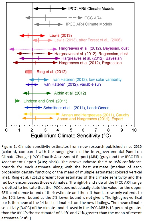
A comparison to various past estimates of ECS is made in figure 5. The base for figure 5 comes from the following weblink :
http://www.cato.org/sites/cato.org/files/wp-content/uploads/gsr_042513_fig1.jpg
See link for the original figure.

Figure 5 : Comparison of the results of this study (1.8) to other recent ECS estimates.
The estimate derived from this study agrees very closely with other recent studies. The gray line on figure 5 at a value of 2.0 represents the mean of 14 recent studies. Looking at the MSE curve in figure 4, 2.0 is essentially flat with 1.8 and would have a similar probability. This study further reinforces the conclusions of other recent studies which suggest climate sensitivity to CO2 is low relative to IPCC estimates .
The big difference with this study is that it is strictly based on the observed data. There are no models involved and only one assumption – that the longer period variation in temperature is driven by CO2 only. Given that the conclusion of a most likely sensitivity of 1.8 ° C / doubling is based on 163 years of observed data, the conclusion is likely to be quite robust.
A brief discussion of the assumption will now be made in light of the conclusion. The question to be asked is : If there are other factors affecting the long period trend of the observed temperature trend (there are many other potential factors, none of which will be discussed in this paper), what does that mean in terms of this best fit ECS curve ?
There are 2 options. If the true ECS is higher than 1.8, by definition , to match the observed data, there has to be some sort of negative forcing in the climate system pushing the temperature down from where it would be expected to be. In this scenario, CO2 forcing would be preventing the temperature trend from falling and is providing a net benefit.
The second option is the true ECS is lower than 1.8. In this scenario, also by definition, there has to be another positive forcing in the climate system pushing the temperature up to match the observed data. In this case CO2 forcing is smaller and poses no concern for detrimental effects.
For both of these options, it is hard to paint a picture where CO2 is going to be significantly detrimental to human welfare. The observed temperature and CO2 data over the last 163 years simply doesn’t allow for it.
Conclusion :
Based on data sets over the last 163 years, a most likely ECS of 1.8 ° C / doubling has been determined. This is a simple calculation based only on data , with no complicated computer models needed.
An ECS value of 1.8 is not consistent with any catastrophic warming estimates but is consistent with skeptical arguments that warming will be mild and non-catastrophic. At the current rate of increase of atmospheric CO2 (about 2.1 ppm/yr), and an ECS of 1.8, we should expect 1.0 ° C of warming by 2100. By comparison, we have experienced 0.86 ° C warming since the start of the HADCRUT4 data set. This warming is similar to what would be expected over the next ~ 100 years and has not been catastrophic by any measure.
For comparison of how unlikely the catastrophic scenario is, the IPCC AR5 estimate of 3.4 has an MSE error nearly as large as assuming that CO2 has zero effect on atmospheric temperature (see fig. 4).
There had been much discussion lately of how the climate models are diverging from the observed record over the last 15 years , due to “the pause”. All sorts of explanations have been posited by those supporting a high ECS value. The most obvious resolution is that the true ECS is lower, such as concluded in this paper. Note how “the pause” brings the observed temperature curve right to the 1.8 ECS synthetic record (see fig. 3). Given an ECS of 1.8, the global temperature is right where one would predict it should be. No convoluted explanations for “the pause” are needed with a lower ECS.
The high sensitivity values used by the IPCC , with their assumption that long term temperature trends are driven by CO2, are completely unsupportable based on the observed data. Along with that, all conclusions of “climate change” catastrophes are also completely unsupportable because they have the high ECS values the IPCC uses built into them (high ECS to get large temperature changes to get catastrophic effects).
Furthermore and most importantly, any policy changes designed to curb “climate change” are also unsupportable based on the data. It is assumed that the need for these policies is because of potential future catastrophic effects of CO2 but that is predicated on the high ECS values of the IPCC.
Files:
I have also attached a spreadsheet with all my raw data and calculations so anyone can easily replicate the work.
ECS Data (xlsx)
=============================================================
About Jeff:
I have followed the climate debate since the 90s. I was an early “skeptic” based on my geologic background – having knowledge of how climate had varied over geologic time, the fact that no one was talking about natural variation and natural cycles was an immediate red flag. The further I dug into the subject, the more I realized there were substantial scientific problems. The paper I am submitting is a paper I have wanted to write for years , as I did the basic calculations several years ago & realized there was no support in the observed data for high climate sensitivity.
@Doug Allen-If you think Willis thinks climate sensitivity is ~3, you haven’t been around or paying very much attention at all.
The 1.8 ECS would seem to be worst case given the period chosen, which is highly likely to have seen temperature increases anyway as we came out of the mini ice age around the time this data series started. While some of this is ironed out in the best fit exercise, one would think there is still an artificial lift given to the ECS here(?). The time period chosen is large enough to see 2+ cycles of natural factors of around 60 year periodicity (ENSO?) but not large enough to include a good sample of 100-200+ year cycles of which I believe there is at least one significant one. Interesting, but will have to read through more comments to understand the robustness of it. Appreciate the work.
alcheson says:
February 13, 2014 at 3:15 pm
Mosher says
“‘In general, those who are supportive of the catastrophic hypothesis reach their conclusion based on global climate model output.”
Wrong. Hansen for example relies on Paleo data.”
Really Mosh?
#######################
YES do not be stuck on stupid
http://blogs.plos.org/retort/2013/12/03/qa-with-james-hansen/
Q& A with Hansen
Q:At first glance there are a lot of messages in the paper that people could say they’ve heard before. We’ve heard before, obviously, that we need to reduce CO2 emissions. We’ve heard before that there’s a danger of moving the climate out of the conditions seen in the Holocene. How does your paper move those messages past what we’ve heard previously?
A: I think it’s more persuasive. It’s based fundamentally on observations, on studies of earth’s energy imbalance and the paleoclimate rather than on climate models. Although I’ve spent decades working on [climate models], I think there probably will remain for a long time major uncertainties, because you just don’t know if you have all of the physics in there. Some of it, like about clouds and aerosols, is just so hard that you can’t have very firm confidence. So yes, while you could say most of these [messages] you can find one place or another, but we’ve put the whole story together. The idea was not that we were producing a really new finding but rather that we were making a persuasive case for the judge.
############
https://www.skepticalscience.com/hansen-and-sato-2012-climate-sensitivity.html
“”These model-based studies provide invaluable insight into the functioning of the climate system, because it is possible to vary processes and parameters independently, thus examining the role and importance of different climate mechanisms. However, the model studies also make clear that the results vary substantially from one model to another, and experience of the past few decades suggests that models are not likely to converge to a narrow range in the near future.
Therefore there is considerable merit in also pursuing a complementary approach that estimates climate sensitivity empirically from known climate change and climate forcings.”
“”the empirical paleoclimate estimate of climate sensitivity is inherently more accurate than model-based estimates because of the difficulty of simulating cloud changes (NYTimes, 2012), aerosol changes, and aerosol effects on clouds.”
Dr. Nir Shaviv performed a somewhat more comprehensive analysis, and pointed out in
http://www.sciencebits.com/OnClimateSensitivity
“If the cosmic ray flux climate link is included in the radiation budget, averaging the different estimates for the sensitivity give a somewhat lower result…(Corresponding to ΔTx2=1.3±0.4°). Interestingly, this result is quite similar to the so called “black body” (i.e., corresponding to a climate system with feedbacks that tend to cancel each other).”
REPLY: and I call BS on your “wrong”
you havent read Hansen. See the comment above. Plus I’ve had the opportunity to listen to him and others on many occasions make the same argument.
Plus the IPCC charts show the same thing.
Hansen thinks the BEST argument is made from Paleo. He has written this on many occasions.
He thinks 3C will be catastrophic.
Look at the figures here Figure 3.
http://www.iac.ethz.ch/people/knuttir/papers/knutti08natgeo.pdf
NOTE: models do NOT present the long tails that some worry about. the instrumental period does
“If only Mosher et al would read & understand Dr. Hans Jelbring’s paper”
I’ll summarize it: lunatic.
“I am quite happy for them to use the ice core CO2/Temperature record to calculate ECS, as long as they use the atmospheric Dust levels as a proxy for aerosol forcing. Given that dust levels change by three orders of magnitude from warm to cold ages, with 1000 times more atmospheric dust in the ice ages when compared to the warmest parts of the record, they don’t use them
Any reconstruction that ignores the dust levels is completely and utterly bogus; but then you knew that Mosher.”
Doc, you should read Hansen’s Paper.
Look, you guys do STILL not get it.
Nic Lewis took an ACCEPTED paper and Improved it and the estimate went down
These approaches are filled with assumptions and uncertainty. You could take Hansens approach, take his LGM paper improve his method and argue for less than the 3C he found.
Some have.. they get to around 2.5C
It is FAR FAR FAR Better to accept the tools of your opponent, sharpen them, and use them against your opponents.
RichardLH says:
February 13, 2014 at 4:10 pm
Steven Mosher:
“Hansen for example relies on Paleo data.”
And he was SO right about how all this would play out wasn’t he?
###################
which part of logic dont you get.
The claim was made that high estimates from MODELS drove the CAGW storyline
Thats wrong.
the highest values come from studies of the instrumental period.
once folks ran a computer experiment that generated really high numbers
GAVIN SCHMIDT SHOT IT DOWN FOR CHRISTS SAKE.
http://www.realclimate.org/index.php/archives/2005/01/climatepredictionnet-climate-challenges-and-climate-sensitivity/
“Uncertainty in climate sensitivity is not going to disappear any time soon, and should therefore be built into assessments of future climate. However, it is not a completely free variable, and the extremely high end values that have been discussed in media reports over the last couple of weeks are not scientifically credible. ”
##############
Bottom line. As I said there are basically three approaches to deriving sensitivity. Models is ONE. The results from models tend to be TIGHTER than those from instruments or paleo.
The HIGHEST ESTIMATES do not come from models. The LOWEST estimates do not come from models.. in short models do very little to constrain the estimate.
Correlation is not causation comes to mind. Historically, as you go much further back then this analysis, temps and CO2 do not correlate well. In fact, in the historical record, CO2 lags temps.
Of course, our levels of C02 are historically high, I’m just saying, it’s wrong to conclude a sensitivity value with such a meaninglessly short period of time which may simply be a short term correlation that already seems to be coming apart with the increasing ‘pause’ or even slight ‘decline’ in temps.
“If all of the observed rise in temperature is due to natural causes, and not CO2, then the value of climate sensitivity is 0 C”
WRONG WRONG WRONG
climate sensitivity is the Change in Temperature given a Change in forcing
If the SUN increases by 1 watt and the temperature goes up by .5C.. your SENSITIVITY is .5C per watt.
Sensitivity has NOTHING to do with the nature of the cause. zero. zip.
What you have calculated is an analog for forcing over time (you calculated the number of doublings at each year, and applied a °C per doubling to see what curve matched best.) Unfortunately, you’re not taking into account heat capacity of the oceans, etc. I have taken your sheet, and added ocean heat, and converted the CO2 calculations to the direct forcing using 3.7W/m^2 per doubling, converted that to joules, and then matched that to the ocean heat measurements of 0-2000M from NODC from 1957 to 2011. This way, we can calculate the entire accumulated energy into the system since your sheet began, though I only attempt to match it from 1957 to 2011.
Then we can see whether the total accumulated heat calculated from the direct forcing is more or less than the measured accumulated heat from NODC/NOAA. In fact, I ignored HadCRUT4 surface temps altogether, since these have less than 1/1000th of the heat capacity of the oceans. If the actual accumulated heat is less than the direct forcing, then we can say that the sensitivity factor is 1 and feedback is positive.
The measured accumulated heat indicates that feedback is negative. The best match is 0.664. One doubling of direct forcing is estimated to bring between 1 and 1.2°C of warming, and 3.7W/m^2 will accumulate until equilibrium is restored. The 0.664 factor means that one doubling of CO2 will increase temperature between 0.664 and 0.80°C. This is the same as saying the doubling will produce 3.7W/m^2 of direct forcing, and -1.24W/m^2 of feedback.
This is yet another example of negative feedback. I likewise calculated that the “4 Hiroshimas per second” popularized by SkS was, in fact, a huge relief. It means that even now, with the pause, over the last 16 years, heat is accumulating in the system at only 0.5W/m^2. Since 3.7W/m^2 = 1°C, 0.5W/m^2 means there is 0.13°C TOTAL warming potential affecting the planet, right now. This is because the planet has already warmed, is already radiating more, and there simply isn’t much oomph left (plus there may be large internal variability in the last 16 years). Since we’ve accounted for everything since 1957 in my analysis, that is enough to flatten most internal variability. While the atmosphere is important and has also heated, it has so little heat capacity, it can be ignored from that point of view. It is producing the desired effect by warming (quickly) and improving radiation to space until the actual heat accumulating on the planet (in the ocean) is so small, it can be ignored too. There simply isn’t enough energy accumulating now to be even remotely concerned about.
You really have to break it down into a forcing, multiply by an area, compare to the total energy increase observed, and calculate the ratio. The ratio times the direct forcing heating of 1-1.2°C per doubling is the sensitivity.
The sensitivity is MUCH less than 1.8°C per doubling. I get about 1/3 of that using ocean heat. I think I’ll make a blog post about this.
Here is a shot of the curve match that arrived at a low sensitivity: https://drive.google.com/file/d/0B28vXDmHmE-dSUJ1QXI5NERNdm8/edit?usp=sharing
Correction: paragraph 2 ” If the actual accumulated heat is less than the direct forcing, then we can say that the sensitivity factor is GREATER THAN 1 and feedback is positive ” (forgot you can’t use GT/LT symbols)
Uh, make that LESS THAN. Sorry.
Good attempt. However,
An Israeli group concluded, “We have shown that anthropogenic forcings do not polynomially cointegrate with global temperature and solar irradiance. Therefore, data for 1880–2007 do not support the anthropogenic interpretation of global warming during this period.”
Reference: Beenstock, Reingewertz, and Paldor Polynomial cointegration tests of anthropogenic impact on global warming, Earth Syst. Dynam. Discuss., 3, 561–596, 2012.
URL: http://www.earth-syst-dynam-discuss.net/3/561/2012/esdd-3-561-2012.html
In simple English, the correlations are spurious like many, if not most correlations involving time series.
Co-integration was developed by Granger and Engle for econometrics. They received a Nobel Prize for this statistical approach which is as valid for physical phenomena as it is for social phenomena.
sam martin says:
February 13, 2014 at 8:07 pm
Not really, Sam. I mean, if we assume causation for the CPI, does that mean that the parameters we then discover give us an idea of the magnitude of the CPI effect?
Nor is that the only problem. He hasn’t included the ocean storage factor. He has assumed that there is no thermal lag in the system. He has assumed that there are no other factors of consequence, either positive or negative.
Finally, there is the underlying theoretical problem, which is that we have no evidence that there is ANY relationship between CO2 and temperature, much less a linear relationship. So he’s way, way out into the world of “if” …
Given all of that, it seems a bit … well … the best way I could put it is that when I was a kid, we’d say “If? What do you mean if? If my aunt had wheels, would she be a tea tray or a Ferrari?” That’s the problem with assumptions, once you’ve entered that realm, a tea tray and a Ferrari are equally possible.
So in response to your question about assuming causation, I’d say “IF we assume causation for the CO2, would it be a tea tray or a Ferrari?”
w.
Doug Allen says:
February 13, 2014 at 8:24 pm
Thanks, Doug. Instead, how about a bet on whether I think that “climate sensitivity” is a meaningful concept for understanding the climate? …
Me, I think that the concept of “climate sensitivity” is one of the larger scientific errors of the century. To me, the idea that the global temperature slavishly and linearly follows the changes in the forcings is a sick joke. The temperature is not ruled by the forcings. It is ruled by the emergent phenomena that appear as soon as the world gets too hot, and which work in concert to regulate the temperature and keep it within a very narrow range (plus or minus a third of a degree over the entire 20th century).
See, e.g. It’s Not About Feedback, where I discuss this in some detail.
w.
@Michael D Smith says:
February 13, 2014 at 9:35 pm
Michael, whatever it is that you are doing, you are doing it incorrectly or you are using some very funny data. The net flux balance definitionally for a cumulative forcing, F(t), is given by:
Net flux imbalance = N(t) = F(t) – lambda*T
where lambda = the total feedback term = the inverse of the unit climate sensitivity
The common assumption is that all of the accumulated energy ends up in the oceans so the integral of the LHS (or RHS )= ocean heat
You can’t just integrate the forcing and assume that it all goes in as ocean heat, which I suspect is what you are doing. Many people, including respected sceptical scientists have used this equation to estimate lambda using data from the period you reference. Typically it yields a value of lambda of around 2.2 Watts/m2/deg C, equivalent to a unit climate sensitivity of 1/2.2 = 0.4 deg C/W/m2, equivalent to an ECS of around 1.6 deg C. If you use low forcing data or high ocean heat estimates, you can get to 2 deg C for a doubling. You can’t get to the numbers you are suggesting without using funny data or a funny governing equation.
Jeff L: Carbon dioxide isn’t the only GHG in the atmosphere and a variety of aerosols also influence the balance between incoming and outgoing radiation. In particular, aerosols from burning coal have a significant cooling influence, though the magnitude of that cooling has been reduced recently. The IPCCs best estimates for the radiative forcing provided all anthropogenic factors.
As others have noted, you are also calculating the transient climate response associated with the change in CO2, not the equilibrium climate sensitivity. At least five publications have recently calculated transient climate sensitivity using all forcings (and equilibrium by correcting for heat flux into the ocean.) The senisitivities are about 1/3 below the values obtained from climate models.
A. Otto et al, “Energy Budget Constraints on Climate Response”, Nature Geoscience (2013), 6, 415–416.
M. J, Ring et al, “Causes of the Global Warming Observed since the 19th Century.” Atmos. Clim. Sci. (2012), 2, 401–415.
M. Aldrin et al, “Bayesian estimation of climate sensitivity based on a simple climate model fitted to observations of hemispheric temperatures and global ocean heat content.” Environmetrics (2012), 23, 253–271.
N. J. Lewis, “An objective Bayesian, improved approach for applying optimal fingerprint techniques to estimate climate sensitivity.” J. Climate, in press. doi:10.1175/JCLI-D-12-00473.1.
T. Masters, “Observational estimate of climate sensitivity from changes in the rate of ocean heat uptake and comparison to CMIP5 models.” Clim. Dyn., in press. DOI 10.1007/s00382-013-1770-4
Hockey Schtick says:February 13, 2014 at 4:44 pm Alex Hamilton says: February 13, 2014 at 3:13 pm
In fact, because the “dry” lapse rate is steeper, and that is what would evolve spontaneously in a pure nitrogen and oxygen atmosphere, and because we know that the wet adiabatic lapse rate [with water vapor] is less steep than the dry one, it is obvious that the surface temperature is not as high because of these greenhouse gases. Carbon dioxide (being one molecule in about 2,500 other molecules) has very little effect, but whatever effect it does have would thus be very minor cooling.
Absolutely, great comment. If only Mosher et al would read & understand Dr. Hans Jelbring’s paper
“Mosher: I’ll summarize it: lunatic.”
Thanks, your ad homs are helpful in identifying what you don’t have a reasoned argument for and thus resort to attacking the author.
According to Mosher, Jelbring is a “lunatic” to point out that the adiabatic lapse rate alone fully explains Earth’s surface temperatures, with or without the presence of the primary greenhouse gas water vapor. The dry adiabatic lapse rate exists even without the presence of water vapor, and is much steeper [almost double] the wet adiabatic lapse rate. Therefore, as Alex Hamilton points out above, the Earth surface temperature would be warmer without the presence of water vapor, water vapor therefore has a net negative-feedback cooling effect, and the whole water-vapor amplification concept of CAGW a myth.
Temperature change as a function of CO2 concentration is a logarithmic function
REALLY. There is no other GHG. There is only co².??
Willis Eschenbach says:
February 13, 2014 at 10:34 pm
“Me, I think that the concept of “climate sensitivity” is one of the larger scientific errors of the century. To me, the idea that the global temperature slavishly and linearly follows the changes in the forcings is a sick joke. The temperature is not ruled by the forcings. It is ruled by the emergent phenomena that appear as soon as the world gets too hot, and which work in concert to regulate the temperature and keep it within a very narrow range (plus or minus a third of a degree over the entire 20th century).”
I agree. The whole house of cards is balanced on a very thin edge.
Steven Mosher says:
“climate sensitivity is the Change in Temperature given a Change in forcing
If the SUN increases by 1 watt and the temperature goes up by .5C.. your SENSITIVITY is .5C per watt.
Sensitivity has NOTHING to do with the nature of the cause. zero. zip.”
So
x * y = z
x = external factor
y = sensitivity to that factor
z = outcome of the two together as measured by climate temperatures.
We have measured z (short high quality data series).
We have kinda measured x (often shorter high quality data series)
y is what’s left (and -very?- broadly estimated from the above).
Now add in the fact that there is only one z, but multiple x’s and y’s and we are where we are today.
The loose foundations of the several assumptions can be shown by an old friend, the choice of start and end dates for the data. No physics required, just simple algebra.
Some agencies like Australia’s BOM mistrust temperature data before 1910, so their newish Acorn data set starts at 1910. Imagine that all of your data start at 1910 and recalculate. It’s as valid as starting at 1860.
Then, in recent times, imagine that something odd is going on with temperature data, to give the hiatus. So, do away with everything after 1999 and recalculate using 1910-1999.
Then, you find that much of the time span is filled by a time of abnormal temperature increase and it might not be typical – say 1970-1999.
In short, while the CO2 curve has a monotonous shape, the temperature curve has positive and negative gradient periods at many time scales. The inclusion or exclusion of the longer sets – say 30 years – changes the result. This applies to the analyses of others such as Otto et al 2013 (joint author Nic Lewis).
That is without even considering why temperatures can go down when CO2 is going up.
Yep, it’s a matter of causation at the most fundamental.
After all the expenditure, we still do not have what Steve McIntyre was calling for in 2006, an engineering quality, accepted, physics based publication that demonstrates a causative link between CO2 and atmospheric temperature.
We don’t even have agreement about which one of the pair is the dependent variable, if they do rely on each other.
And on this lack of understanding we make social policies that cost billions?
That’s as stupid as society’s earlier denial of the vote to women or slaves. No logic, no reasons, just a social acceptance of what is “good for the people”.
Michael D Smith says:
February 13, 2014 at 9:35 pm
“Unfortunately, you’re not taking into account heat capacity of the oceans, etc. I have taken your sheet, and added ocean heat, and converted the CO2 calculations to the direct forcing using 3.7W/m^2 per doubling, converted that to joules, and then matched that to the ocean heat measurements of 0-2000M from NODC from 1957 to 2011. This way, we can calculate the entire accumulated energy into the system since your sheet began, though I only attempt to match it from 1957 to 2011. ”
You want to estimate how close to the required Nyquist sampling intervals (time and space) that you are for that “Ocean Heat Measurement” figure you plugged into the spreadsheet?
Just a rough estimate will do. Or was that just a wild guess?
Frederick Colbourne says:
February 13, 2014 at 10:14 pm
“In simple English, the correlations are spurious like many, if not most correlations involving time series.”
But they match my theory SO well. /sarc