This exercise in data analysis pins down a value of 1.8C for ECS.
Guest essay by Jeff L.
Introduction:
If the global climate debate between skeptics and alarmists were cooked down to one topic, it would be Equilibrium Climate Sensitivity to CO2 (ECS) , or how much will the atmosphere warm for a given increase in CO2 .
Temperature change as a function of CO2 concentration is a logarithmic function, so ECS is commonly expressed as X ° C per doubling of CO2. Estimates vary widely , from less than 1 ° C/ doubling to over 5 ° C / doubling. Alarmists would suggest sensitivity is on the high end and that catastrophic effects are inevitable. Skeptics would say sensitivity is on the low end and any changes will be non-catastrophic and easily adapted to.
All potential “catastrophic” consequences are based on one key assumption : High ECS ( generally > 3.0 ° C/ doubling of CO2). Without high sensitivity , there will not be large temperature changes and there will not be catastrophic consequences. As such, this is essentially the crux of the argument : if sensitivity is not high, all the “catastrophic” and destructive effects hypothesized will not happen. One could argue this makes ECS the most fundamental quantity to be understood.
In general, those who are supportive of the catastrophic hypothesis reach their conclusion based on global climate model output. As has been observed by many interested in the climate debate, over the last 15 + years, there has been a “pause” in global warming, illustrating that there are significant uncertainties in the validity of global climate models and the ECS associated with them.
There is a better alternative to using models to test the hypothesis of high ECS. We have temperature and CO2 data from pre-industrial times to present day. According to the catastrophic theory, the driver of all longer trends in modern temperature changes is CO2. As such, the catastrophic hypothesis is easily tested with the available data. We can use the CO2 record to calculate a series of synthetic temperature records using different assumed sensitivities and see what sensitivity best matches the observed temperature record.
The rest of this paper will explore testing the hypothesis of high ECS based on the observed data. I want to re-iterate the assumption of this hypothesis, which is also the assumption of the catastrophists position, that all longer term temperature change is driven by changes in CO2. I do not want to imply that I necessarily endorse this assumption, but I do want to illustrate the implications of this assumption. This is important to keep in mind as I will attribute all longer term temperature changes to CO2 in this analysis. I will comment at the end of this paper on the implications if this assumption is violated.
Data:
There are several potential datasets that could be used for the global temperature record. One of the longer and more commonly referenced datasets is HADCRUT4, which I have used for this study (plotted in fig. 1) The data may be found at the following weblink :
http://www.cru.uea.ac.uk/cru/data/temperature/HadCRUT4-gl.dat
I have used the annualized Global Average Annual Temperature anomaly from this data set. This data record starts in 1850 and goes to present, so we have 163 years of data. For the purposes on this analysis, the various adjustments that have been made to the data over the years will make very little difference to the best fit ECS. I will calculate what ECS best fits this temperature record, given the CO2 record.

Figure 1 : HADCRUT4 Global Average Annual Temperature Anomaly
The CO2 data set is from 2 sources. From 1959 to present, the Mauna Loa annual mean CO2 concentration is used. The data may be found at the following weblink :
ftp://aftp.cmdl.noaa.gov/products/trends/co2/co2_annmean_mlo.txt
For pre-1959, ice core data from Law Dome is used. The data may be found at the following weblink :
ftp://ftp.ncdc.noaa.gov/pub/data/paleo/icecore/antarctica/law/law_co2.txt
The Law Dome data record runs from 1832 to 1978. This is important for 2 reasons. First, and most importantly, it overlaps Mauna Loa data set. It can easily be seen in figure 2 that it is internally consistent with the Mauna Loa data set, thus providing higher confidence in the pre-Mauna Loa portion of the record. Second, the start of the data record pre-dates the start of the HADCRUT4 temperature record, allowing estimates of ECS to be tested against the entire HADCRUT4 temperature record. For the calculations that follow, a simple splice of the pre-1959 Law Dome data onto the Mauna Loa data was made , as the two data sets tie with little offset.

Figure 2 : Modern CO2 concentration record from Mauna Loa and Law Dome Ice Core.
Calculations:
From the above CO2 record, a set of synthetic temperature records can be constructed with various assumed ECS values. The synthetic records can then be compared to the observed data (HADCRUT4) and a determination of the best fit ECS can be made.
The equation needed for the calculation of the synthetic temperature record is as follows :
∆T = ECS* ln(C2/C1)) / ln(2)
where :
∆T = Change in temperature, ° C
ECS = Equilibrium Climate Sensitivity , ° C /doubling
C1 = CO2 concentration (PPM) at time 1
C2 = CO2 concentration (PPM) at time 2
For the purposes of this test of sensitivity, I set time 1 to 1850, the start of the HADCRUT4 temperature dataset. C1 at the same time from the Law Dome data set is 284.7 PPM. For each year from 1850 to 2013, I use the appropriate C2 value for that time and calculate ∆T with the formula above. To tie back to the HADCRUT4 data set, I use the HADCRUT4 temperature anomaly in 1850 ( -0.374 ° C) and add on the calculated ∆T value to create a synthetic temperature record.
ECS values ranging from 0.0 to 5.0 ° C /doubling were used to create a series of synthetic temperature records. Figure 3 shows the calculated synthetic records, labeled by their input ECS, as well as the observed HADCRUT4 data.

Figure 3: HADCRUT4 Observed data and synthetic temperature records for ECS values between 0.0 and 5.0 ° C / doubling. Where not labeled, synthetic records are at increments of 0.2 ° C / doubling. Warmer colors are warmer synthetic records.
From Figure 3, it is visually apparent that a ECS value somewhere close to 2.0 ° C/ doubling is a reasonable match to the observed data. This can be more specifically quantified by calculating the Mean Squared Error (MSE) of the synthetic records against the observed data. This is a “goodness of fit” measurement, with the minimum MSE representing the best fit ECS value. Figure 4 is a plot of MSE values for each ECS synthetic record.

Figure 4 : Mean Squared Error vs ECS values. A few ECS values of interest are labeled for further discussion
In plotting, the MSE values, a ECS value 1.8 ° C/ doubling is found to have the minimum MSE and thus is determined to be the best estimate of ECS based on the observed data over the last 163 years.
Discussion :
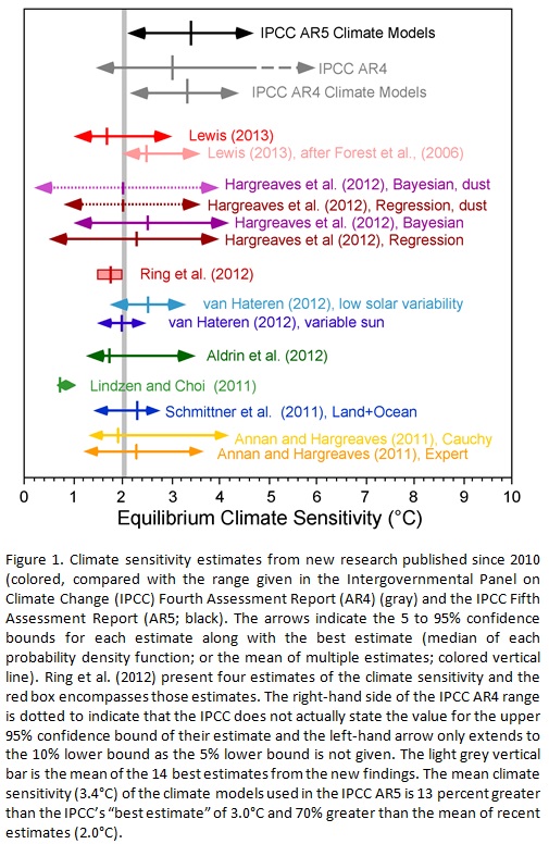
A comparison to various past estimates of ECS is made in figure 5. The base for figure 5 comes from the following weblink :
http://www.cato.org/sites/cato.org/files/wp-content/uploads/gsr_042513_fig1.jpg
See link for the original figure.

Figure 5 : Comparison of the results of this study (1.8) to other recent ECS estimates.
The estimate derived from this study agrees very closely with other recent studies. The gray line on figure 5 at a value of 2.0 represents the mean of 14 recent studies. Looking at the MSE curve in figure 4, 2.0 is essentially flat with 1.8 and would have a similar probability. This study further reinforces the conclusions of other recent studies which suggest climate sensitivity to CO2 is low relative to IPCC estimates .
The big difference with this study is that it is strictly based on the observed data. There are no models involved and only one assumption – that the longer period variation in temperature is driven by CO2 only. Given that the conclusion of a most likely sensitivity of 1.8 ° C / doubling is based on 163 years of observed data, the conclusion is likely to be quite robust.
A brief discussion of the assumption will now be made in light of the conclusion. The question to be asked is : If there are other factors affecting the long period trend of the observed temperature trend (there are many other potential factors, none of which will be discussed in this paper), what does that mean in terms of this best fit ECS curve ?
There are 2 options. If the true ECS is higher than 1.8, by definition , to match the observed data, there has to be some sort of negative forcing in the climate system pushing the temperature down from where it would be expected to be. In this scenario, CO2 forcing would be preventing the temperature trend from falling and is providing a net benefit.
The second option is the true ECS is lower than 1.8. In this scenario, also by definition, there has to be another positive forcing in the climate system pushing the temperature up to match the observed data. In this case CO2 forcing is smaller and poses no concern for detrimental effects.
For both of these options, it is hard to paint a picture where CO2 is going to be significantly detrimental to human welfare. The observed temperature and CO2 data over the last 163 years simply doesn’t allow for it.
Conclusion :
Based on data sets over the last 163 years, a most likely ECS of 1.8 ° C / doubling has been determined. This is a simple calculation based only on data , with no complicated computer models needed.
An ECS value of 1.8 is not consistent with any catastrophic warming estimates but is consistent with skeptical arguments that warming will be mild and non-catastrophic. At the current rate of increase of atmospheric CO2 (about 2.1 ppm/yr), and an ECS of 1.8, we should expect 1.0 ° C of warming by 2100. By comparison, we have experienced 0.86 ° C warming since the start of the HADCRUT4 data set. This warming is similar to what would be expected over the next ~ 100 years and has not been catastrophic by any measure.
For comparison of how unlikely the catastrophic scenario is, the IPCC AR5 estimate of 3.4 has an MSE error nearly as large as assuming that CO2 has zero effect on atmospheric temperature (see fig. 4).
There had been much discussion lately of how the climate models are diverging from the observed record over the last 15 years , due to “the pause”. All sorts of explanations have been posited by those supporting a high ECS value. The most obvious resolution is that the true ECS is lower, such as concluded in this paper. Note how “the pause” brings the observed temperature curve right to the 1.8 ECS synthetic record (see fig. 3). Given an ECS of 1.8, the global temperature is right where one would predict it should be. No convoluted explanations for “the pause” are needed with a lower ECS.
The high sensitivity values used by the IPCC , with their assumption that long term temperature trends are driven by CO2, are completely unsupportable based on the observed data. Along with that, all conclusions of “climate change” catastrophes are also completely unsupportable because they have the high ECS values the IPCC uses built into them (high ECS to get large temperature changes to get catastrophic effects).
Furthermore and most importantly, any policy changes designed to curb “climate change” are also unsupportable based on the data. It is assumed that the need for these policies is because of potential future catastrophic effects of CO2 but that is predicated on the high ECS values of the IPCC.
Files:
I have also attached a spreadsheet with all my raw data and calculations so anyone can easily replicate the work.
ECS Data (xlsx)
=============================================================
About Jeff:
I have followed the climate debate since the 90s. I was an early “skeptic” based on my geologic background – having knowledge of how climate had varied over geologic time, the fact that no one was talking about natural variation and natural cycles was an immediate red flag. The further I dug into the subject, the more I realized there were substantial scientific problems. The paper I am submitting is a paper I have wanted to write for years , as I did the basic calculations several years ago & realized there was no support in the observed data for high climate sensitivity.
All,
Thanks for your comments. Let me say a few words on what I view as the most significant comments.
1) A lot of people have commented about what wasn’t addressed, how the analysis could be done better, etc. I agree with and recognize all of those criticisms. Perhaps I didn’t make my self clear enough at the beginning of the essay that this was a data analysis with a specific assumption – what ECS number would you calculate if you assumed all the longer period trend was from CO2. The reason for doing this isn’t because that is right assumption but because it gives you a base line for comparison.
If you assume all long term change is due to CO2 & you can’t match the observed data with a high ECS value, how can you reasonably expect to have a high sensitivity with other assumptions ? That was fundamentally the point of this essay, which may have been lost in the sauce , so to speak.
The observed data (not some black box climate model) strongly argues against a high ECS – that is the key point I hope everyone takes away
2) Several people commented on TCR vs ECS. Here’s assumption – we are looking at 163 years of data and only looking at the long period of the record (best fit over the entire record, where most of the energy of the signal is located). Yes, CO2 is still being added and yes it may not be a pure ECS but it a lot closer to ECS than TCR.
3) Several people have commented on the choice of HADCRUT4 vs other data sets & data massaging. Just to re-iterate what was said in the body of the essay – all these have negligible effects on this calculation. You might move the ECS value up or down by 0.1 but you certainly won’t move it to a value greater than 3 – a catastrophic value. Llook at the synthetic curves – the data adjustments are small compared to the differences of the observed data and catastrophic trend curves.
4) Comments of lag : definitely recognized but beyond the scope of this analysis. However, unless the lag is decades, this will not substantially alter the calculated event & certainly will not alter the main conclusion – that high ECS is not supported by the observed data
I suppose some may doubt in my comment at 3:13pm that carbon dioxide acts in the same way as moisture in the air in reducing the lapse rate and thus reducing the greater surface warming resulting from the thermal gradient (dry lapse rate) which evolves spontaneously simply because it is the state of greatest entropy that can be accessed in the gravitational field.
Many think, as climatologists teach their climatology students, that the release of latent heat is what reduces the lapse rate over the whole troposphere.
Well it’s not the primary cause of any overall effect on the lapse rate. That effect is fairly homogeneous, so the mean annual lapse rate in the tropics, for example is fairly similar at most altitudes. But the release of latent heat during condensation is not equal at all altitudes and warming at all altitudes would not necessarily reduce the gradient anyway. In fact, one would expect more such warming in the lower troposphere.
The effect of reducing the lapse rate is to cool temperatures in the lower 4 or 5Km of the troposphere and raise them in the upper troposphere, so that this all helps to retain radiative balance with the Sun, such as is observed.
So where is all the condensation in the uppermost regions of the troposphere and why is there apparently a cooling effect from whatever latent heat is released in the lower altitudes below 4 or 5Km?
It’s nonsense what climatologists teach themselves, and the claims made are simply not backed up by physics.
Radiation can transfer energy from warmer to cooler molecules within the system being considered, so this transfers energy far faster than the slow process that involves molecular collisions. That is why the gradient is reduced and the reduction also happens on other planets where no water is present. That is why water molecules and suspended droplets in the atmosphere, as well as carbon dioxide and other GHG all lead to cooler surface temperatures.
@Robert of Texas says:
February 13, 2014 at 4:04 pm
The problem, Robert, is that you have it exactly the wrong way round. If Jeff L shows a correlation against a transient sensitivity which is X then the equilibrium sensitivity is greater than X. Hence, if Jeff L’s analysis were valid then it would prove a higher equibrium sensitivity than his result. In other words it would be a lower bound. The reality is that his analysis method is flawed.
Jeff L. says:
February 13, 2014 at 4:49 pm
“Perhaps I didn’t make my self clear enough at the beginning of the essay that this was a data analysis with a specific assumption – what ECS number would you calculate if you assumed all the longer period trend was from CO2.”
and there is no significant input from natural variability over that time period either.
I think the work you have done is valuable in that it describes what must be true if all the other parts of the equation are set to zero. Any changes to those values would then have to be applied to the figure so derived. Some might be up, some down. The chance that they would all cancel out nicely or all be in the same direction are small.
The “”CLIMATE SENSITIVITY” was elaborated in a model of Schneider&Maas, 1975.
This model was proven wrong in its physics, has no merit….therefore, all this curve
matching and best guess fiting is without any sense. There is unrefuted literature
out, proving the failure of Schneider and Maas. We better do something what generates
progress instead of remasticating the old sensitivity weed….
Jeff L.
I suspect that we cross-posted, but just to reiterate: you have not put an upper bound on ECS. If your analysis were valid, (which it isn’t), then you have put a lower bound on the ECS.
The reality is that if you match HADCRUT4 against the forcing (RCP suite) and OHC data (Levitus) using a transient model, then you will find that your equilibrium sensitivity should come out around 1.6 deg C/Watt/m2 assuming linearity of net flux response to temperature. What you are doing is retrogressive relative to that result – which is quite well published.
Paul_K says:
February 13, 2014 at 5:15 pm
Remind me once again about how the models so well predicted things with regard to forcings that this is what has actually occurred.
http://i29.photobucket.com/albums/c274/richardlinsleyhood/HansenUpdated_zpsb8693b6e.png
Just what WERE the model forcing settings and their combined outcomes for Scenario C again?
We seem to be tiptoeing down that dotted line after all, models or not.
Dr Burns says:
February 13, 2014 at 2:53 pm
Since your chart has no provenance or underlying data, it’s useless.
It appears to be a chart of CO2 vs ice age from the Siple core. However, it is well known that the snow doesn’t close up the bubbles until the firn is squashed down by subsequent winters. As a result, the air enclosed in the bubble is ALWAYS younger than the age of the ice itself.
There is both a graph and the underlying Siple data here … and Dr. Burns, please don’t bother posting further uncited, un-commented graphs with no provenance. They are merely advertising and anecdote, and are a distraction from actual science.
Regards,
w.
A fine assessmet, based on the assumptions given.
Take the IPCC assumption,their temperature reconstruction and CO2 concentrations estimates and analyse thus.The accused magic gas is found innocent?.
Or insufficient evidence?
Based on the geological record, climate sensitivity to all kinds of effects is tiny.
A bistable system seems evident, with 1000s of years between the mystery trigger that oscillates between ice age or not ice age.
The catastrophic warm event, much feared by the team, is not evident.
Greig says:
February 13, 2014 at 3:02 pm
The problem with this analysis is that it assumes that all warming is caused by CO2, which is obviously wrong when viewing the HADCRUT plot. There is clearly a natural components which caused warming in early 1900s, and some cooling 1940-1970. It is faulty logic to make an assumption that is wrong, and then declaring that if there is a natural component then the situation is even better. In fact, addition of a natural component that suggests a higher ECS, is not a good thing because we don’t know what are the future natural drivers to the climate. There may be in the future natural warming added to CO2 forcing.
______
You’re not exactly catching the strategy that Jeff L. is employing. The idea is to grant the warmists their apparent assumption that CO2 is the driver of temperature change, and see, using actual observations, what climate sensitivity this would imply. The answer, given Jeff’s methods, is that sensitivity would be considerably lower than what would be needed to cause alarm. Jeff is not necessarily assuming that the warmists’ idea is correct. As he states clearly:
“The rest of this paper will explore testing the hypothesis of high ECS based on the observed data. I want to re-iterate the assumption of this hypothesis, which is also the assumption of the catastrophists position, that all longer term temperature change is driven by changes in CO2. I do not want to imply that I necessarily endorse this assumption, but I do want to illustrate the implications of this assumption.”
He takes their assumption at face value and shows how it explodes when applied to real historical data.
You’re not exactly catching the strategy that Jeff L. is employing.
On the contrary, I fully understand the strategy, merely pointing out that it achieves nothing of value. HADCRUT clearly shows natural warming and cooling, and Jeff L is fitting a curve based on a calculation that does not contain the same natural warming/cooling effects. Hence the number for ECS is wrong, and it may be any number between 1 and 5 depending on how the Earth’s temperature would have changed in the absence of a change in CO2. The only way to reach a number for ECS is to know exactly what the natural warming/cooling is. And we don’t know that. Therefore this analysis does not reveal anything valid on future warming.
Further, as others have noted, the lag in warming (eg due to ocean buffering, feedbacks from albedo, etc) is also not included in the analysis, and this is also critical to understanding future warming.
I am also no fan of the climate models being used in policy making, and well aware that they are not matching observations as acknowledged by the IPCC.
The fact is we do not know how much (or even if) it will warm in the future, and we should acknowledge that and policy should match.
Willis Eschenbach says:
February 13, 2014 at 5:21 pm
“There is both a graph and the underlying Siple data here …”
Adding that to the temperature record fits pretty well after 1900 or so but before……
http://i29.photobucket.com/albums/c274/richardlinsleyhood/200YearsofTemperatureSatelliteThermometerandProxySimple_zpsf4c9b7bf.gif
[ snip – fake email address used to submit comments, policy violation
MX record about ‘gmail.edu’ does not exist.
trafamadore@gmail.edu – Result: Bad – mod]
But who relies on Hansen? Anyone?
If Hansen is involved, or someone trained by Hansen, or someone who co authored with Hansen, or is associated with major universities that use data prepared by his NASA organization I use the verify before accepting any results.
If you sleep with scum like Hansen, you will get his fleas.
@Paul_K-Key words “RCP suite”-whether this accurately reflects the actual forcings acting on the system is another matter entirely.
Or whether explaining as much of the variance as possible really amounts to getting the correct sensitivity value.
RichardLH says:
February 13, 2014 at 5:20 pm
I am not talking about GCM predictions. Your comment is irrelevant. Observation-based estimates of climate sensitivity are normally based on transient behaviour, typically captured in a simple zero-dimensional flux balance equation. This is a differential equation which requires forward modeling, not a memoryless equation, such as that used by Jeff L.
Paul_K says:
February 13, 2014 at 5:54 pm
“I am not talking about GCM predictions. Your comment is irrelevant. Observation-based estimates of climate sensitivity are normally based on transient behaviour, typically captured in a simple zero-dimensional flux balance equation.”
Climate sensitivity calculations (transient or otherwise) are what the models base their outputs on.
Observation-based estimates of climate sensitivity are normally based on transient behaviour, typically captured in a simple zero-dimensional flux balance equation should at least have some bearing or relevance on the root of those calculations.
If the models using those same calculations don’t track reality at all, how then can we rely on the calculations themselves?
@timetochooseagain says:
February 13, 2014 at 5:48 pm
I don’t doubt that the RCP suite is inaccurate. My main point is that if you consider this mainstream data, it takes you to a different lower conclusion about ECS than Jeff L’s..
@RichardLH says:
February 13, 2014 at 6:01 pm
Boy, are you confused or what? The GCMs calculate climate sensitivity based on their long-term predictions of temperature for a given input forcing scenario. Are they wrong? Yes, without a doubt.
Does this have anything to do with observation-based estimates? Well it would if the GCMs could match historical estimates of net flux, ocean heat uptake, forcings and tropospheric temperatures.
Can they do that? No.
So GCM predictions have nothing to do with the application of offline aggregate net flux balance calculations,
Paul_K says:
February 13, 2014 at 6:17 pm
“So GCM predictions have nothing to do with the application of offline aggregate net flux balance calculations”
But the net flux balance calculations are part of what the model is supposed to observe. If that figure is wrong (or there is in fact no net imbalance) then where are we?
Assuming that the amount of heat CO2 can absorb is finite (I’m not a scientist, but recall reading that it is), doesn’t that have to be considered as part of the formula? At some point the temperature rise would begin to flatten with CO2 increasing.
@Paul_K
Yes, agreement! I seem to find few people I agree with these days.
@RichardLH says:
February 13, 2014 at 6:29 pm
We don’t know what the net flux imbalance is, that’s for sure. Satellite measurements have high precision but low accuracy. We do know that it has been declining since the turn of the century – from direct satellite measurement, from (derivative of) ocean heat content data and from (the derivative of) MSL data. There may still be a positive flux imbalance and all of the extra energy is going into ocean heat, but the more interesting question is why is the net TOA downward flux declining in light of the increasing forcing from CO2.? I think I know the answer to this question but I am waiting for an offer from a rich fossil fuel company to produce it..
Jeff L,
Just one more time…
You use an equation that states
Expected change in (surface) temperature = Forcing as a ratio to a doubling of CO2 times the equilibrium (surface) temperature as a result of a doubling of CO2.
The LHS of this equation is clearly an equilibrium response. Now in any circumstance the equilibrium response is expected to be greater than the transient response. Yes? But you substitute the realworld transient response for the LHS of this equation in order to estimate the equlibrium response to a doubling of CO2 from the RHS of this equation, the ECS. Hence you end up with a lower bound on the estimate of ECS, by your methodology. Is it right? No.
@ur momisugly Willis re cpi- I am not clever enough to understand the maths so I humbly ask isn’t the point that if we assume CPI is related to surface temperature we can work out the magnitude of the imaginary relationship?
As you point out we can look at this for changes in CPI, CO2, divorce rates, number of domestic guinea pigs etc.
The curve fit doesn’t imply causation or even correlation but when we assume causation it can give an idea of the magnitude of the hypothetical effect can’t it? Using Jeff’s technique we could for example look at what doubling divorce rates would do to global temperature assuming they were related. This would be nonsense but while over simple it might not be nonsense for CO2 . it is certainly interesting because it is based on the generous assumption that all observed warming in hadcrut 4 was co2 related.
Willis,
Some push pack. Dividing data into three 50 year periods will mainly show us that the longer (and shorter) than 50 year ocean oscillations do not cancel out in that short a period. (and probably not 150 years either, I admit).
Also, you don’t need all the other forcings which you admit are unknown. You don’t need any of them. You assume that CO2 is the entire forcing. You end up with a climate sensitivity of 1.8 (thanks for showing the calculations Jeff L.) which is higher than the actual climate sensitivity if there are other positive forcings. Only if there are net negative non-GHC forcings, would the climate sensitivity be higher. Based on “persistence forecasting” we can have some confidence (its “likely”) that the positive unknown forcings of the past several hundred years are continuing. Therefore, it is also “likely” that climate sensitivity is less than 1.8. This is a very simple semi-empirical model that I’ve used to explain climate sensitivity many times. With all the problems I’m sure we can find with it, I’ll bet you that it shows more skill than the IPCC and Hansen super computer model projections over the next 86 years. How about a bet on on the relative skills of the IPCC mean sensitivity 3 (you) versus the 1.8 of this model (me) for the remainder of this century. Mosh and Anthony can work out the details and be the judges. What do you want to bet. I’m so confident, I’m willing to bet everything I own in 2100. Even though you may correctly argue that there is no real climate sensitivity, we’ll have a calculated one based on CO2 emissions and temp in 86 years. Exciting, yes, and good deal for you. Actually Mosh might also want to bet and take Hansen’s high end of the lukewarmer sensitivity continuum which would be, ah what? And Anthony could take Lindzen’s climate sensitivity of 1, but then we’ve have no judges, ah ,no confirmation biasless judges.
Only time to read the first half of comments so maybe someone already beat me out and devised some fantastic bets- or maybe we have to go to The Blackboard to see if that’s true.
Cautious Doug