This exercise in data analysis pins down a value of 1.8C for ECS.
Guest essay by Jeff L.
Introduction:
If the global climate debate between skeptics and alarmists were cooked down to one topic, it would be Equilibrium Climate Sensitivity to CO2 (ECS) , or how much will the atmosphere warm for a given increase in CO2 .
Temperature change as a function of CO2 concentration is a logarithmic function, so ECS is commonly expressed as X ° C per doubling of CO2. Estimates vary widely , from less than 1 ° C/ doubling to over 5 ° C / doubling. Alarmists would suggest sensitivity is on the high end and that catastrophic effects are inevitable. Skeptics would say sensitivity is on the low end and any changes will be non-catastrophic and easily adapted to.
All potential “catastrophic” consequences are based on one key assumption : High ECS ( generally > 3.0 ° C/ doubling of CO2). Without high sensitivity , there will not be large temperature changes and there will not be catastrophic consequences. As such, this is essentially the crux of the argument : if sensitivity is not high, all the “catastrophic” and destructive effects hypothesized will not happen. One could argue this makes ECS the most fundamental quantity to be understood.
In general, those who are supportive of the catastrophic hypothesis reach their conclusion based on global climate model output. As has been observed by many interested in the climate debate, over the last 15 + years, there has been a “pause” in global warming, illustrating that there are significant uncertainties in the validity of global climate models and the ECS associated with them.
There is a better alternative to using models to test the hypothesis of high ECS. We have temperature and CO2 data from pre-industrial times to present day. According to the catastrophic theory, the driver of all longer trends in modern temperature changes is CO2. As such, the catastrophic hypothesis is easily tested with the available data. We can use the CO2 record to calculate a series of synthetic temperature records using different assumed sensitivities and see what sensitivity best matches the observed temperature record.
The rest of this paper will explore testing the hypothesis of high ECS based on the observed data. I want to re-iterate the assumption of this hypothesis, which is also the assumption of the catastrophists position, that all longer term temperature change is driven by changes in CO2. I do not want to imply that I necessarily endorse this assumption, but I do want to illustrate the implications of this assumption. This is important to keep in mind as I will attribute all longer term temperature changes to CO2 in this analysis. I will comment at the end of this paper on the implications if this assumption is violated.
Data:
There are several potential datasets that could be used for the global temperature record. One of the longer and more commonly referenced datasets is HADCRUT4, which I have used for this study (plotted in fig. 1) The data may be found at the following weblink :
http://www.cru.uea.ac.uk/cru/data/temperature/HadCRUT4-gl.dat
I have used the annualized Global Average Annual Temperature anomaly from this data set. This data record starts in 1850 and goes to present, so we have 163 years of data. For the purposes on this analysis, the various adjustments that have been made to the data over the years will make very little difference to the best fit ECS. I will calculate what ECS best fits this temperature record, given the CO2 record.

Figure 1 : HADCRUT4 Global Average Annual Temperature Anomaly
The CO2 data set is from 2 sources. From 1959 to present, the Mauna Loa annual mean CO2 concentration is used. The data may be found at the following weblink :
ftp://aftp.cmdl.noaa.gov/products/trends/co2/co2_annmean_mlo.txt
For pre-1959, ice core data from Law Dome is used. The data may be found at the following weblink :
ftp://ftp.ncdc.noaa.gov/pub/data/paleo/icecore/antarctica/law/law_co2.txt
The Law Dome data record runs from 1832 to 1978. This is important for 2 reasons. First, and most importantly, it overlaps Mauna Loa data set. It can easily be seen in figure 2 that it is internally consistent with the Mauna Loa data set, thus providing higher confidence in the pre-Mauna Loa portion of the record. Second, the start of the data record pre-dates the start of the HADCRUT4 temperature record, allowing estimates of ECS to be tested against the entire HADCRUT4 temperature record. For the calculations that follow, a simple splice of the pre-1959 Law Dome data onto the Mauna Loa data was made , as the two data sets tie with little offset.

Figure 2 : Modern CO2 concentration record from Mauna Loa and Law Dome Ice Core.
Calculations:
From the above CO2 record, a set of synthetic temperature records can be constructed with various assumed ECS values. The synthetic records can then be compared to the observed data (HADCRUT4) and a determination of the best fit ECS can be made.
The equation needed for the calculation of the synthetic temperature record is as follows :
∆T = ECS* ln(C2/C1)) / ln(2)
where :
∆T = Change in temperature, ° C
ECS = Equilibrium Climate Sensitivity , ° C /doubling
C1 = CO2 concentration (PPM) at time 1
C2 = CO2 concentration (PPM) at time 2
For the purposes of this test of sensitivity, I set time 1 to 1850, the start of the HADCRUT4 temperature dataset. C1 at the same time from the Law Dome data set is 284.7 PPM. For each year from 1850 to 2013, I use the appropriate C2 value for that time and calculate ∆T with the formula above. To tie back to the HADCRUT4 data set, I use the HADCRUT4 temperature anomaly in 1850 ( -0.374 ° C) and add on the calculated ∆T value to create a synthetic temperature record.
ECS values ranging from 0.0 to 5.0 ° C /doubling were used to create a series of synthetic temperature records. Figure 3 shows the calculated synthetic records, labeled by their input ECS, as well as the observed HADCRUT4 data.

Figure 3: HADCRUT4 Observed data and synthetic temperature records for ECS values between 0.0 and 5.0 ° C / doubling. Where not labeled, synthetic records are at increments of 0.2 ° C / doubling. Warmer colors are warmer synthetic records.
From Figure 3, it is visually apparent that a ECS value somewhere close to 2.0 ° C/ doubling is a reasonable match to the observed data. This can be more specifically quantified by calculating the Mean Squared Error (MSE) of the synthetic records against the observed data. This is a “goodness of fit” measurement, with the minimum MSE representing the best fit ECS value. Figure 4 is a plot of MSE values for each ECS synthetic record.

Figure 4 : Mean Squared Error vs ECS values. A few ECS values of interest are labeled for further discussion
In plotting, the MSE values, a ECS value 1.8 ° C/ doubling is found to have the minimum MSE and thus is determined to be the best estimate of ECS based on the observed data over the last 163 years.
Discussion :
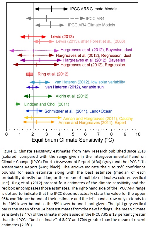
A comparison to various past estimates of ECS is made in figure 5. The base for figure 5 comes from the following weblink :
http://www.cato.org/sites/cato.org/files/wp-content/uploads/gsr_042513_fig1.jpg
See link for the original figure.

Figure 5 : Comparison of the results of this study (1.8) to other recent ECS estimates.
The estimate derived from this study agrees very closely with other recent studies. The gray line on figure 5 at a value of 2.0 represents the mean of 14 recent studies. Looking at the MSE curve in figure 4, 2.0 is essentially flat with 1.8 and would have a similar probability. This study further reinforces the conclusions of other recent studies which suggest climate sensitivity to CO2 is low relative to IPCC estimates .
The big difference with this study is that it is strictly based on the observed data. There are no models involved and only one assumption – that the longer period variation in temperature is driven by CO2 only. Given that the conclusion of a most likely sensitivity of 1.8 ° C / doubling is based on 163 years of observed data, the conclusion is likely to be quite robust.
A brief discussion of the assumption will now be made in light of the conclusion. The question to be asked is : If there are other factors affecting the long period trend of the observed temperature trend (there are many other potential factors, none of which will be discussed in this paper), what does that mean in terms of this best fit ECS curve ?
There are 2 options. If the true ECS is higher than 1.8, by definition , to match the observed data, there has to be some sort of negative forcing in the climate system pushing the temperature down from where it would be expected to be. In this scenario, CO2 forcing would be preventing the temperature trend from falling and is providing a net benefit.
The second option is the true ECS is lower than 1.8. In this scenario, also by definition, there has to be another positive forcing in the climate system pushing the temperature up to match the observed data. In this case CO2 forcing is smaller and poses no concern for detrimental effects.
For both of these options, it is hard to paint a picture where CO2 is going to be significantly detrimental to human welfare. The observed temperature and CO2 data over the last 163 years simply doesn’t allow for it.
Conclusion :
Based on data sets over the last 163 years, a most likely ECS of 1.8 ° C / doubling has been determined. This is a simple calculation based only on data , with no complicated computer models needed.
An ECS value of 1.8 is not consistent with any catastrophic warming estimates but is consistent with skeptical arguments that warming will be mild and non-catastrophic. At the current rate of increase of atmospheric CO2 (about 2.1 ppm/yr), and an ECS of 1.8, we should expect 1.0 ° C of warming by 2100. By comparison, we have experienced 0.86 ° C warming since the start of the HADCRUT4 data set. This warming is similar to what would be expected over the next ~ 100 years and has not been catastrophic by any measure.
For comparison of how unlikely the catastrophic scenario is, the IPCC AR5 estimate of 3.4 has an MSE error nearly as large as assuming that CO2 has zero effect on atmospheric temperature (see fig. 4).
There had been much discussion lately of how the climate models are diverging from the observed record over the last 15 years , due to “the pause”. All sorts of explanations have been posited by those supporting a high ECS value. The most obvious resolution is that the true ECS is lower, such as concluded in this paper. Note how “the pause” brings the observed temperature curve right to the 1.8 ECS synthetic record (see fig. 3). Given an ECS of 1.8, the global temperature is right where one would predict it should be. No convoluted explanations for “the pause” are needed with a lower ECS.
The high sensitivity values used by the IPCC , with their assumption that long term temperature trends are driven by CO2, are completely unsupportable based on the observed data. Along with that, all conclusions of “climate change” catastrophes are also completely unsupportable because they have the high ECS values the IPCC uses built into them (high ECS to get large temperature changes to get catastrophic effects).
Furthermore and most importantly, any policy changes designed to curb “climate change” are also unsupportable based on the data. It is assumed that the need for these policies is because of potential future catastrophic effects of CO2 but that is predicated on the high ECS values of the IPCC.
Files:
I have also attached a spreadsheet with all my raw data and calculations so anyone can easily replicate the work.
ECS Data (xlsx)
=============================================================
About Jeff:
I have followed the climate debate since the 90s. I was an early “skeptic” based on my geologic background – having knowledge of how climate had varied over geologic time, the fact that no one was talking about natural variation and natural cycles was an immediate red flag. The further I dug into the subject, the more I realized there were substantial scientific problems. The paper I am submitting is a paper I have wanted to write for years , as I did the basic calculations several years ago & realized there was no support in the observed data for high climate sensitivity.
Here you go, it’s the secret of climate that we’ve searched for so long …

SO … I can use that to calculate the climate sensitivity of the relationship. Just like the head post, I’ve used the log of the underlying data (to base 2, as in the head post).
Only problem?
The red line is not CO2. It’s the CPI, the Consumer Price Index, since 1850 …
Jeff, I hope you can see that this type of “match up the curves” is not all that diagnostic …
w.
PS: If you truly want to do this kind of analysis, you need to use a lagging equation on your forcings, and you need to include all known forcings. The problem is, most forcings we have no clue about for the 1800’s … so we end up with error bars (which you’ve neglected) from floor to ceiling.
Jeff, what is your uncertainty estimate, plus/minus degrees C ?
Also what you are estimating is the transient climate response since it will take additional time for the oceans to adjust to changes in temperature.
Continuing from my comment at 2:16pm, the inevitable conclusion is that it is not greenhouse gases that are raising the surface temperature by 33 degrees or whatever, but the fact that the thermal profile is already established by the force of gravity acting at the molecular level on all solids, liquids and gases. So the “lapse rate” is already there, and indeed we see it in the atmospheres of other planets as well, even where no significant solar radiation penetrates.
In fact, because the “dry” lapse rate is steeper, and that is what would evolve spontaneously in a pure nitrogen and oxygen atmosphere, and because we know that the wet adiabatic lapse rate is less steep than the dry one, it is obvious that the surface temperature is not as high because of these greenhouse gases. Carbon dioxide (being one molecule in about 2,500 other molecules) has very little effect, but whatever effect it does have would thus be very minor cooling.
I don’t care what you think you can deduce from whatever apparent correlation you think you can demonstrate from historical data, there is no valid physics which points to carbon dioxide warming.
You are looking at transient climate response (TCR), not equilibrium climate sensitivity (ECS). The IPCC AR4 TCR numbers are 1.5 to 2.8 C per doubling of CO2, with a mean estimate of 2.1. In the AR5, the average TCR across CMIP5 models was 1.8 C per doubling. So technically your result ends up being exactly the same as the models :-p
Mosher says
“‘In general, those who are supportive of the catastrophic hypothesis reach their conclusion based on global climate model output.”
Wrong. Hansen for example relies on Paleo data.”
Really Mosh? No one has ever shown any DATA that demonstrates that CAGW is real. That is the problem, if there was DATA that demonstrates that, there would be no issue whatsover. with us skeptics, except for perhaps on how to address/solve it. CAGW currently exists ONLY in the models. Hansen does not rely on Paleo data to prove CAGW. Perhaps he uses paleo data, sticks it into his MODEL, and viola!…. CAGW.
Aslo, if you are mentioning Paleo data because of the recent paper. I scanned through the paper and saw no graphical presentation of any of the temperature data the were fitting the models too. Is that because all of the paleo temperature data series being investigated were “hockey sticks” and they are trying to “Hide” that fact as best they can?
Granting the analysis, the result is that 1.8 C is the upper limit of climate sensitivity, not the most likely value. The reason is that the analysis assumes that all the warming since 1850 is due to CO2. Enter any other source of warming, the fraction of warming due to CO2 decreases below 1.0, and climate sensitivity is less than 1.8 C.
It’s not the equilibrium climate sensitivity you’re working here with, by the way, but the transient climate sensitivity. Equilibrium climate sensitivity is determined by the final temperature state reached after the GHG emissions stop and atmospheric [CO2] has become constant (no longer increasing). Transient CS is the immediate increase in air temperature in response to steadily increasing CO2.
That all said, there is still zero evidence that any of the warming since 1880 is due to increased atmospheric CO2.
“The problem with this analysis is that it assumes that all warming is caused by CO2, which is obviously wrong when viewing the HADCRUT plot.”
its also wrong given what we know about other GHG forcings.
all that said, he almost has all of the pieces.. many others have done similar efforts.
they are used by the IPCC.
There are 3 sources of estimates
A) Paleo estimates ( LGM typically)
B) observation estimates ( like this one and Nic Lewis)
C) models.
Note. Most folks put higher weights on A and B. Hansen for example argues that C) is the least
reliable.
This effort falls in the B) class.
Its a start, but the author would do well to read all the papers that have done similar estimates.
once upon a time Nic Lewis did this. Rather than working from ignorance he read the science.
He found some areas that needed improvement. He improved known approaches. He came up
with lowered estimates. he testified in from of parliment.
Here is a lesson. If you want to argue that sensitivity as a metric makes no sense or makes unwarranted assumptions.. nobody is going to listen to you. Thats voice in the wilderness stuff. You are outside the tent pissing in.
IF you read the science, find assumptions, mistakes, etc and come up with improvements,
then you can make a difference.
Your choice: stay on the outside and make no difference. work from the inside and improve.
simple choice, you are free to do either.
@Zeke Hausfather-No, he’s not looking at that either. He’s not looking at anything. There are a number of reasons this isn’t even an estimate of the “transient response”
But as usual the “let’s push the number higher” crowd wants people to only listen to their arguments that whenever anyone gets an answer they don’t like, that the truth can only be higher. it’s got to be higher. Because the real answer is ~3 and you just known.
Guess what. You’re wrong. Really badly wrong.
I got 1.71 using a similar approach.
http://judithcurry.com/2013/05/16/docmartyns-estimate-of-climate-sensitivity-and-forecast-of-future-global-temperatures/
I actually think that this methodology is rather good at resolving the lag between transient and ‘equilibrium’ climate sensitivity. The inflection around the 50’s in the Keeling Curve should be reflected in the line shape of temperature; which it does if you assume no lag. You can play with any lag you like, but warming and pause, screw up any lag >12 months.
Haven’t read it all the way through yet, but the analysis seems to be assuming that all of the warming in recent decades is the result of CO2.
Jeff: Do not despair. There are wriggles in the data (mustn’t call then cycles) that cannot be CO2 related so we need to take that into account as well.
http://i29.photobucket.com/albums/c274/richardlinsleyhood/Fig8HadCrutGISSRSSandUAHGlobalAnnualAnomalies-Aligned1979-2013withGaussianlowpassandSavitzky-Golay15yearfilters_zps670ad950.png
And the future (LOWESS style) looks downwards!
MarkW says:
February 13, 2014 at 3:30 pm
“Haven’t read it all the way through yet, but the analysis seems to be assuming that all of the warming in recent decades is the result of CO2.”
You’re not suggesting that we need to flatten the CO2 line still further because there might be some natural variability in there as well are you? You know, like what the IPCC says there is?
Zeke Hausfather says:
February 13, 2014 at 3:14 pm
“You are looking at transient climate response (TCR), not equilibrium climate sensitivity (ECS). The IPCC AR4 TCR numbers are 1.5 to 2.8 C per doubling of CO2, with a mean estimate of 2.1”
Remind me again why we are tiptoeing down the dotted line drawn by Scenario C?
http://i29.photobucket.com/albums/c274/richardlinsleyhood/HansenUpdated_zpsb8693b6e.png
Pat Frank says:
February 13, 2014 at 3:16 pm
“That all said, there is still zero [hard] evidence that any of the warming since 1880 is due to increased atmospheric CO2.”
+1
Let me support what Pat Frank writes You write ” I want to re-iterate the assumption of this hypothesis, which is also the assumption of the catastrophists position, that all longer term temperature change is driven by changes in CO2.”
There is nothing wrong with this as long as you state, explicitly, that what you are estimating is the maximum value for climate sensitivity. If all of the observed rise in temperature is due to natural causes, and not CO2, then the value of climate sensitivity is 0 C
Jim Cripwell says:
February 13, 2014 at 4:00 pm
“There is nothing wrong with this as long as you state, explicitly, that what you are estimating is the maximum value for climate sensitivity. If all of the observed rise in temperature is due to natural causes, and not CO2, then the value of climate sensitivity is 0 C”
But that’s heresy! CO2 MUST be the cause. I mean…….
“Steven Mosher
its also wrong given what we know about other GHG forcings.
all that said, he almost has all of the pieces.. many others have done similar efforts.
they are used by the IPCC.
There are 3 sources of estimates
A) Paleo estimates ( LGM typically)”
I am quite happy for them to use the ice core CO2/Temperature record to calculate ECS, as long as they use the atmospheric Dust levels as a proxy for aerosol forcing. Given that dust levels change by three orders of magnitude from warm to cold ages, with 1000 times more atmospheric dust in the ice ages when compared to the warmest parts of the record, they don’t use them
Any reconstruction that ignores the dust levels is completely and utterly bogus; but then you knew that Mosher.
Seems to me the point is to put an upper limit on sensitivity – not that the value is likely. If the upper limit (using ridiculous assumptions all in favor of CAGW) is less than 2C, then the models are falsified (again).
So if the point was to actually compute the sensitivity, the approach is too simple and inaccurate and would have to identify and categorize all of the forcings If the point was merely to show 2C+ sensitivity is not supported by data, the approach seems to work (at least for me).
I do like the simple approach. I do also understand it isn’t the same as computing the sensitivity; Its a way of putting a boundary on it.
Mosher says “Hansen for example relies on Paleo data.”
Let’s take the last glacial maximum and Hansen’s estimates based on that (and he actually wrote a paper on it). Temps were -5.0C lower, CO2 was at 185 ppm. Hansen should have calculated climate sensitivity of 8.3C per doubling based on those numbers. But he came up with 3.0C per doubling. How did he manage that? Only two possible explanations. He is very bad at the math of global warming or he faked up the numbers.
Steven Mosher:
“Hansen for example relies on Paleo data.”
And he was SO right about how all this would play out wasn’t he?
http://i29.photobucket.com/albums/c274/richardlinsleyhood/HansenUpdated_zpsb8693b6e.png
What was Scenario C again? Why would we follow that dotted line?
Here’s one
http://i56.tinypic.com/f3tlb6.jpg
I did a few years back.
You can also compare CO2 to major league home runs and get a nice fit.
And I’ve done the CO2 to HADCRUT4 comparison, goes something like this:
1850 – 1878 CO2 up less than 1 ppm temp up 0.4 deg 28 yrs
1878 – 1911 CO2 up 5 ppm temp down a minus -0.4 deg 33 yrs
1911 – 1944 CO2 up 15 ppm temp up 0.7 deg 33 yrs
1944 – 1977 CO2 up 30 ppm temp down minus -0.4 deg 33yrs
1977 – 2010 CO2 up 60 ppm temp up 0.8 ppm 33 yrs
Looks like CO2 doesn’t have much to do with it and some sort of 66 year cycle seems to have a lot more.
Personally think the feedbacks are negative, and climate sensitivity is less than 1.2 deg Celsius per doubling of CO2.
Thank you for your research and publication.
I feel that if the HADCRUT, and other temperature records, including the satellite data, have been so grossly adjusted to reduce warming periods before CO2 started its rapid increase and to increase warming as the atmospheric CO2 levels increased, that they are false. This dishonest and criminal tampering with the data to suggest global warming that just never happened means that accurate and true measured temperature to compute global temperature simply do not exist.
Thus, we have no measured data to compare with modeling results. Unless something like another little ice age (which I hope does not occur) cools to the extent that future data cannot be adjusted upward without it being obviously and criminally altered, then we are stuck with adjusted data.
The solution to the problem seems to be to elect politicians who will disavow global warming, un-fund those who claim it is real (as happened in Australia, at least at the federal level). and refocus our research to real problems. If we did not fund any any more dishonest “global warming, climate change, …, scientists”, that might partially solve the problem.
Engineers must often seek professional registration before they engineer projects, and the registered engineers are accountable for their work. MDs are also held accountable for their work via malpractice lawsuits, fines, etc. and they too must be certified as professionals. Perhaps it is time to make scientists and lawyers accountable for the honesty and quality of their work.
Steve Case says:
February 13, 2014 at 4:25 pm
“Looks like CO2 doesn’t have much to do with it and some sort of 66 year cycle seems to have a lot more.”
The data says you’re right.
http://i29.photobucket.com/albums/c274/richardlinsleyhood/Fig8HadCrutGISSRSSandUAHGlobalAnnualAnomalies-Aligned1979-2013withGaussianlowpassandSavitzky-Golay15yearfilters_zps670ad950.png
Alex Hamilton says: February 13, 2014 at 3:13 pm
In fact, because the “dry” lapse rate is steeper, and that is what would evolve spontaneously in a pure nitrogen and oxygen atmosphere, and because we know that the wet adiabatic lapse rate [with water vapor] is less steep than the dry one, it is obvious that the surface temperature is not as high because of these greenhouse gases. Carbon dioxide (being one molecule in about 2,500 other molecules) has very little effect, but whatever effect it does have would thus be very minor cooling.
Absolutely, great comment.
If only Mosher et al would read & understand Dr. Hans Jelbring’s paper
http://ruby.fgcu.edu/courses/twimberley/EnviroPhilo/FunctionOfMass.pdf
Jeff L,
Please don’t take my comments as too negative, because I think it is always good for people to test stuff for themselves, and I am honestly not trying to discourage you, but…
That said, your analysis is flawed in a number of different ways. (1) You cannot fit a memoryless formula, which relates equilibrium temperature change to forcing, to realworld data which should reflect transient temperature change against forcing (2) you are assuming that all of the temperature change is due to CO2 (3) you are ignoring the spurious nature of your final correlation/prediction which should be evident to you if you examine the cyclic nature of your error function.