This exercise in data analysis pins down a value of 1.8C for ECS.
Guest essay by Jeff L.
Introduction:
If the global climate debate between skeptics and alarmists were cooked down to one topic, it would be Equilibrium Climate Sensitivity to CO2 (ECS) , or how much will the atmosphere warm for a given increase in CO2 .
Temperature change as a function of CO2 concentration is a logarithmic function, so ECS is commonly expressed as X ° C per doubling of CO2. Estimates vary widely , from less than 1 ° C/ doubling to over 5 ° C / doubling. Alarmists would suggest sensitivity is on the high end and that catastrophic effects are inevitable. Skeptics would say sensitivity is on the low end and any changes will be non-catastrophic and easily adapted to.
All potential “catastrophic” consequences are based on one key assumption : High ECS ( generally > 3.0 ° C/ doubling of CO2). Without high sensitivity , there will not be large temperature changes and there will not be catastrophic consequences. As such, this is essentially the crux of the argument : if sensitivity is not high, all the “catastrophic” and destructive effects hypothesized will not happen. One could argue this makes ECS the most fundamental quantity to be understood.
In general, those who are supportive of the catastrophic hypothesis reach their conclusion based on global climate model output. As has been observed by many interested in the climate debate, over the last 15 + years, there has been a “pause” in global warming, illustrating that there are significant uncertainties in the validity of global climate models and the ECS associated with them.
There is a better alternative to using models to test the hypothesis of high ECS. We have temperature and CO2 data from pre-industrial times to present day. According to the catastrophic theory, the driver of all longer trends in modern temperature changes is CO2. As such, the catastrophic hypothesis is easily tested with the available data. We can use the CO2 record to calculate a series of synthetic temperature records using different assumed sensitivities and see what sensitivity best matches the observed temperature record.
The rest of this paper will explore testing the hypothesis of high ECS based on the observed data. I want to re-iterate the assumption of this hypothesis, which is also the assumption of the catastrophists position, that all longer term temperature change is driven by changes in CO2. I do not want to imply that I necessarily endorse this assumption, but I do want to illustrate the implications of this assumption. This is important to keep in mind as I will attribute all longer term temperature changes to CO2 in this analysis. I will comment at the end of this paper on the implications if this assumption is violated.
Data:
There are several potential datasets that could be used for the global temperature record. One of the longer and more commonly referenced datasets is HADCRUT4, which I have used for this study (plotted in fig. 1) The data may be found at the following weblink :
http://www.cru.uea.ac.uk/cru/data/temperature/HadCRUT4-gl.dat
I have used the annualized Global Average Annual Temperature anomaly from this data set. This data record starts in 1850 and goes to present, so we have 163 years of data. For the purposes on this analysis, the various adjustments that have been made to the data over the years will make very little difference to the best fit ECS. I will calculate what ECS best fits this temperature record, given the CO2 record.

Figure 1 : HADCRUT4 Global Average Annual Temperature Anomaly
The CO2 data set is from 2 sources. From 1959 to present, the Mauna Loa annual mean CO2 concentration is used. The data may be found at the following weblink :
ftp://aftp.cmdl.noaa.gov/products/trends/co2/co2_annmean_mlo.txt
For pre-1959, ice core data from Law Dome is used. The data may be found at the following weblink :
ftp://ftp.ncdc.noaa.gov/pub/data/paleo/icecore/antarctica/law/law_co2.txt
The Law Dome data record runs from 1832 to 1978. This is important for 2 reasons. First, and most importantly, it overlaps Mauna Loa data set. It can easily be seen in figure 2 that it is internally consistent with the Mauna Loa data set, thus providing higher confidence in the pre-Mauna Loa portion of the record. Second, the start of the data record pre-dates the start of the HADCRUT4 temperature record, allowing estimates of ECS to be tested against the entire HADCRUT4 temperature record. For the calculations that follow, a simple splice of the pre-1959 Law Dome data onto the Mauna Loa data was made , as the two data sets tie with little offset.

Figure 2 : Modern CO2 concentration record from Mauna Loa and Law Dome Ice Core.
Calculations:
From the above CO2 record, a set of synthetic temperature records can be constructed with various assumed ECS values. The synthetic records can then be compared to the observed data (HADCRUT4) and a determination of the best fit ECS can be made.
The equation needed for the calculation of the synthetic temperature record is as follows :
∆T = ECS* ln(C2/C1)) / ln(2)
where :
∆T = Change in temperature, ° C
ECS = Equilibrium Climate Sensitivity , ° C /doubling
C1 = CO2 concentration (PPM) at time 1
C2 = CO2 concentration (PPM) at time 2
For the purposes of this test of sensitivity, I set time 1 to 1850, the start of the HADCRUT4 temperature dataset. C1 at the same time from the Law Dome data set is 284.7 PPM. For each year from 1850 to 2013, I use the appropriate C2 value for that time and calculate ∆T with the formula above. To tie back to the HADCRUT4 data set, I use the HADCRUT4 temperature anomaly in 1850 ( -0.374 ° C) and add on the calculated ∆T value to create a synthetic temperature record.
ECS values ranging from 0.0 to 5.0 ° C /doubling were used to create a series of synthetic temperature records. Figure 3 shows the calculated synthetic records, labeled by their input ECS, as well as the observed HADCRUT4 data.

Figure 3: HADCRUT4 Observed data and synthetic temperature records for ECS values between 0.0 and 5.0 ° C / doubling. Where not labeled, synthetic records are at increments of 0.2 ° C / doubling. Warmer colors are warmer synthetic records.
From Figure 3, it is visually apparent that a ECS value somewhere close to 2.0 ° C/ doubling is a reasonable match to the observed data. This can be more specifically quantified by calculating the Mean Squared Error (MSE) of the synthetic records against the observed data. This is a “goodness of fit” measurement, with the minimum MSE representing the best fit ECS value. Figure 4 is a plot of MSE values for each ECS synthetic record.

Figure 4 : Mean Squared Error vs ECS values. A few ECS values of interest are labeled for further discussion
In plotting, the MSE values, a ECS value 1.8 ° C/ doubling is found to have the minimum MSE and thus is determined to be the best estimate of ECS based on the observed data over the last 163 years.
Discussion :
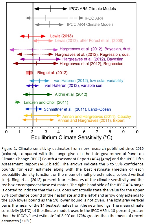
A comparison to various past estimates of ECS is made in figure 5. The base for figure 5 comes from the following weblink :
http://www.cato.org/sites/cato.org/files/wp-content/uploads/gsr_042513_fig1.jpg
See link for the original figure.

Figure 5 : Comparison of the results of this study (1.8) to other recent ECS estimates.
The estimate derived from this study agrees very closely with other recent studies. The gray line on figure 5 at a value of 2.0 represents the mean of 14 recent studies. Looking at the MSE curve in figure 4, 2.0 is essentially flat with 1.8 and would have a similar probability. This study further reinforces the conclusions of other recent studies which suggest climate sensitivity to CO2 is low relative to IPCC estimates .
The big difference with this study is that it is strictly based on the observed data. There are no models involved and only one assumption – that the longer period variation in temperature is driven by CO2 only. Given that the conclusion of a most likely sensitivity of 1.8 ° C / doubling is based on 163 years of observed data, the conclusion is likely to be quite robust.
A brief discussion of the assumption will now be made in light of the conclusion. The question to be asked is : If there are other factors affecting the long period trend of the observed temperature trend (there are many other potential factors, none of which will be discussed in this paper), what does that mean in terms of this best fit ECS curve ?
There are 2 options. If the true ECS is higher than 1.8, by definition , to match the observed data, there has to be some sort of negative forcing in the climate system pushing the temperature down from where it would be expected to be. In this scenario, CO2 forcing would be preventing the temperature trend from falling and is providing a net benefit.
The second option is the true ECS is lower than 1.8. In this scenario, also by definition, there has to be another positive forcing in the climate system pushing the temperature up to match the observed data. In this case CO2 forcing is smaller and poses no concern for detrimental effects.
For both of these options, it is hard to paint a picture where CO2 is going to be significantly detrimental to human welfare. The observed temperature and CO2 data over the last 163 years simply doesn’t allow for it.
Conclusion :
Based on data sets over the last 163 years, a most likely ECS of 1.8 ° C / doubling has been determined. This is a simple calculation based only on data , with no complicated computer models needed.
An ECS value of 1.8 is not consistent with any catastrophic warming estimates but is consistent with skeptical arguments that warming will be mild and non-catastrophic. At the current rate of increase of atmospheric CO2 (about 2.1 ppm/yr), and an ECS of 1.8, we should expect 1.0 ° C of warming by 2100. By comparison, we have experienced 0.86 ° C warming since the start of the HADCRUT4 data set. This warming is similar to what would be expected over the next ~ 100 years and has not been catastrophic by any measure.
For comparison of how unlikely the catastrophic scenario is, the IPCC AR5 estimate of 3.4 has an MSE error nearly as large as assuming that CO2 has zero effect on atmospheric temperature (see fig. 4).
There had been much discussion lately of how the climate models are diverging from the observed record over the last 15 years , due to “the pause”. All sorts of explanations have been posited by those supporting a high ECS value. The most obvious resolution is that the true ECS is lower, such as concluded in this paper. Note how “the pause” brings the observed temperature curve right to the 1.8 ECS synthetic record (see fig. 3). Given an ECS of 1.8, the global temperature is right where one would predict it should be. No convoluted explanations for “the pause” are needed with a lower ECS.
The high sensitivity values used by the IPCC , with their assumption that long term temperature trends are driven by CO2, are completely unsupportable based on the observed data. Along with that, all conclusions of “climate change” catastrophes are also completely unsupportable because they have the high ECS values the IPCC uses built into them (high ECS to get large temperature changes to get catastrophic effects).
Furthermore and most importantly, any policy changes designed to curb “climate change” are also unsupportable based on the data. It is assumed that the need for these policies is because of potential future catastrophic effects of CO2 but that is predicated on the high ECS values of the IPCC.
Files:
I have also attached a spreadsheet with all my raw data and calculations so anyone can easily replicate the work.
ECS Data (xlsx)
=============================================================
About Jeff:
I have followed the climate debate since the 90s. I was an early “skeptic” based on my geologic background – having knowledge of how climate had varied over geologic time, the fact that no one was talking about natural variation and natural cycles was an immediate red flag. The further I dug into the subject, the more I realized there were substantial scientific problems. The paper I am submitting is a paper I have wanted to write for years , as I did the basic calculations several years ago & realized there was no support in the observed data for high climate sensitivity.
This simplistic and faulty analysis assumes that the Hadrut temperature record is a true representation of World temperatures over the period shown. In fact, the Hadcrut graph, like all similar ones is the result of continuous ‘adjustment’ to increase recent temperatures and reduce past temperature records. Most recent temperature increases are solely the result of beneficial ‘adjustments’.
Basing a comparison and sensitivity between CO2 levels and temperature also assumes that there are no other influences at all (like the Sun) on Earth’s average temperature. Coming up with a figure of 1.8 or the IPCC 2.1 or the alarmist 4 is just folly.
First one has to establish what are the real influences on Earth temperature and then work back to their likely effects, not assume that it is just CO2 and attribute ‘adjusted’ temperature rise to that.
REPLY: Then go do it, but in the meantime your comment is little more than whining – Anthony
Simple and elegant.
Thermal mass seems to be ignored.
You can’t calculate an equilibrium value without a thermal mass unless you assume the thermal mass is negligible – making the instantaneous value the equilibrium value. Considering the amount of water on the planet, it seems unlikely that the thermal mass of the planet is negligible.
And, of course, the oceans move heat spatially and temporally. The simplest acceptably accurate solution to a problem is definitely the best one, but this solution is too simple, too inaccurate.
The assumption relating to climate sensitivity to carbon dioxide is dependent upon an assumption that there would be uniform temperatures in the troposphere in the absence of moisture and so-called greenhouse gases. GH gases are assumed to establish a “lapse rate” by radiative forcing and subsequent upward convection.
In physics “convection” can be diffusion at the molecular level or advection or both. It is important to understand that the so-called “lapse rate” (which is a thermal gradient) evolves spontaneously at the molecular level, because the laws of physics tell us such a state is one with maximum entropy and no unbalanced energy potentials. In effect, for individual molecules the mean sum of kinetic energy and gravitational potential energy is constant.
So this thermal gradient is in fact a state of thermodynamic equilibrium. If it is already formed in any particular region then indeed extra thermal energy absorbed at the bottom of a column of air will give the impression of warm air rising. But that may not be the case if the thermal gradient is not in thermodynamic equilibrium and is initially not as steep as it normally would be. In such a case thermal energy can actually flow downwards in order to restore thermodynamic equilibrium with the correct thermal gradient.
What then is the “correct” thermal gradient? The equation (PE+KE)=constant amounts to MgH+MCpT=constant (where M is the mass, H is the height differential and T the temperature differential and Cp the specific heat.) So the theoretical gradient for a pure non-radiating gas is -g/Cp as is well known to be the so-called dry adiabatic lapse rate. However, thermodynamic equilibrium must also take into account the fact that radiation could be transferring energy between any radiating molecules (such as water vapour or carbon dioxide) and this has a propensity to reduce the net result for the thermal gradient. Hence we get the environmental lapse rate representing the overall state of thermodynamic equilibrium.
This can’t be! The data agrees with the conclusions! (sarc off)
The simple fact is this; warmists believe that traces of CO2 generated at ground level by the burning of so called “fossil fuels” make the implausible journey to the upper atmosphere and cause CAGW – they have NO other position whatsoever, and since despite their mantra and models, recent GW has ceased for 17.5 years, they have NO position whatsoever.
Case proven and closed, time to get a real job and stop wasting the taxpayers money!
Good work. But the assumption that I find almost universal and, to my mind, the most unlikely, is that CO2 emissions will continue at the current rate. Look at the full range of assumptions
that simple assumption requires : that electric cars will not replace current ICE vehicles for many decades; that electricity will not be increasingly produced by non-CO2 emitting generators (especially nuclear, which is experiencing unprecedented adoption in India, China, the Middle East, South America, Britain, etc, places where a large portion of the CO2 emission sources are located), that natural gas will not continue to replace most coal generation, or alternatively, that the non-emitting coal combustion process developed at Ohio State will not become commercialized).
That CO2 emissions will remain the same for the extended future I find utterly implausible and
practically impossible. Time and technology marches on. Always has, always will.
ntesdorf: I suppose if you find the analysis simplistic and faulty, you might as well criticize it on the same basis, which you seem to have done quite nicely.
[snip – waaaaaaaaaaayyy off topic – Anthony]
I always suspect calculations based on 100 plus years which eliminates the historical earth climate. Other warm periods in time plus the various ice ages. However I do understand in the AGW camp CO2 as THE factor. What I don’t get is why we always fall into the AGW trap and only concentrate what the AGW camp wants us to talk about, CO2. Something melted each ice age long before man ever existed. I know, I know – trying to prove man is entirely responsible is the buzz words. With respect – I don’t trust any temperature massaged so many times none of us know what real temperature were or supposed to be anymore. Even the different data collected by different device cannot agree with each other and have to be massaged.
Well, setting aside the raging debate on the credibility of the data set being used, this is assuming that ALL influences on global temperature are solely attributable to carbon dioxide concentrations, which I presume most sincere people would doubt. However, as a tact to take while in a bar debating the severity of anthropogenic global warming, I fully support its simplicity in pointing out the flaws of an alarmist’s argument for catastrophe.
I hate to be the guy throwing cold water, but that method needs to be tested on out-of sample data. All you’ve done up there is a simple fit of CO2 to temperature. I can do the same thing with the cost of US postage stamps, and get the same level of significance. Or I can do it with population, or with the cumulative inflation rate … so what?
As a first test of your results, you need to do an “out-of-sample” test by doing the following:
1. Divide your data into 3 periods of ~ 50 years each.
2. Fit the CO2 increase to the temperature in each of the periods separately.
3. Apply the “climate sensitivity” you found in step 2 to the other two segments of the data and note how poorly they fit.
Give that a shot, report back your results …
w.
‘In general, those who are supportive of the catastrophic hypothesis reach their conclusion based on global climate model output.”
Wrong. Hansen for example relies on Paleo data.
REPLY: and I call BS on your “wrong”
From Hansen’s “paper”:
Hansen, J., 2007: Climate catastrophe. New Scientist, 195, no. 2614 (July 28), 30-34.
A sea level rise of several metres will be a near certainty if greenhouse gas emissions keep increasing unchecked. Why are scientists reluctant to speak out? http://pubs.giss.nasa.gov/docs/2007/2007_Hansen_2.pdf
– Anthony
“Hansen for example relies on Paleo data.”
But who relies on Hansen? Anyone? [I mean, anyone rational.]
Here’s Siple vs Mauna Loa. I wouldn’t be surprised if Law Dome has also been faked.
http://www.ferdinand-engelbeen.be/klimaat/klim_img/siple1a.jpg
I saw no formulas in the “modeled temps” tab of your spreadsheet, but I infer from your discussion that you assumed no delay. My understanding of “equilibrium climate sensitivity” is the temperature increase that results after the C02 concentration has reached double and remained there indefinitely.
In other words, proponents of high equilibrium client sensitivity would say that temperatures would continue to climb even if CO2 concentration remained fixed; it would approach the equilibrium value asymptotically.
This means you need at least two parameters (only two if you assume a first-order linear system): equilibrium climate sensitivity and time constant, or, as vboring put it, thermal mass.
The article ignors the fact that CO2 changes are a result of warming rather than a cause.
A perfectly reasonable analysis as far as it goes. It suffers from the usual — the assumption that CO_2 is the only knob is almost certainly false. For example, would anyone care to take the model and hindcast the Little Ice Age from it? How about the Medieval Warm Period? We know that the climate varies naturally by order of 1 C or more on a century time scale. Indeed, if one looks even at HADCRUT4:
http://www.woodfortrees.org/plot/hadcrut4gl/from:1800/to:2013/plot/hadcrut4gl/trend
The rule rather than the exception is for the climate to vary by 0.1C or more over a decade. Furthermore, the rule rather than the exception is for the climate to vary by 0.1/decade or more over multiple decades in a row in a single direction.
How anyone could call the stretch from 1970 to 2000 “unusual” is beyond me, when the stretch from 1910 to 1940 is almost identical in structure and span.
Note well that CO_2 did not descend or remain neutral from 1855 to 1910, or from 1950 to 1970, or from 2000 to the present, but the climate did.
Basically, one simply cannot look at the temperature record anywhere and ascertain how much of any given stretch of temperature or its variation occurs due to “natural” causes and how much occurs due to variations in atmospheric GHG chemistry. No simple model fits (even when reasonably well done, as this one is) can accomplish it. Neither, apparently, can predictive models.
rgb
It seems to me there is a fundamental mental error being made if one considers the ECS as anything but the net end result. The author discusses the possibilities of a high ECS with negative forcings keeping temperatures lower, and a low ECS with positive forcings keeping temperatures elevated. I see the ECS as the final result of all the forcings, negative and positive, on the global temperature. If the temperature and CO2 observations suggest a value of 1.8, then that is the true value. Period. The end.
In a complex system like the climate, wouldn’t all of the myriad variables and forcings mingle to determine how the climate reacts to increased CO2, and then that would BE the ECS? Maybe I’m seeing it wrong, and I would certainly appreciate seeing where I’ve made my error.
The problem with this analysis is that it assumes that all warming is caused by CO2, which is obviously wrong when viewing the HADCRUT plot. There is clearly a natural components which caused warming in early 1900s, and some cooling 1940-1970. It is faulty logic to make an assumption that is wrong, and then declaring that if there is a natural component then the situation is even better. In fact, addition of a natural component that suggests a higher ECS, is not a good thing because we don’t know what are the future natural drivers to the climate. There may be in the future natural warming added to CO2 forcing.
So the error here is that we are suggesting we know something, when in fact we don’t. We face an unquantified future risk (it may be bad, it may not be). When we acknowledge this uncertainty, it is wrong to be panicking and declaring that we face certain doom unless we dismantle our energy technology base, but fooling ourselves into believing everything is OK is also self-deceit.
I would encourage the author of this essay to do the analysis again for a range of assumptions of natural climate change vs CO2 forcing see what results. Instead of pinning down a value for ECS, I suggest it would probably result in a wide range of values. But I believe it would be a worthwhile venture, if only to show the impact of assumptions of natural vs human induced in this debate.
“The big difference with this study is that it is strictly based on the observed data. There are no models involved and only one assumption – that the longer period variation in temperature is driven by CO2 only.”
Well there MUST be some natural variability in there as well. So the figure could be lower (or higher) than that quoted.
http://i29.photobucket.com/albums/c274/richardlinsleyhood/Fig8HadCrutGISSRSSandUAHGlobalAnnualAnomalies-Aligned1979-2013withGaussianlowpassandSavitzky-Golay15yearfilters_zps670ad950.png
1. to calculate ECS you have to include OHC ( or assume) that OHC is zero.
in other words, ECS implies that the system has reached equillibrium. So since the
system has not, you need to have an estimate for delta OHC.
2. If you do not include delta OHC, then you are estimating something closer to TCR
TCR is roughly 1.3 to 2.2 so your estimate is in line with this
Next, to do the estimate properly you need all Forcing
use all forcing to give you lambda.. the system response to all forcing
from lambda you can calculate the senitivity to C02 doubling
I concur with what Willis stated, but I propose you take your simple analysis a little further. Show us a graph of the deviation of the “actual” temperature record from the “1.8” calculated record, then calculate the simple statistical values that determine the “cause/effect” certainty of your “model”. Second, you need to turn the whole concept on it’s head and ask the question, does the temperature record cause the CO2 change instead of vice versa. Others have proposed and documented with a fair degree of certainty that the integral of the actual temperature trends predict the current CO2 values.
IMHO temperature drives CO2 increase and the burning of fossil fuels is dwarfed by simple outgassing from the integral effect of accumulated ocean warming. More importantly than that, you are falling into the trap of arguing about the “noise” when in fact on any given day/month/year temperature changes far above 1 or 2 degrees in spite of a relatively CONSTANT CO2. There is NO temperature signal at Mauna Loa that matches the annual cyclical CO2 concentration signal!
There are a number of factors of unknown magnitude that render any attempt to derive the right value of sensitivity in the manner done here essentially impossible.
To begin with, a proper model must recognize that the real Earth has thermal inertia. This means, at the very least, one needs to use a differential equation of the form:
T = sensitivity*Forcing -response time*dT/dt
The second problem is that one needs to recognize that more forcings other than CO2 act on the temperature record. These include volcanic eruptions, variations in solar brightness, other greenhouse gases (such as methane, CFCs, N2O, etc), dynamically induced non feedback variations in cloud cover, sulphates, black carbon, land use change, and many, many more factors, most of which are highly uncertain.
The third problem is uncertainty of the temperature record itself-how much of the change is real versus due to data biases?
The fourth problem is non linearity of sensitivity-that is, df/dT, where f represents the rate of radiative heat loss, is not a constant, as various effects can increase or decrease the change of rate with temperature at higher temperatures.
All of these problems make attempting to estimate the sensitivity in this way pretty much a pointless exercise. Something that would make more sense would be to attempt to estimate the magnitude of the feedback response, which overcomes every problem except the fourth.
Of course, if you do that, you’re going to get an answer that’s like a third what you’re getting here. But given all the problems with this approach, that’s not that surprising.
The most significant evidence we have of low sensitivity is the pause. The alarmist need the heat to be in the ocean. They need it or they know it is game over.
If we have perfect measurements from satellites of the input and output heat radiation budget then we will know if heat is in ocean.
My guess is that there is a big negative feedback mechanism we do not fully understand. There is some type of release valve , throttle as Willis says. It has to do with water cycle or wind in my opinion.