 (Perturbation Calculations of Ocean Surface Temperatures.)
Guest essay by Stan Robertson, Ph.D., P.E.
1. Introduction
It is generally conceded that the earth has warmed a bit over the last century, but it is not clear what has caused it, nor whether it will continue and become a problem for humanity. There is a possibility that some of the warming has been caused by anthropogenic greenhouse gases, but it is also likely that the sun has been partially responsible. The arguments that are advanced to say that humans caused it and that it will become a serious problem rely on models that have not been validated and positive feedback effects that have not been shown to exist, at least at the hypothesized levels of effectiveness. The apparent weakness in the argument that the sun has been a major contributor is that satellite measurements of Total Solar Irradiance (TSI) have not shown changes large enough to have directly produced the warming of the earth over the last half century. But what about indirect effects? Is it possible that the sun exerts control in some indirect way? In these notes I recapitulate the evidence that this is the case by showing that the variations of TSI cannot provide the energy that is necessary to account for the warming of the oceans during solar cycles.
TSI, as measured above the earth’s atmosphere varies by about 1.2 watt/m2 over a nominal eleven year solar cycle (h/t Leif Svaalgard) primarily at wavelengths shorter than 2 micron. The dominant harmonic variation of TSI would thus have an amplitude half this large, or about 0.6 watt/m2. About 70% of this enters the earth atmosphere. Averaged over latitudes and day/night cycles, about one fourth of this 70%, or ~0.11 watt/m2, on average, enters the upper atmosphere. Since only about 160 watt/m2 of 1365 watt/m2 of incoming solar radiation at wavelengths less than 2 micron reaches the earth surface, the amplitude of short wavelength TSI reaching the earth surface would be only (160/1365)x0.6 = 0.07 watt/m2. However, about half of the difference between 0.11 and 0.07 watt/m2 eventually reaches the earth surface as scattered thermal infrared radiation at wavelengths greater than 2 micron. Thus the average amplitude of TSI reaching the earth surface in all wavelengths would be about 0.09 watt/m2. So the question is, just how much sea surface temperature variation can this produce?
Several researchers, including Nir Shaviv (2008), Roy Spencer (see http://www.drroyspencer.com/2010/06/low-climate-sensitivity-estimated-from-the-11-year-cycle-in-total-solar-irradiance/) and Zhou & Tung (2010) have found that ocean surface temperatures oscillate with an amplitude of about 0.04 – 0.05 oC during a solar cycle. (In fact, all of the ideas that I am presenting here were covered in Shaviv’s work, but it has not gotten the attention that it deserves.) Using 150 years of sea surface temperature data, Zhou & Tung found 0.085 oC warming for each watt/m2 of increase of TSI over a solar cycle. Although not strictly sinusoidal, the temperature variations can be approximately described in terms of a dominant sinusoidal component of variation with an 11 year period. Thus the question to be answered at this point is, can 0.09 watt/m2 amplitude of variation of TSI entering the oceans produce temperature oscillations with an amplitude of 0.04 – 0.05 oC?
The answer to this question depends on the average thermal diffusivity of the upper oceans. That is an unknown, but not unknowable, quantity. Thermal diffusivity is the ratio of thermal conductivity to heat capacity. The upper 25 to 100 meters of oceans are well mixed by waves and shears. These are mixing zones with high thermal diffusivity and correspondingly small temperature gradients. Diffusivities are lower at greater depths. Bryan (1987) has found that thermal diffusivities ranging from 0.3 to 5 cm2/s are needed to account for the temperature profiles below the mixing zone. In my first trial calculations of the energy flux necessary to account for the temperature variations, I tried values of thermal diffusivity in the range 0.1 – 10 cm2/s and found that the TSI variations were generally inadequate to produce the sea temperature variations over a solar cycle. But there was wide variation of calculated energy flux. Larger values of thermal diffusivity required more heat because more was able to penetrate to the depths, but even for 0.1 cm2/s, the required input was double the TSI variations that reach the earth surface. Fortunately, there is a way to constrain both the value of the thermal diffusivity and the heat input. It consists of first matching the measured trends of surface temperatures and ocean heat content over time. Measurements of these were reported by Levitus et al. (2012) and are available from http://www.nodc.noaa.gov/OC5/3M_HEAT_CONTENT/ .
In the calculations described below, I have used the data from 1965 to 2012 for ocean depths to 700 meters. Sea surface temperatures and ocean heat content began to increase after 1965. Only about a third of the increase of heat content occurred at depths below 700 meter. Since little heat migrates below this depth over 11 year solar cycles, it is preferable to use the 0 – 700 m data for the purpose of calibrating the thermal diffusivity
2. Heat Transfer Perturbation Calculations
For the calculation of sea surface temperature and sea level changes, we can treat the variations of radiations entering and leaving atmosphere, lands and oceans as minor perturbations on an earth essentially in thermal equilibrium. Ocean mixing zones, thermoclines and other features of the temperature profiles remain largely as they were while small radiant disturbances produce minor variations of temperature starting from zero, and imposed at each depth. Thus the effects of these disturbances can be modeled as one-dimensional energy flows into a medium at uniform temperature. Such “perturbation calculations” are among the most powerful analysis techniques used by physicists and engineers and are widely used. The energy equation to be solved in this case is:
http://i1244.photobucket.com/albums/gg580/stanrobertson/equation_zpscea297ad.jpg

Where T is the temperature departure from equilibrium at depth , z, and time, t. q is a perturbing radiant flux entering the surface, u the absorption coefficient, c is absorber heat capacity and k its thermal conductivity. The rate of heat transfer by conduction processes is controlled by the thermal diffusivity, which is the ratio k/c.
As a one dimensional heat flow problem, it is straightforward undergraduate level physics or engineering to numerically solve the equation above for the expected changes of surface temperature as surface radiant flux varies. In my calculations, temperature changes were calculated for 1.0 meter increments of depth in the oceans. Two cases were considered. In one
case the surface radiation perturbation was assumed to increase linearly with time. This corresponds to the ocean conditions for the period 1965-2012. In the second case, it was assumed to vary as a cosine function of time with the 11 year period of the solar cycle. The cosine function provides both some positive and some negative variation in the first half cycle, which helps to minimize the transients of the first few years.
I treated q and thermal diffusivity, (k/c), as input parameters that were chosen to provide agreement with the observed sea surface temperature variations and ocean heat content measurements (https://www.ncdc.noaa.gov/ersst/ ). The absorption coefficient, u, was entered in piecewise fashion. Only the deep UV radiations penetrate to depths below 10 meter, but conduction takes energy to much greater depths. For the values of u chosen, only 44.5% of the surface energy flux goes deeper than 1 meter, 22.5% below 10 meter and 0.53% to 100 meter (h/t Leif Svalgaard). Thermal diffusivity of oceans was assumed to be 0.3 cm2/s below 300 m. This accords with Bryan’s estimates below the mixing zone, but little change of results occurred for values as low as 0.1 cm2/s. The required heat inputs are relativity insensitive to the thermal diffusivity below 300 meter. For the shallower depths, thermal diffusivity was varied until trends in accord with observed temperatures and heat content were produced.
It is necessary to maintain an energy balance at the sea surface in approximate equilibrium with the incoming solar radiation. As estimated by Trenberth, Fasullo and Kiehl (2009), about 160 watt/m2 enters the surface, on average. At a mean temperature of 288 oK, the sea surface will emit about 390 watt/m2 of surface thermal infrared radiation at wavelengths longer than about 2 micron, however, about 84% of that is returned as back scattered radiation. The rest of the energy balance is provided by evaporation and thermal convection, which remove about 59% of the heat from the surface. From the standpoint of merely wanting to know how much heat is required to change the ocean surface temperature, it is possible to maintain a proper energy balance without delving into the messy details of evaporation, convection and infrared absorption in the first few millimeters of water. The temperature variations at one meter depth will not be measurably different from those at the surface for the thermal diffusivities of interest here. If we merely want to know what net energy flux entering the surface is required to make the water temperature at one meter depth oscillate with an amplitude of 0.04 – 0.05 oC , then all we need to do is account for the outgoing surface infrared emission and let 41% (160 watt/m2 / 390 watt/m2 = 0.41) escape. At the present 288 oK, the earth radiates an additional 5.42 watt/m2 for each 1 oC increase of surface temperature. In the case of surface temperature being perturbed by 0.04 oC, an outgoing additional 0.22 watt/m2 would be generated and 0.09 watt/m2 was allowed to escape. This nicely balances the amplitude of TSI variations that reach the earth’s surface.
3. Linear heating:
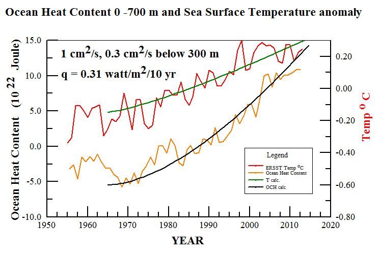
In these calculations, the aim was to find the heat input and thermal diffusivities necessary to account for the observed surface temperature increase (http://www.nodc.noaa.gov/OC5/3M_HEAT_CONTENT/ )Extended Reconstructed Sea Surface Temperature) and the increased ocean heat content (OHC 700) that have been reported by NOAA. Since surface temperatures had not been increasing in the early 1960s, but began to increase in the last half of that decade, I chose to start calculations with linearly increasing heating in 1965. I found that the ocean heat content to a depth of 700 meters was quite sensitive to the thermal diffusivity used. The best results that I have been able to obtain were for a thermal diffusivity of 1 cm2/s to 300 meter depth and surface heat input increasing at a rate of 0.31 watt/m2 per decade. These are shown on the graph below with calculated trends shown by the green and black lines. On a time scale of 50 years, most of the heat accumulates at relatively shallow depths. To better reflect a realistic thermal diffusivity for greater depths, I used a lower value of 0.3 cm2/s below 300 meter. That has little practical effect on a 50 year times scale, but would be necessary if one wanted to extend the calculations for several centuries while surface heating perturbations had time to penetrate to much greater depths.
http://i1244.photobucket.com/albums/gg580/stanrobertson/OHC700_zpsb9e34e91.jpg

Figure 1. Ocean heat content 0 – 700 meter and surface temperature trends according to NOAA. Blue and green lines show trends calculated for the parameters shown.
These calculations establish some parameters that do a good job of representing the thermal behavior of the upper oceans, however, if one looks closely at the data trends in the graph, it is apparent that both surface temperature and ocean heat content have considerably slowed their rates of increase in the last decade. This makes it unlikely that greenhouse gases are the cause of the rate of heating needed to explain the previous trends because their effects should have become enhanced rather than diminished. It might also be noted that a similar warming trend occurred in the first half of the previous century before anthropogenic greenhouse gases could have contributed significantly. Thus it is more likely that both warming periods had natural origins.
Obtaining simultaneous fits to the ocean heat content and sea surface temperature trends with only two free parameters, thermal diffusivity and surface heating rate, is quite confining. Acceptable, but noticeably worse, fits than shown above, were obtained with thermal diffusivities ranging from 0.8 to 1.2 cm2/s and heat inputs ranging from 0.29 to 0.33 watt/m2. Based on previous calculations for sea level data, I was initially inclined to think that larger thermal diffusivities would be necessary, but larger values let more heat penetrate to greater depths than the amounts of heat reported by Levitus et al. In addition, I was chagrined to learn that most of the variation of sea level that accompanies solar cycles is caused by evaporation rather than thermal expansion.
Solar Cycles:
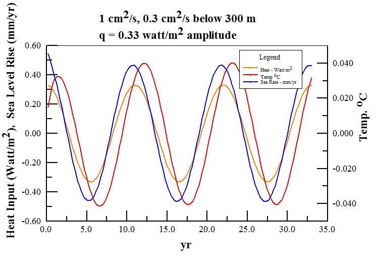
The process of choosing thermal diffusivity and surface heating rates to accord with observations provides a sound basis for calculating what to expect for the temperature variations during solar cycles. In this case we can use the thermal diffusivity of 1 cm2/s that is required of the ocean heat content results as an input parameter and choose the heat input that is required to produce temperature variations of 0.04 – 0.05 oC amplitude. Producing sea surface temperature variations with an amplitude of 0.04 oC requires a surface heat input of 0.33 watt/m2, as shown below:
http://i1244.photobucket.com/albums/gg580/stanrobertson/solarcycle10_zpsa3b8b0ee.jpg

Figure 2. Radiant flux, ocean temperature oscillations, and sea level variations for three solar cycles of eleven years each. The entering flux shown here is the value of q = 0.33 watt/m2 needed to drive the variations of surface temperature of 0.04 oC with ocean thermal diffusivity of 1.0 cm2/s to depth of 300 m. The amplitude of thermosteric rate of change of sea level was 0.47 mm/yr. Temperature lags the driving energy flux by 15 months. The thermal expansion coefficient of sea water used here was 2.4×10⁻⁴/ oC.
I believe that this settles the issue of what is required to produce sea surface temperature oscillations with an amplitude of 0.04 oC. The solar TSI variations that reach the earth’s surface are smaller than the 0.33 watt/m2 needed to account for sea surface temperature variations by a factor of 3.6 for this smallest estimate of sea surface temperature variability.
Although the estimated 0.33 watt/m2 that is required to explain the surface temperature variations is large compared to the amplitude of TSI variations that reach the surface, it is still only about two parts per thousand of the 160 watt/m2 of solar UV/VIS/NIR that reaches the earth surface. There are many possible ways in which the sun might modulate the surface energy flux to this extent. These include modulation of cloud cover and small spectral shifts in the energetic UV that might modulate ozone absorption or produce shifts of the effective sea surface albedo. It would seem to be a fairly direct radiative effect, rather than feedback, since it must vary in phase with the solar cycle.
In summary, my calculations based on energy conservation considerations imply that the sun modulates the ocean temperatures to a much greater extent than can be provided solely by its TSI variations. The great question that desperately needs an answer is how does it do it? It should be easily understood that solar effects would not necessarily be confined to cycles. More likely, the sun has been the driver of the large changes of temperatures of the Roman and Medieval warm period, the Little Ice Age, and the recent recovery from it without requiring large changes of its own irradiance. When we understand how the sun does this, we will have begun to understand the earthly climate.
###
Biographical note:
Stan Robertson, Ph.D, P.E, retired in 2004 after teaching physics at Southwestern Oklahoma State University for 14 years. In addition to teaching at three other universities over the years, he has maintained a consulting engineering practice for 30 years.
References:
Bryan, F., 1987: Parameter Sensitivity of Primitive Equation Ocean General Circulation Models. Journal of Physical Oceanography, 17, 970-985. (PDF available here http://journals.ametsoc.org/doi/abs/10.1175/1520-0485%281987%29017%3C0970%3APSOPEO%3E2.0.CO%3B2
Levitus, S. et al., 2012 World ocean heat content and thermosteric sea level change (0–2000 m), 1955–2010, Geophysical Research Letters, 39, L10603, doi:10.1029/2012GL051106, 2012 http://onlinelibrary.wiley.com/doi/10.1029/2012GL051106/abstract
Shaviv, Nir 2008, Using the oceans as a calorimeter to quantify the solar radiative forcing, Journal of Geophysical Research, 113, A11101 http://www.sciencebits.com/files/articles/CalorimeterFinal.pdf
Trenberth, K., Fasullo, J., Kiehl, J. 2009: Earth’s Global Energy Budget. Bull. Amer. Meteor. Soc., 90, 311–323. doi: http://dx.doi.org/10.1175/2008BAMS2634.1 www.cgd.ucar.edu/staff/trenbert/trenberth.papers/TFK_bams09.pdf , Fig. 1
Zhou, J. and Tung, K. ,2010 Solar Cycles in 150 Years of Global Sea Surface Temperature Data, Journal of Climate 23, 3234-3248 http://journals.ametsoc.org/doi/abs/10.1175/2010JCLI3232.1
It’s a chaotic system, Leif. Do you claim to know all the inputs and perturbations, and their eventual manifestations? Small perturbations can be magnified by impacting the development of larger scale systems. Jerry Browning showed that in the upward cascade of enstrophy in atmospheric gyres.
The UV radiation of the sun varies wildly, add in the Forbush events, cosmic rays, cloud formation and there is plenty there to tie solar variations to climate cycles.
mem says:
October 10, 2013 at 6:02 pm
If I may quibble with the good Dr. Abdusamatov, IMO the term “Little Ice Age” should be reserved for the longer cold period from c. 1250-1400 to c. 1850, ie roughly half a Bond Cycle. Within both centennial-length warm & cold “periods” of course occur shorter counter-trend cool or warm phases. By analogy with financial market history, there are secular trends (hundreds of years in the case of climate), with cyclical counter trends (decadal) within them.
The sun may influence both the secular & cyclical trends, but oceanic circulation is clearly associated with the decadal fluctuations.
The bicentennial TSI effect Abdusamatov claims to have found fits in well with this quasi-periodic pattern. At the risk of being labeled a cyclomaniac, I’ll say that IMO it appears real, not spurious: decades ruled by oceanic oscillations, with longer, bicentennial cycles under TSI influence, which add up to semi-millenial waves (half Bond Cycles), all superimposed to produce the quasi-ness of it all until a new glaciation begins & the weak Bond Cycles become powerful Dansgaard-Oeschger Cycles (Dansgaard being another recently late, great Dane).
Tibet & Okinawa pick up the solar signal:
http://onlinelibrary.wiley.com/doi/10.1029/2011JD017290/abstract
http://www.agu.org/pubs/crossref/pip/2012GL052749.shtml
It’s unicorns Leif.
Steve mosher says:
October 10, 2013 at 6:38 pm
The unicorns are inflated by CO2.
The may sun rule, even if humans don’t know how yet. Climate is complex, possibly even chaotic. But what it isn’t is CO2 & nothing else, as per the IPeCaC fantasy. Mother Nature has already slapped down that delusion, as she already had long before the gaseous madness was ever even promulgated by the raving loon Hansen.
Pat Frank says:
October 10, 2013 at 6:29 pm
It’s a chaotic system
Even chaos cannot make 36 W/m2 out of 10 W/m2.
The Sun was more than averagely active all the way from 1934 to 2003, and although the peak amplitudes fell gently after 1958 (not forgetting the 20% Waldmeier overcount Leif won’t mention in this sort of thread), the minima were brief and the cycles short and steep.
So given that there will be an average sunspot number at which the oceans neither gain nor lose energy (give r take some cloud variation (also solar linked), and given the thermal inertia of the millions of cubic kilometres of water in the upper oceans, would we expect:
The OHC to rise from 1934 to 1960 and then fall
The OHC to rise for as long as the Sun remained more than averagely active
The OHC to leap about at a moments notice in response to the ups and downs of 11 year solar cycles as Leif demands?
Ocean temps, surface temps, ENSO, etc., they are all reactions not causes.
Perhaps TSI variation is enough to effect thermal convection to space.
tallbloke says:
October 10, 2013 at 6:56 pm
So given that there will be an average sunspot number at which the oceans neither gain nor lose energy
That is not a given. The oceans gain energy every day no matter what the sunspot number is and lose what they have gained again at night. Over the long run, the average ocean temperature will just depend on the average incoming solar radiation. If the solar incoming were to go up [because of more sunspots] the ocean temperature will go up. If the incoming stayed at its higher level the ocean temperature the ocean would stay at its higher temperature [i.e. neither gain nor lose energy] even though the sunspot number is higher, so now it will at a different average sunspot number that the oceans will neither gain nor lose energy, so here is no fixed ‘magic sunspot number’ involved.
Hand-waving, Leif. How do you know that small perturbations don’t affect larger scale energy transfer between coupled oscillating climate systems?
Does the proportion of IR, visible light and UV vary enough in the measured TSI to cause a change in heat received at the surface ? So if the total TSI variation is insignificant, are the wave length contributions to TSI constant.?
Leif Svalgaard says:
(quote Robertson) The solar TSI variations that reach the earth’s surface are smaller than the 0.33 watt/m2 needed to account for sea surface temperature variations by a factor of 3.6 for this smallest estimate of sea surface temperature variability.
So, in normal science, that falsifies the assumption that solar variations are the cause.
———————————————————-
I agree with Leif that intrinsic solar variations are not the cause. Something within the atmosphere causes the variations at the sea surface and it might even be merely a coincidence that higher temperatures and TSI just happen to vary in phase with some other driving mechanism. But the fact that the sun is the ultimate cause is shown by the same periodicity for the TSI and earth surface temperature cycles
Leif knows very well that TSI refers to the variation of intrinsic solar radiance that is received at the location of the top of earth’s atmosphere. Like the ordinary 160 watt/m^2 that reaches the ground of about 1365 watt/m^2 incident on the sunny side of the top of the atmosphere, about 160/1365 of that 0.6 watt/m^2 amplitude of TSI will reach the ground as ordinary sunlight. That is 0.07 watt/m^2 at wavelengths below about 2 micron. Another 0.02 watt/m^2 arrives as scattered thermal infrared, making about 0.09 watt/m^2 the part of TSI that enters the surface.
The rest is a very simple physics proposition. We are talking about heating water here. How much heat does it take to heat the oceans to the extent shown? A lot more than 0.09 watt/m^2. Where does it come from? Obviously from the sun, since it varies with the solar cycle period.
But it doesn’t have to be extra heat that entered the top of the atmosphere. The surface oscillations could be caused by extra clouds blocking sunshine from entering for part of the solar cycle. All that we see at the surface are the energy variations, but we do at least know that when TSI is high, the temperature is high, with only a little over a year thermal lag.
Stan Robertson
@OP — ” … imply that the sun modulates the ocean temperatures to a much greater extent than can be provided solely by its TSI variations.”
Since the specific wavelengths matter, looking at TSI doesn’t. Which is the entire discussion behind AGW and GHG’s in the first place.
Pat Frank says:
October 10, 2013 at 7:17 pm
Hand-waving, Leif. How do you know that small perturbations don’t affect larger scale energy transfer between coupled oscillating climate systems?
The article says that 1 W/m2 in gives you 3.6 W/m2 out [actually 0.09 and 0.33, but you should be able to figure that out on your own]. In nature you don’t permanently get something for nothing.
“Although the estimated 0.33 watt/m2 that is required to explain the surface temperature variations is large compared to the amplitude of TSI variations that reach the surface, it is still only about two parts per thousand of the 160 watt/m2 of solar UV/VIS/NIR that reaches the earth surface.”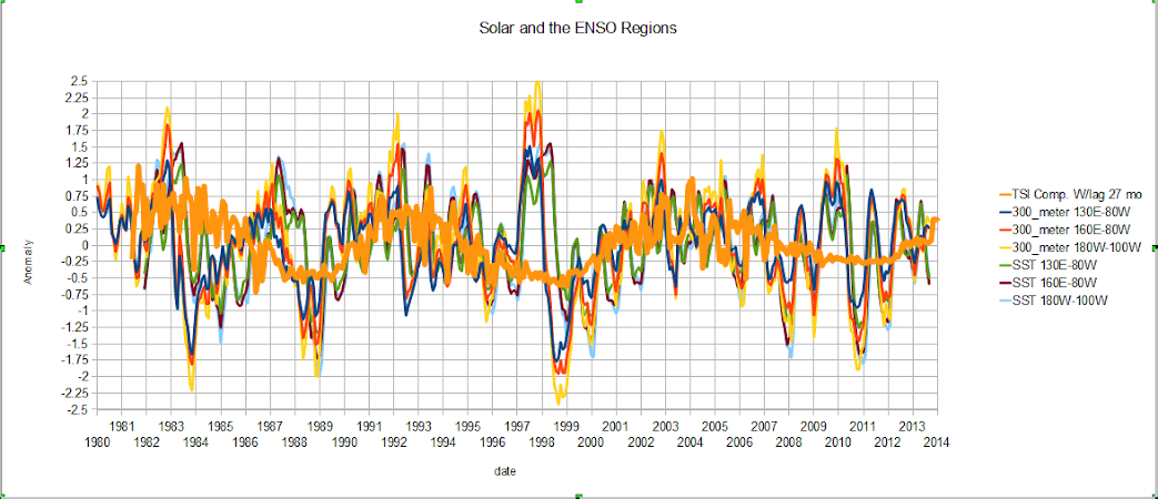
That depends on which surface. If the energy is absorbed near the surface or in the skin layer it is less efficient that if it is absorbed sub-surface in the oceans. The lags are different. For example if you compare the ENSO region with the areas north and south of the ENSO regions you will find a 27 month lag. ENSO lags solar by 27 months at least since 1981 while 30 degrees north and south of the ENSO region are in phase with solar.
I haven’t figure out if that is just a recent thing or not, but it the tropical ocean mixing layer is near equilibrium, you could get some interesting resonance effects. The actual El Nino peaks appear to be a third harmonic. Plus note that for the ocean sub-surface the average insolation should be based on I*cos(theta)/pi() and consider the lag residual as a dc component it appears. Kind of like a liquid greenhouse effect.
Gravitational pull.? Must have some energy input.? Anyone?
Hi. During the day my yard heats up to 19C.
At night it cools to 7 C
Do ya think that the sun has some influence on that?
bones says:
October 10, 2013 at 7:22 pm
The rest is a very simple physics proposition. We are talking about heating water here. How much heat does it take to heat the oceans to the extent shown?
You said: “[people] have found that ocean surface temperatures oscillate with an amplitude of about 0.04 – 0.05 oC during a solar cycle. (In fact, all of the ideas that I am presenting here were covered in Shaviv’s work, but it has not gotten the attention that it deserves.) Using 150 years of sea surface temperature data, Zhou & Tung found 0.085 oC warming for each watt/m2 of increase of TSI over a solar cycle.”
I don’t like your ‘amplitude’ concept as it assumes a given waveform. I prefer the actual valley-to-peak variation, so the numbers become 0.08 to 0.10 C during a solar cycle [for 1.2 W/m2]. Z&T found 0.085 C for 1 W/m2, so average 0.09 C for 1.1 W/m2. Simple physics says S = a T^4, or dS/S = 4 dT/T or dT/T = 1/4 dS/S; with dS = 1.1 and S =1361 and T =289K we find dT = 0.06 K, which is in the ball park of 0.09, so I don’t see the problem.
Looks like the ENSO meter is going negative, this should be interesting considering IPPC says the heat is trapped in the oceans along with an increase in global ice. Here is what is really happening
Perilous Times and Perilous Men
2 Timothy 3
3 But know this, that in the last days perilous times will come: 2 For men will be lovers of themselves, lovers of money, boasters, proud, blasphemers, disobedient to parents, unthankful, unholy, 3 unloving, unforgiving, slanderers, without self-control, brutal, despisers of good, 4 traitors, headstrong, haughty, lovers of pleasure rather than lovers of God, 5 having a form of godliness but denying its power. And from such people turn away!
Such is……….
tallbloke says:
October 10, 2013 at 6:02 pm
OK, so Dr Svalgaard has demonstrated that he doesn’t understand the effect of the thermal inertia of the oceans.
Next!
———————————————————
Touche, tallbloke. It actually takes enough heat to change water temperatures for a few hundred meters below in order to get the surface temperature to change enough. He seems to be content with merely balancing at the surface, but that is physically wrong.
But give him a break. How many solar scientists do you know who would be happy to be told that they don’t understand some a fundamental connection between the sun and earthly climate?
Tallbloke, I follow you perfectly. Amazing how a scientist can just seem to completely ignore the huge mass involved.Your thought of a general null point in the ssn (at best, only an empically aided swag Leif) is precisely how I got involved with wuwt four years ago, yes, that very topic with the charts I sent to Anthony, before I even knew skeptics existed, before I knew there was a raging debate over climate, and curiously Anthony had a post that drew me to his site and he was using that very same happy face sun as the picture on his post “It’s the sun, stupid!”.
Now that is some strange coincidence !! 😉
“c. But what it isn’t is CO2 & nothing else, as per the IPeCaC fantasy.”
Actually C02 forcing is only half the story according to the IPCC.
In short, the science, the IPCC science, attributes the change to MANY forcings. C02 happens to be the largest. Its not the only forcing. However, by the time the science gets politicized its all people talk about.
lsvalgaard says:
October 10, 2013 at 7:41 pm
I don’t like your ‘amplitude’ concept as it assumes a given waveform. I prefer the actual valley-to-peak variation, so the numbers become 0.08 to 0.10 C during a solar cycle [for 1.2 W/m2]. Z&T found 0.085 C for 1 W/m2, so average 0.09 C for 1.1 W/m2. Simple physics says S = a T^4, or dS/S = 4 dT/T or dT/T = 1/4 dS/S; with dS = 1.1 and S =1361 and T =289K we find dT = 0.06 K, which is in the ball park of 0.09, so I don’t see the problem.
————————————————————-
The problem is that your calculation would apply only to a surface with no heat capacity. You are failing to consider the heat required to raise the water temperature for a considerable depth below the surface.
“How do you know that small perturbations don’t affect larger scale energy transfer between coupled oscillating climate systems?”
Prove its not unicorns Pat.
“Gravitational pull.? Must have some energy input.? Anyone?”
yes, it varies with the square root of unicorns.