
Studies of Carbon 14 in the atmosphere emitted by nuclear tests indicate that the Bern model used by the IPCC is inconsistent with virtually all reported experimental results.
Guest essay by Gösta Pettersson
The Keeling curve establishes that the atmospheric carbon dioxide level has shown a steady long-term increase since 1958. Proponents of the antropogenic global warming (AGW) hypothesis have attributed the increasing carbon dioxide level to human activities such as combustion of fossil fuels and land-use changes. Opponents of the AGW hypothesis have argued that this would require that the turnover time for atmospheric carbon dioxide is about 100 years, which is inconsistent with a multitude of experimental studies indicating that the turnover time is of the order of 10 years.
Since its constitution in 1988, the United Nation’s Intergovernmental Panel on Climate Change (IPCC) has disregarded the empirically determined turnover times, claiming that they lack bearing on the rate at which anthropogenic carbon dioxide emissions are removed from the atmosphere. Instead, the fourth IPCC assessment report argues that the removal of carbon dioxide emissions is adequately described by the ‘Bern model‘, a carbon cycle model designed by prominent climatologists at the Bern University. The Bern model is based on the presumption that the increasing levels of atmospheric carbon dioxide derive exclusively from anthropogenic emissions. Tuned to fit the Keeling curve, the model prescribes that the relaxation of an emission pulse of carbon dioxide is multiphasic with slow components reflecting slow transfer of carbon dioxide from the oceanic surface to the deep-sea regions. The problem is that empirical observations tell us an entirely different story.
The nuclear weapon tests in the early 1960s have initiated a scientifically ideal tracer experiment describing the kinetics of removal of an excess of airborne carbon dioxide. When the atmospheric bomb tests ceased in 1963, they had raised the air level of C14-carbon dioxide to almost twice its original background value. The relaxation of this pulse of excess C14-carbon dioxide has now been monitored for fifty years. Representative results providing direct experimental records of more than 95% of the relaxation process are shown in Fig.1.

Figure 1. Relaxation of the excess of airborne C14-carbon dioxide produced by atmospheric tests of nuclear weapons before the tests ceased in 1963
The IPCC has disregarded the bombtest data in Fig. 1 (which refer to the C14/C12 ratio), arguing that “an atmospheric perturbation in the isotopic ratio disappears much faster than the perturbation in the number of C14 atoms”. That argument cannot be followed and certainly is incorrect. Fig. 2 shows the data in Fig. 1 after rescaling and correction for the minor dilution effects caused by the increased atmospheric concentration of C12-carbon dioxide during the examined period of time.

Figure 2. The bombtest curve. Experimentally observed relaxation of C14-carbon dioxide (black) compared with model descriptions of the process.
The resulting series of experimental points (black data i Fig. 2) describes the disappearance of “the perturbation in the number of C14 atoms”, is almost indistinguishable from the data in Fig. 1, and will be referred to as the ‘bombtest curve’.
To draw attention to the bombtest curve and its important implications, I have made public a trilogy of strict reaction kinetic analyses addressing the controversial views expressed on the interpretation of the Keeling curve by proponents and opponents of the AGW hypothesis.
(Note: links to all three papers are below also)
Paper 1 in the trilogy clarifies that
a. The bombtest curve provides an empirical record of more than 95% of the relaxation of airborne C14-carbon dioxide. Since kinetic carbon isotope effects are small, the bombtest curve can be taken to be representative for the relaxation of emission pulses of carbon dioxide in general.
b. The relaxation process conforms to a monoexponential relationship (red curve in Fig. 2) and hence can be described in terms of a single relaxation time (turnover time). There is no kinetically valid reason to disregard reported experimental estimates (5–14 years) of this relaxation time.
c. The exponential character of the relaxation implies that the rate of removal of C14 has been proportional to the amount of C14. This means that the observed 95% of the relaxation process have been governed by the atmospheric concentration of C14-carbon dioxide according to the law of mass action, without any detectable contributions from slow oceanic events.
d. The Bern model prescriptions (blue curve in Fig. 2) are inconsistent with the observations that have been made, and gravely underestimate both the rate and the extent of removal of anthropogenic carbon dioxide emissions. On basis of the Bern model predictions, the IPCC states that it takes a few hundreds of years before the first 80% of anthropogenic carbon dioxide emissions are removed from the air. The bombtest curve shows that it takes less than 25 years.
Paper 2 in the trilogy uses the kinetic relationships derived from the bombtest curve to calculate how much the atmospheric carbon dioxide level has been affected by emissions of anthropogenic carbon dioxide since 1850. The results show that only half of the Keeling curve’s longterm trend towards increased carbon dioxide levels originates from anthropogenic emissions.
The Bern model and other carbon cycle models tuned to fit the Keeling curve are routinely used by climate modellers to obtain input estimates of future carbon dioxide levels for postulated emissions scenarios. Paper 2 shows that estimates thus obtained exaggerate man-made contributions to future carbon dioxide levels (and consequent global temperatures) by factors of 3–14 for representative emission scenarios and time periods extending to year 2100 or longer. For empirically supported parameter values, the climate model projections actually provide evidence that global warming due to emissions of fossil carbon dioxide will remain within acceptable limits.
Paper 3 in the trilogy draws attention to the fact that hot water holds less dissolved carbon dioxide than cold water. This means that global warming during the 2000th century by necessity has led to a thermal out-gassing of carbon dioxide from the hydrosphere. Using a kinetic air-ocean model, the strength of this thermal effect can be estimated by analysis of the temperature dependence of the multiannual fluctuations of the Keeling curve and be described in terms of the activation energy for the out-gassing process.
For the empirically estimated parameter values obtained according to Paper 1 and Paper 3, the model shows that thermal out-gassing and anthropogenic emissions have provided approximately equal contributions to the increasing carbon dioxide levels over the examined period 1850–2010. During the last two decades, contributions from thermal out-gassing have been almost 40% larger than those from anthropogenic emissions. This is illustrated by the model data in Fig. 3, which also indicate that the Keeling curve can be quantitatively accounted for in terms of the combined effects of thermal out-gassing and anthropogenic emissions.

Figure 3. Variation of the atmospheric carbon dioxide level, as indicated by empirical data (green) and by the model described in Paper 3 (red). Blue and black curves show the contributions provided by thermal out-gassing and emissions, respectively.
The results in Fig. 3 call for a drastic revision of the carbon cycle budget presented by the IPCC. In particular, the extensively discussed ‘missing sink’ (called ‘residual terrestrial sink´ in the fourth IPCC report) can be identified as the hydrosphere; the amount of emissions taken up by the oceans has been gravely underestimated by the IPCC due to neglect of thermal out-gassing. Furthermore, the strength of the thermal out-gassing effect places climate modellers in the delicate situation that they have to know what the future temperatures will be before they can predict them by consideration of the greenhouse effect caused by future carbon dioxide levels.
By supporting the Bern model and similar carbon cycle models, the IPCC and climate modellers have taken the stand that the Keeling curve can be presumed to reflect only anthropogenic carbon dioxide emissions. The results in Paper 1–3 show that this presumption is inconsistent with virtually all reported experimental results that have a direct bearing on the relaxation kinetics of atmospheric carbon dioxide. As long as climate modellers continue to disregard the available empirical information on thermal out-gassing and on the relaxation kinetics of airborne carbon dioxide, their model predictions will remain too biased to provide any inferences of significant scientific or political interest.
References:
Climate Change 2007: IPCC Working Group I: The Physical Science Basis section 10.4 – Changes Associated with Biogeochemical Feedbacks and Ocean Acidification
http://www.ipcc.ch/publications_and_data/ar4/wg1/en/ch10s10-4.html
Climate Change 2007: IPCC Working Group I: The Physical Science Basis section 2.10.2 Direct Global Warming Potentials
http://www.ipcc.ch/publications_and_data/ar4/wg1/en/ch2s2-10-2.html
GLOBAL BIOGEOCHEMICAL CYCLES, VOL. 15, NO. 4, PAGES 891–907, DECEMBER 2001 Joos et al. Global warming feedbacks on terrestrial carbon uptake under the Intergovernmental Panel on Climate Change (IPCC) emission scenarios
ftp://ftp.elet.polimi.it/users/Giorgio.Guariso/papers/joos01gbc[1]-1.pdf
Click below for a free download of the three papers referenced in the essay as PDF files.
Paper 1 Relaxation kinetics of atmospheric carbon dioxide
Paper 2 Anthropogenic contributions to the atmospheric content of carbon dioxide during the industrial era
Paper 3 Temperature effects on the atmospheric carbon dioxide level
================================================================
Gösta Pettersson is a retired professor in biochemistry at the University of Lund (Sweden) and a previous editor of the European Journal of Biochemistry as an expert on reaction kinetics and mathematical modelling. My scientific reasearch has focused on the fixation of carbon dioxide by plants, which has made me familiar with the carbon cycle research carried out by climatologists and others.
Yes… please. Only after having the compartment-box model can we begin interpreting the observations using formal kinetics. And, of course, compare/contrast the other models presented.
Just to clarify… It’s not my model… I haven’t provided any… I’ve just been trying to understand the model assertions (given by Ferdinand) in terms of standard kinetic analyses.
If you want to include a 14C decay pathway… fine. It will make the compartment box model more descriptive and (perhaps) complete. I assume you only want the pathway to be associated with loss from the “deep ocean” box? I’ll also make the loss to the deep ocean “irreversible.” The model now reads:
This modification doesn’t change anything, however. This model will predict biphasic kinetic behavior unless the equilibriation process is virtually instantaneous relative to the irreversible pathway.
Z. P.: “The solution to this system will again be consistent with the Bern model with two terms”
I guess you mean that the solution is consistent with a Bern model type of impulse response function with multiple exponential terms. But since your statement might be interpreted to provide support for the Bern model, I would like to add that a system containing N boxes will give rise to an impulse response function containing N-1 exponential terms. The simple two-box model in my Paper 3 gives one exponential term, your three-box model gives two terms, and so forth. The more complex you make your system, the more exponential terms the solution defines. To the extent that the kinetic differential equations can be analytically solved.
The Bern model is so complex that no analytical solution can be found. Its impulse response function has been determined pragmatically by modelling what happens when you add a pulse of CO2, followed by fitting a multiexponential regression function to the model results. There is nothing wrong with that approach or with their use of an impulse response function containing several exponential terms. The problem with the model is that it does not describe what it is claimed to describe.
Ferdinand Engelbeen,
Thank you for providing us with the kinetic equations for the (two-box) model you use to illustrate what you mean. This makes it easy to pinpoint where you have gone wrong in your analysis.
1. You cannot change the examined system to get an argument. If you assume that excess CO2 decay (all isotopes) is irreversible, i.e. dCO2/dt = -k1*(C-Ceq), then you have to assume that the same applies for 14CO2. You get the same differential equation for both species, and the same solution stating that the decay will be exponential with a relaxation time given by 1/k1.
If you use the reversible type of formula for 14CO2, you should do so too for CO2, in which case the solution still will be the same for both species and prescribe that the relaxation time is given by 1/(k1+k2).
2. Your main argument seems to be based on the reversible case and the belief that k2>>k1. For the two-box system your formulas describe, k2 and k1 are interrelated through k2/k1=Keq, where Keq≈0.02 according to the IPCC carbon cycle data. So, you do NOT have k2>>k1. On the contrary, k2 is more than 50 times smaller than k1 !!! That’s why the oceans contain some 60 times more carbon than the atmosphere. That’s also why the relaxation time for CO2 comes close to that for the irreversible case: 1/(k1+k2)≈1/k1
Trust me, events in the deep ocean cannot change these consequences of the strong irreversibility of the transfer of CO2 from the atmosphere to the hydrosphere. On second thought, don’t trust me but convince yourself that such is the case by following the advice given by Z. P.: Define a three-box system (air-surface sea-deep sea), set up the kinetic diff. equations and solve them. But take care to ensure that the overall equilibrium properties of the system are consistent with the available empirical equilibrium data. The Bern model designers did not.
gostapettersson says:
July 11, 2013 at 9:12 pm
1. You cannot change the examined system to get an argument. If you assume that excess CO2 decay (all isotopes) is irreversible, i.e. dCO2/dt = -k1*(C-Ceq), then you have to assume that the same applies for 14CO2.
Agreed, but that is only for the common part of decay: the decay of the amount that is in excess.
Your main argument seems to be based on the reversible case and the belief that k2>>k1
As wel as for k2 as for k1 the reactions are practically irreversible and still k2>>k1. The difference between the two is that the second reaction only affects 14CO2 (and 13CO2) and doesn’t affect 12CO2. Ultimately all will approach equilibrium, but 14CO2 and 13CO2 will approach it (about three times) faster than 12CO2.
The reason is that the return from the deep oceans is largely disconnected (~1000 years) from what goes into the oceans. That means that what returns from the oceans has a much lower 14C/12C ratio (and a much higher 13C/12C ratio) than what goes into the oceans: 50% lower than the bomb spike, 55% if you include the radioactive decay.
There is also the matter of quantities involved:
– the result of the 100 ppmv (210 GtC) excess CO2 in the atmosphere is a net loss of 4-5 GtC/year. 1 GtC/yr goes into vegetation (as calculated from the oxygen balace). 0.5 GtC goes into the ocean surface (as calculated from the buffer factor), the rest, 2-3.5 GtC/year in the deep oceans.
– the result of the ~40 GtC/yr exchanges between deep oceans and atmosphere thus returns 5%-9% less CO2 mass (mainly 12CO2) than was absorbed. But it returns 55% less 14CO2 than was absorbed in the first year of the bomb spike…
ZP says:
July 11, 2013 at 3:30 pm
This modification doesn’t change anything, however. This model will predict biphasic kinetic behavior unless the equilibriation process is virtually instantaneous relative to the irreversible pathway.
If we may assume that both processes are practically irreversible, only with different decay times (and largely towards the same reservoir…), why should that give a biphasic behavior? Isn’t the combination acting as if it were a single sink with a shorter decay time, as Gene Selkov said: the harmonic mean of the two processes…
Ferdinand Engelbeen: “As well as for k2 as for k1 the reactions are practically irreversible and still k2>>k1”
A practically irreversible reaction by definition is characterized by k2<<k1, as the rate constants are defined by your formulas.
I am sorry to say that you have too much to learn about reaction kinetics already at the most elementary level (rate and equilibrium constants) to be able to understand the kinetic evidence presented in my paper, or to be able to present any tenable kinetic arguments regarding that evidence.
There in lies the problem… we can’t treat (mathematically) an equilibrium process as if it were irreversible. Formally, rate laws are statements of how a system evolves as it strives to reach thermodynamic equilibrium. As Gösta stated, the ratio of the forward to reverse rate constants is the equilibrium constant for the process. If we treat an equilibrium process as irreversible, we are making a strong statement that we believe the magnitude of the equilibrium constant is so large that the process essentially goes to completion.


To understand why this is the case, consider the following. Equilibrium is defined as the state where the forward rate is equal to the reverse rate (commonly referred to as the dynamic equilibrium). Therefore, for the following process:
Equilibrium will reached when the time derivative of the concentration of A is zero:
such that:
Thus, the ratio of the forward to reverse rate constants must conform to the known equilibrium constant for the system (e.g. Henry’s law constant).
Things get a quite a bit more mathematically complex when we introduce another pathway (box). What happens in these cases is we get coupling between the processes. Consider the reversible, consecutive system:
The time derivative of the concentration of A depends on both the concentration of A and the concentration of B. However, in the case of B, the time derivative depends on the rate of production (from A) and loss by two pathways (reversibly to A and irreversibly to C). Essentially, the A to B system is striving to reach equilibrium while B is being slowly siphoned off to produce C. This “tug-of-war” on B is what leads to the observed biphasic kinetic behavior of A. The concentration of A will initially drop quickly as equilibrium is being established. Once equilibrium with B has been established, the continued loss of A will be at the same rate that B is converted into C. Hence, two distinct decay regimes.
Having the solution to the system of differential equations will really aid in fully grasping these concepts. With the solution, you can play with values of the rate constants and see how the system behaves. You’ll also be able to see the extreme cases such as when k1 >> k-1, which leads to the situation where the system is adequately described as consecutive, irreversible processes:
or the other extreme, where k2 << k-1 such that the second process is essentially irrelevant to understanding the concentration vs. time profile for A.
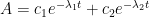
For the reversible, consecutive system, the following differential equations are:
The analytical solution to this system (apologies in advance if I made an algebra and/or transcription error) is given as follows:
where the two eigenvalues are:
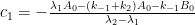
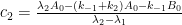
and the two coefficients are:
Here is a nice resource to look at:
http://voh.chem.ucla.edu/vohtar/spring05/classes/156/pdf/COMPLEX%20REACTIONS_2005_2.pdf
On pages 9 & 10, the author provides this system with an example of the biphasic kinetic plot. And on page 12, the author provides the complete solution assuming B0 = 0 and the second step is reversible.
Another nice resource is found here:
http://nova-transnet.com/zonanova/downloads/documentos/Basic%20Pharmacokinetics.pdf
The author provides concrete examples of how to use Laplace transforms to solve the compartment box models starting in section 2-44.
Ferdinand,
I would love to see your model. I’ve been trying to figure out how to do it putting formula windows in the NOAA or GFDL Carbon cycle graphics. Also very interested in how to approximate ocean chemistry from two or three of the variables.
gostapettersson says:
July 12, 2013 at 6:09 pm
A practically irreversible reaction by definition is characterized by k2 much smaller than k1, as the rate constants are defined by your formulas.
What you seems to refuse to understand is that both decay processes for 14C are (near) completely independent of each other. Thus k2 and k1 have not the slightest connection with each other. They simply work in parallel. Both are decay rates, not return rates (should have supplied them too as k-1 and k-2). k1 maybe much larger than k2 or reverse, in practice it is k2 which leads k1.
The general decay of all CO2 (all isotopes alike) is caused by pressure differences between atmosphere and oceans (both surface and deep oceans) and the biosphere. That is the first decay rate, which is bidirectional, but as the deep oceans are much larger in carbon content, in practice irreversible.
The specific decay for 14CO2 (and 13CO2) is caused by the concentration differences of what goes in and out other reservoirs. That is not much different for vegetation and the ocean’s surface, but is quite different for the deep oceans. That is the second decay rate, which is bidirectional, but as the deep oceans are much larger in carbon content, in practice irreversible. The second decay rate is only applicable to 14CO2 (and 13CO2), not to 12CO2.
Even if exactly the same quantities of total CO2 come back from the deep oceans as which did go in, what comes out as 14CO2 concentration is less than halve the concentration of what did go in at the peak of the bomb spike. Thus only halve the quantity of 14CO2 returns in the first year bomb spike than what did go in, while (near) exactly the same amount of 12CO2 returns (minus the negligible difference in 13CO2 and 14CO2 mass).
I am sorry to say that you have too much to learn about reaction kinetics already at the most elementary level
After 34 years practical experience with chemical processes by correcting theoretical models which didn’t work in reality (and 8 years of enjoyed retirement), I have forgotten most of the theoretical side, but still know where to look for the practical pitfalls of the theories…
ZP says:
July 12, 2013 at 6:34 pm
Should learn Latif, but have finished the process flows, I made two flowcharts with realistic figures for the years 1960:
http://www.ferdinand-engelbeen.be/klimaat/klim_img/14co2_distri_1960.jpg
and for 2000:
http://www.ferdinand-engelbeen.be/klimaat/klim_img/14co2_distri_2000.jpg
Here some more background (I hope that makes it clear):
The main process of redistribution of an excess CO2 injection is the same for all isotopes.
There are three main reservoirs where the excess CO2 can get into in reasonable time:
– vegetation
– ocean surface
– deep oceans.
The huge exchanges back and forth between air and vegetation/ocean surface and the limited uptake of both (10% of the change in the atmosphere for the ocean surface, 0.5% in vegetation) makes that the decay rates are quite fast (5 years according to the IPCC, 2 years to regain equilibrium of in/outflows).
The main process of redistribution of an excess 14CO2 follows the same rules as for all isotopes. Except that for the deep oceans there is an extra process at work: the concentration of what goes into the oceans largely differs from what comes out.
That is an (near) entirely separate process than the redistribution of all CO2 together. Thus to make the basis complete (where the = sign means the reversible reactions) for A (atmosphere), B (deep oceans), C(ocean surface) and D (biosphere):
A = B
A14 = B14
A = C
A14 = C14
A = D
A14 = D14
For simplicity, you may forget the ocean surface and vegetation out of the equations and simply add the redistribution to the deep oceans (where the bulk of the increase ultimately will reside). Both are fast in equilibrium for all isotopes and have little contribution to the mass decay. Over the period 1960-2000 the overall mass increase of vegetation was near zero
.
Thus for the current discussion forget all C&D reactions as well as for total CO2 as for 14CO2. What is left is the sink and source rates between atmosphere and deep oceans, for total CO2 and 14CO2.
Pre-bomb 14CO2 in the atmosphere and other reservoirs was ~50% of the bomb peak strength, more or less in equilibrium. Cosmic rays then supplied about 6% per year, which compensated for the losses in other reservoirs (mainly the oceans).
Thank you for the flowcharts. These diagrams make it clear that your model would predict a multiphasic decay profile for 14C from the atmosphere.
Ferdinand,
Very impressive flow charts.
ZP says:
July 13, 2013 at 5:35 am
These diagrams make it clear that your model would predict a multiphasic decay profile for 14C from the atmosphere.
As most of the distribution of the extra 14CO2 bomb releases into the ocean surface and the biosphere already occured before the peak value was reached and there is hardly any further decay in these reservoirs, I don’t see how that would be observable in the (relative) huge decay caused by the return of low 14C out of the deep oceans.
Thus my question is: what happens with 14CO2 compared to 12CO2 with the two decay rates involved for the deep oceans only: the in/out mass difference (for both) and the in/out concentration difference (for 14CO2 only)?
gymnosperm says:
July 13, 2013 at 10:43 am
Very impressive flow charts.
Thanks, the mass transfers are from GISS, but backcalculated for the 1960 data from the Mauna Loa curve and the known human emissions. The distribution in the ocean surface is based on the Revelle factor (for 12CO2 and 14CO2 alike). The distribution in the biosphere is from Battle e.a. where vegetation was a small net emitter before 1990 and a small, but increasing absorber after 1990.
The main uncertainty is the isotopic behaviour for vegetation and the ocean surface. At one side, when the concentration in the atmosphere drops (into the deep oceans), then the higher concentrations in vegetation and ocean surface will give some of it back to the atmosphere. On the other side, some of it drops out into the deep oceans (mainly as organics) or gets into more permanent land storage (humus, peat, browncoal,…).
So this are the basic isotopic schemes, open to improvements…
gymnosperm says:
July 13, 2013 at 10:43 am
“Very impressive flow charts.”
But, basically a balancing of the books according to a specific, and non-unique, scenario. I has no probative value.
It has no probative value.
Let’s ignore what happened before the peak value occurred as it won’t change the mathematical analysis. We can accurately analyze the implications of the proposed model without loss of information.


In short, you are showing three coupled equilibria as follows:
In this case, the observed time decay profile of 14C from the atmosphere levels will be dependent on the transfer rates into and out of each of the three sinks. So far, so good?
However, you appear to be asserting a critical mathematical constraint that equilibrium of the atmosphere with the surface and biosphere had been established by the time we started our analysis (i.e. at the peak value). If so, the rates into and out of those sinks must be equal by definition of equilibrium. Thus, the loss of A would be controlled only by the equilibration rate with the deep oceans.
However, this criterion is contrary to your flow diagram that appears to show the mass transfer rates into and out of the ocean surface and biosphere sinks as being unequal (i.e. there is a small net positive transfer into the sinks). Therefore, those systems are not at equilibrium (again by definition). The transfer rates into and out of a sink must be equal at all times in order for those sinks to be in equilibrium. If the sinks are not in equilibrium, then the model will predict a multiphasic kinetic profile for the loss of 14CO2 from the atmosphere. If the sinks are in equlibrium, then the model collapses to just:
which is indistinguishable from the model given by Gösta, albeit the interpretation of the parameters are slightly different.
ZP says:
July 13, 2013 at 1:52 pm
which is indistinguishable from the model given by Gösta, albeit the interpretation of the parameters are slightly different.
Except that the decay rates for 12CO2 (the bulk) and 14CO2 are widely different:
– in 1960, the mass loss of 12CO2 from the atmosphere into the deep oceans is:
(40-41) GtC/690 GtC = – 0.15%
– in 1960, the mass loss of 14CO2 from the atmosphere into the deep oceans is:
(( 40 GtC * 45% ) – (41 GtC * 100%)) / (690 GtC * 100%) = -3.33%
– in 2000, the mass loss of 12CO2 from the atmosphere into the deep oceans is:
(40-41.7) GtC/780 GtC = -0.22%
– in 2000, the mass loss of 14CO2 from the atmosphere into the deep oceans is:
(( 40 GtC * 45% ) – (41.7 GtC * 60%)) / (780 GtC * 60%) = -1.5%
In 1960, the 12CO2 level in the atmosphere was 17% above equilibrium
In 1960, the 14CO2 level in the atmosphere was 100% above equilibrium
In 2000, the 12CO2 level in the atmosphere was 28% above equilibrium
In 2000, the 14CO2 level in the atmosphere was 20% above equilibrium
For the same % above equilibrium, one should expect the same % mass loss, if a similar process with the same decay rate is at work.
In this case, different processes are at work: the decay of an excess amount 12CO2 in the atmosphere only depends on the difference between inputs and outputs (which is pessure dependent), while the decay rate of the 14CO2 bomb spike additionally depends on the bulk of the exchanges rates (which is temperature dependent) and the concentration differences between inputs and outputs.
Thus while the model is similar, the decay rate of 14CO2 is much faster than the decay rate of 12CO2, which represents near 99% of all CO2. And thus is the 14CO2 bomb spike curve not representative for the decay of an extra injection of CO2 above equilibrium.
It doesn’t matter. The predicted behavior is a direct consequence of the axioms of mathematics.
ZP says:
July 13, 2013 at 3:39 pm
It doesn’t matter. The predicted behavior is a direct consequence of the axioms of mathematics.
Agreed.
But the theory of Gösta Pettersson was:
the bombtest curve can be taken to be representative for the relaxation of emission pulses of carbon dioxide in general.
is proven false as different relaxation times are involved…
Bart says:
July 13, 2013 at 1:32 pm
But, basically a balancing of the books according to a specific, and non-unique, scenario. I has no probative value.
Besides balancing the books based on relative constant exchange rates between the different compartiments, the 14CO2 decay proves that there is no increase in exchange rates with the deep oceans over the period 1960-2000.
Human emissions increased a 2.8 fold 1960-2000.
If natural turnover is responsible for the atmospheric increase, the total natural inflows must have increased in ratio: from 180 GtC/year to 500 GtC/yr, assuming the estimates of 1960 as start.
As vegetation and ocean surface turnover are limited in variability, the deep oceans must take the difference, thus + 320 GtC/year turnover. That gives following flow estimates for the year 2000:
http://www.ferdinand-engelbeen.be/klimaat/klim_img/14co2_distri_2000_2.jpg
That doesn’t give a difference in net mass distribution, but it gives a huge difference in 14CO2 distribution:
With the extended deep ocean turnover in 2000, the mass loss of 14CO2 from the atmosphere into the deep oceans in one year then is:
(( 360 GtC * 45% ) – (361.7 GtC * 60%)) / (780 GtC * 60%) = -11.8%
Thus if there was such a real increase of natural deep ocean – atmosphere turnover, the year 2000 drop of 14CO2 from the bomb tests would be below the pre-bomb tests value, in only one year… Which isn’t observed.
The increase of deep ocean turnover thus is proven false (as good as it was from the 13CO2 decay rate).
This statement requires proof through calculation of the rate constants. Guesstimation of annual fluxes is not proof nor are assertions that the kinetic isotope effect will be unusually large for this system. At this time, I fail to see how your claim is defensible.
ZP says:
July 14, 2013 at 8:02 am
Guesstimation of annual fluxes is not proof nor are assertions that the kinetic isotope effect will be unusually large for this system.
The difference in rate constants is not caused by kinetic isotope effects, it is caused by a combination of sink rate (which is nearly the same for all isotopes) and the difference in concentration between 14C (or 13C) and 12C for what goes into the deep oceans and what comes out.
The observed relaxation time for an excess CO2 injection is 51.5 years.
The observed relaxation time for an excess 14CO2 injection is 14 years.
For 12C that is the effect of C – Ceq only.
For 14C that is the combined effect of C – Ceq ánd 14C – 14Caq.
Where the effect of the combination on 14C decay is much larger than the single effect on 12C.
Rate constants are independent of concentrations by definition. The rate of a non-zero-order process, however, is dependent on concentrations (as well as the rate constant).