
Studies of Carbon 14 in the atmosphere emitted by nuclear tests indicate that the Bern model used by the IPCC is inconsistent with virtually all reported experimental results.
Guest essay by Gösta Pettersson
The Keeling curve establishes that the atmospheric carbon dioxide level has shown a steady long-term increase since 1958. Proponents of the antropogenic global warming (AGW) hypothesis have attributed the increasing carbon dioxide level to human activities such as combustion of fossil fuels and land-use changes. Opponents of the AGW hypothesis have argued that this would require that the turnover time for atmospheric carbon dioxide is about 100 years, which is inconsistent with a multitude of experimental studies indicating that the turnover time is of the order of 10 years.
Since its constitution in 1988, the United Nation’s Intergovernmental Panel on Climate Change (IPCC) has disregarded the empirically determined turnover times, claiming that they lack bearing on the rate at which anthropogenic carbon dioxide emissions are removed from the atmosphere. Instead, the fourth IPCC assessment report argues that the removal of carbon dioxide emissions is adequately described by the ‘Bern model‘, a carbon cycle model designed by prominent climatologists at the Bern University. The Bern model is based on the presumption that the increasing levels of atmospheric carbon dioxide derive exclusively from anthropogenic emissions. Tuned to fit the Keeling curve, the model prescribes that the relaxation of an emission pulse of carbon dioxide is multiphasic with slow components reflecting slow transfer of carbon dioxide from the oceanic surface to the deep-sea regions. The problem is that empirical observations tell us an entirely different story.
The nuclear weapon tests in the early 1960s have initiated a scientifically ideal tracer experiment describing the kinetics of removal of an excess of airborne carbon dioxide. When the atmospheric bomb tests ceased in 1963, they had raised the air level of C14-carbon dioxide to almost twice its original background value. The relaxation of this pulse of excess C14-carbon dioxide has now been monitored for fifty years. Representative results providing direct experimental records of more than 95% of the relaxation process are shown in Fig.1.

Figure 1. Relaxation of the excess of airborne C14-carbon dioxide produced by atmospheric tests of nuclear weapons before the tests ceased in 1963
The IPCC has disregarded the bombtest data in Fig. 1 (which refer to the C14/C12 ratio), arguing that “an atmospheric perturbation in the isotopic ratio disappears much faster than the perturbation in the number of C14 atoms”. That argument cannot be followed and certainly is incorrect. Fig. 2 shows the data in Fig. 1 after rescaling and correction for the minor dilution effects caused by the increased atmospheric concentration of C12-carbon dioxide during the examined period of time.

Figure 2. The bombtest curve. Experimentally observed relaxation of C14-carbon dioxide (black) compared with model descriptions of the process.
The resulting series of experimental points (black data i Fig. 2) describes the disappearance of “the perturbation in the number of C14 atoms”, is almost indistinguishable from the data in Fig. 1, and will be referred to as the ‘bombtest curve’.
To draw attention to the bombtest curve and its important implications, I have made public a trilogy of strict reaction kinetic analyses addressing the controversial views expressed on the interpretation of the Keeling curve by proponents and opponents of the AGW hypothesis.
(Note: links to all three papers are below also)
Paper 1 in the trilogy clarifies that
a. The bombtest curve provides an empirical record of more than 95% of the relaxation of airborne C14-carbon dioxide. Since kinetic carbon isotope effects are small, the bombtest curve can be taken to be representative for the relaxation of emission pulses of carbon dioxide in general.
b. The relaxation process conforms to a monoexponential relationship (red curve in Fig. 2) and hence can be described in terms of a single relaxation time (turnover time). There is no kinetically valid reason to disregard reported experimental estimates (5–14 years) of this relaxation time.
c. The exponential character of the relaxation implies that the rate of removal of C14 has been proportional to the amount of C14. This means that the observed 95% of the relaxation process have been governed by the atmospheric concentration of C14-carbon dioxide according to the law of mass action, without any detectable contributions from slow oceanic events.
d. The Bern model prescriptions (blue curve in Fig. 2) are inconsistent with the observations that have been made, and gravely underestimate both the rate and the extent of removal of anthropogenic carbon dioxide emissions. On basis of the Bern model predictions, the IPCC states that it takes a few hundreds of years before the first 80% of anthropogenic carbon dioxide emissions are removed from the air. The bombtest curve shows that it takes less than 25 years.
Paper 2 in the trilogy uses the kinetic relationships derived from the bombtest curve to calculate how much the atmospheric carbon dioxide level has been affected by emissions of anthropogenic carbon dioxide since 1850. The results show that only half of the Keeling curve’s longterm trend towards increased carbon dioxide levels originates from anthropogenic emissions.
The Bern model and other carbon cycle models tuned to fit the Keeling curve are routinely used by climate modellers to obtain input estimates of future carbon dioxide levels for postulated emissions scenarios. Paper 2 shows that estimates thus obtained exaggerate man-made contributions to future carbon dioxide levels (and consequent global temperatures) by factors of 3–14 for representative emission scenarios and time periods extending to year 2100 or longer. For empirically supported parameter values, the climate model projections actually provide evidence that global warming due to emissions of fossil carbon dioxide will remain within acceptable limits.
Paper 3 in the trilogy draws attention to the fact that hot water holds less dissolved carbon dioxide than cold water. This means that global warming during the 2000th century by necessity has led to a thermal out-gassing of carbon dioxide from the hydrosphere. Using a kinetic air-ocean model, the strength of this thermal effect can be estimated by analysis of the temperature dependence of the multiannual fluctuations of the Keeling curve and be described in terms of the activation energy for the out-gassing process.
For the empirically estimated parameter values obtained according to Paper 1 and Paper 3, the model shows that thermal out-gassing and anthropogenic emissions have provided approximately equal contributions to the increasing carbon dioxide levels over the examined period 1850–2010. During the last two decades, contributions from thermal out-gassing have been almost 40% larger than those from anthropogenic emissions. This is illustrated by the model data in Fig. 3, which also indicate that the Keeling curve can be quantitatively accounted for in terms of the combined effects of thermal out-gassing and anthropogenic emissions.

Figure 3. Variation of the atmospheric carbon dioxide level, as indicated by empirical data (green) and by the model described in Paper 3 (red). Blue and black curves show the contributions provided by thermal out-gassing and emissions, respectively.
The results in Fig. 3 call for a drastic revision of the carbon cycle budget presented by the IPCC. In particular, the extensively discussed ‘missing sink’ (called ‘residual terrestrial sink´ in the fourth IPCC report) can be identified as the hydrosphere; the amount of emissions taken up by the oceans has been gravely underestimated by the IPCC due to neglect of thermal out-gassing. Furthermore, the strength of the thermal out-gassing effect places climate modellers in the delicate situation that they have to know what the future temperatures will be before they can predict them by consideration of the greenhouse effect caused by future carbon dioxide levels.
By supporting the Bern model and similar carbon cycle models, the IPCC and climate modellers have taken the stand that the Keeling curve can be presumed to reflect only anthropogenic carbon dioxide emissions. The results in Paper 1–3 show that this presumption is inconsistent with virtually all reported experimental results that have a direct bearing on the relaxation kinetics of atmospheric carbon dioxide. As long as climate modellers continue to disregard the available empirical information on thermal out-gassing and on the relaxation kinetics of airborne carbon dioxide, their model predictions will remain too biased to provide any inferences of significant scientific or political interest.
References:
Climate Change 2007: IPCC Working Group I: The Physical Science Basis section 10.4 – Changes Associated with Biogeochemical Feedbacks and Ocean Acidification
http://www.ipcc.ch/publications_and_data/ar4/wg1/en/ch10s10-4.html
Climate Change 2007: IPCC Working Group I: The Physical Science Basis section 2.10.2 Direct Global Warming Potentials
http://www.ipcc.ch/publications_and_data/ar4/wg1/en/ch2s2-10-2.html
GLOBAL BIOGEOCHEMICAL CYCLES, VOL. 15, NO. 4, PAGES 891–907, DECEMBER 2001 Joos et al. Global warming feedbacks on terrestrial carbon uptake under the Intergovernmental Panel on Climate Change (IPCC) emission scenarios
ftp://ftp.elet.polimi.it/users/Giorgio.Guariso/papers/joos01gbc[1]-1.pdf
Click below for a free download of the three papers referenced in the essay as PDF files.
Paper 1 Relaxation kinetics of atmospheric carbon dioxide
Paper 2 Anthropogenic contributions to the atmospheric content of carbon dioxide during the industrial era
Paper 3 Temperature effects on the atmospheric carbon dioxide level
================================================================
Gösta Pettersson is a retired professor in biochemistry at the University of Lund (Sweden) and a previous editor of the European Journal of Biochemistry as an expert on reaction kinetics and mathematical modelling. My scientific reasearch has focused on the fixation of carbon dioxide by plants, which has made me familiar with the carbon cycle research carried out by climatologists and others.
Phil. says:
July 9, 2013 at 9:53 am
I do not intend to waste any more time on you, Phil. You are so far out of your depth, it is just not worth the effort.
Bart says:
July 9, 2013 at 11:18 am
Phil. says:
July 9, 2013 at 9:53 am
I do not intend to waste any more time on you, Phil. You are so far out of your depth, it is just not worth the effort.
Bart you so tied up in your fake model and have no understanding of the underlying physics that I long ago gave up on your ever learning anything. The only reason for rebutting your nonsense is in case someone else here might think you know what you’re talking about. I suspect Ferdinand feels the same, other posters have said much the same, Steve Fitzpatrick for example.
You’ve not explained why this equation couldn’t equally explain the observations:
dCO2/dt = k*T + k1*CO2anthro +k2, just ran away and hid, as usual!
Phil. says:
July 9, 2013 at 12:47 pm
========================================
Yeah Phil, we’ve seen this before. Check out
http://wattsupwiththat.com/2013/01/20/analysis-shows-tidal-forcing-is-as-a-major-factor-in-enso-forcing/
and scroll to bottom. –AGF
I think the issue arises from the fact that Gösta is using formal kineticist’s terminology, while much of the climatology literature is written by scientists with (quite obviously) no formal training in kinetic analyses.
The simplistic waterbox model presented by Peter is identical to the kinetic model formulation presented by Gösta. The main difference is that Peter assumes three distinct decay periods. This assumption is inconsistent with the presented compartment box model and associated description, however. The more complex waterbox model can be summarized using the following reaction equations, where the reversible sinks (i.e. cycles) are combined into a single box to simplify the kinetic model:


irreversible addition processes:
reversible processes:
irreversible removal processes:
Let’s ignore the irreversible addition processes and accept the assumption that the remaining processes are governed by differential concentration levels. With these assumptions, the changes will be governed by the following system of differential equations:
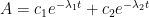
While an analytical solution to this system of differential equations exists, it is fairly involved, so an abbreviated solution describing the CO2 atmospheric levels (A) is given as follows:
Notice: this solution is of the same form as that given by the Bern model.
The two coefficients (c1 and c2) are functions of:
1) the initial concentrations of CO2 in the atmosphere
2) the initial concentrations of CO2 in the reversible sinks
3) the individual rate constants governing the transfers into and out of each compartment.
The two lambdas are formally referred to as eigenvalues of the coefficient matrix. The eigenvalues are just functions of the rate constants, the values of which exist in the complex plane – (i.e. the numerical values for the eigenvalues need not be real numbers).
Since the rate constants are functions of temperature, the coefficients and eigenvalues will also be functions of temperature. However, only the rate constants obey the Arrhenius equation, so the coefficients and eigenvalues will vary in highly complex ways with changes in temperature. And, if the temperature changes with time, one cannot solve the system of differential equations analytically. The only option is to solve the system numerically.
Hopefully, this form will parse correctly:
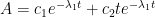
if the eigenvalues are not repeating:
otherwise:
Phil. says:
July 9, 2013 at 12:47 pm
“You’ve not explained why this equation couldn’t equally explain the observations”
Did, too.
Let us know when you’ve completed your first course in high school algebra. Then, maybe you can interact constructively.
agfosterjr says:
July 9, 2013 at 2:59 pm
Great. Tweedle-dee to the rescue of Tweedle-dum.
Gene Selkov says:
July 9, 2013 at 3:32 pm
Ah, another anti-Einstein crackpot. This thread has definitely jumped the shark.
Greg: “…comes close to reconciling Gosta Pettersson’s C14 curve and the Bern model”
Dear Greg, please be patient. I hope to be able to address other parts of your comments tomorrow, but today I will restrict myself to a simple technical question: The mathematical description of the bombtest curve.
As pointed out by Wallace you get a better fit the more exponential terms you add to your regression function. Ten exponential terms fit the curve better than a monoexponential function, but the fit is not much better. The descriptive rule you have to consider in such a case is to use the simplest function giving a satisfactory fit, i.e. a fit that is not improved with statistical significance when you add an extra exponential term. The decision as to the adequate number of terms to use can be made by standard statistical methods. Such tests formed the basis for my conclusions in Paper 1 that a monoexponential function provides a satisfactory fit and that no statistically significant improvement of fit was obtained for a biexponential function. Wallace seems to favour this view, as does the RMSE values he provides.
So, from a statistical point of view, the bombtest curve is best described as monoexponential. Otherwise, I wouldn’t mind a bit using Wallace’s biexponential function as an impulse response functionin my calculations. This would just confirm my conclusion that emissions only account for one half of the increased air level of CO2.
But I disagree with your statement that this reconciles the C14 curve and the Bern model. Relaxation times of the exponential terms in Wallace’s function seem to agree satisfactorily with those of the first two terms of the Bern model, but the amplitudes do not. Wallace’s function describes the observations made, the Bern model does not. Wallace’s function provides the same inferences as my monoexponential function, the Bern model provides entirely different inferences.
The reason for that is that the designers of model started by postulating what the inferences should be and then tuned parameter values in the model to be consistent with that postulate rather than with the observations made.
Bart says:
July 9, 2013 at 6:53 pm
Phil. says:
July 9, 2013 at 12:47 pm
“You’ve not explained why this equation couldn’t equally explain the observations”
Did, too.
No you didn’t come close to addressing it there.
Let us know when you’ve completed your first course in high school algebra. Then, maybe you can interact constructively.
Before you were born kid!
I do interact constructively, you on the other hand just get abusive with anyone who points out your lack of knowledge of the physics and doesn’t accept your bogus equation.
Ferdinand E.: “The main problem with the Pettersson 14C bomb spike is the dilution of 14C by the deep ocean and other reservoirs”
Phil: “14C diluted by CO2 from fossil fuel combustion, … also the oceans from which CO2 returns is depleted in 14C”
Greg: ” some correction to the C14 curve is required before the fitting”
Dilution effects on reported 14CO2/12CO2 ratios are approximately equal to (actually about 1% lower than) those indicated by the increased air level of CO2 during the examined periods of time; only an increase of atmospheric 12CO2 can dilute the atmospheric 14CO2/12CO2 ratio, and does so irrespective of whether the increase derives from fossil fuel combustion, return of 14C-free CO2 from the oceans, thermal outgassing, vulcanism or other sources.
Data in Fig. 2 of my Paper 1 have been corrected by consideration of the increased CO2 level (with the assumption that it exclusively derives from 12CO2). The correction, therefore, has taken care of all the dilution effects you discuss.
No additional corrections are required, unless you wish to correct the corrections for the fact that only 99% of the increase is 12CO2, the rest 13CO2. But such a sophisticated level of correction of the corrections is uncalled for because the corrections have a minor effect on the overall shape of the curve (the largest correction factor ≈1.2 applies for the latest point and raises its value from observed ≈4% to ≈5% in the corrected plot). The is borne out by my and Wallace’s regression analyses of the uncorrected data, which provide the same time constant estimate (≈14 years) as obtained for the corrected data.
gostapettersson says:
July 10, 2013 at 9:00 am
No additional corrections are required
Indeed, you did correct for the increase of CO2 in the atmosphere by the 14C free human emissions. But that is by far not the largest necessary correction.
The largest influence on 14CO2 levels is by the exchanges with the deep oceans: that is about 5% of all CO2 in the atmosphere which is replaced by deep ocean CO2. That doesn’t change the 12C levels of the atmosphere, but it does change the 14C level: what goes in the deep oceans is the current 14C/12C ratio, what comes out is the 14C/12C ratio of ~1000 years ago, minus the decay of 14C over that time frame.
Thus the problem is that you didn’t take into account the extra reduction of the 14C levels caused by the exchange with the deep oceans with 14C levels which are 55% lower than the peak bomb test values.
That gives the largest part of the 14 years relaxation time, not the redistribution of the extra CO2 in the atmosphere.
That makes that the relaxation time for the 14C spike is over 3 times faster than for the extra 12/13CO2 spike. And that you can’t assume that the 14C spike decay represents the fate of the extra CO2 spike…
Some addition:
only an increase of atmospheric 12CO2 can dilute the atmospheric 14CO2/12CO2 ratio
No, the exchange with the deep oceans doesn’t increase the 12CO2 mass in the atmosphere. It is only swapping amounts: the total amount of CO2 going in and out is near equal. But there is huge difference in 14C/12C ratio of what goes into the deep oceans and what comes out of the oceans. There is some 1000 years lag between sink and source. Thus anyway, what comes out the oceans is pre-bomb tests and what goes into the oceans is post-bomb tests…
Bart says:
> Ah, another anti-Einstein crackpot. This thread has definitely jumped the shark.
Heh. Those of us who are anti-nonsense don’t care about its origins. We don’t care if it comes from Einstein, Newton, our bosses, our girlfriends, or ourselves. When we see nonsense, we’re anti-everybody. No special treatment for you or your heroes — you’ll be greeted with the same crackpot attitude.
Ferdinand,


All physico-chemical processes are reversible. However, some processes are so slow as to be essentially irreversible. With that, you appear to be claiming that the reversibility of a 12CO2 molecule is substantially different from a 14CO2 molecule. If so (and quite frankly), the statement is incredible.
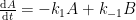
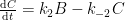
I’m assuming the the kinetic model that you are employing is best represented as follows (where A represents the atmospheric concentrations, B represents the upper ocean concentrations, and C represents the concentrations in the deep oceans).
(If this is incorrect, please provide the compartment box model – and associated system of differential equations – that you are assuming adequately describes the exchange process.)
This compartment box model will be governed by the following system of differential equations:
Your apparent assertion requires at least one of the following to be true:
1)
2)
3)
4)
Cases 1 and 3 are both inconsistent with known kinetic isotope effects; rate constants for heavier isotopes will be smaller than those of lighter isotopes. Thus, we can readily rule these two cases out. Cases 2 and 4 are also unlikely; the rate constants for 12CO2 should be a maximum of 5% larger than that for 14CO2.
Furthermore, the data provided by Gösta shows no apparent biphasic kinetic behavior implying that the loss of 14C follows (an/a set of parallel) irreversible pathway(s) or a single reversible pathway. The analysis by Gösta suggests the latter.
As the apparent claim is inconsistent with standard kinetic analyses, perhaps you have the data (or an alternative model) to support it. The required data would be the oceanic 14C concentrations as a function of time over the same time-frame as analyzed by Gösta. If plausible, we would expect the concentrations in the upper ocean layers to grow with time before decaying as the 14C flows into the deep ocean layers. The 14C concentrations in the deep ocean should grow slowly with time, followed by a more rapid growth and finishing with a slow growth rate. If you do not have these data, then Gösta’s analysis is significantly more plausible and consistent with standard kinetic analyses which invoke Occam’s razor.
Phil: “C14 decay curve isn’t representative of CO2 because it’s the result of a different set of
sources and sinks. C14 is created in the atmosphere from nitrogen”
Sources and sinks are of no primary interest as concerns representativity. Anthropogenic CO2 emissions come from many different sources, and sinks for 14CO2 and anthropogenic CO2 are the same (the hydrosphere and the biosphere).
The 14CO2 spike was created from nitrogen by the bomb tests, but once created it decays by the same reactions and mechanisms as CO2 in general. The C14 decay curve is representative of CO2 fro the simple reason that 14CO2 is carbon dioxide and carbon isotope effects are of negligible magnitude.
Assuming the systems response to C12 is the same as it is to C14, we can model the behaviour using control theory. We already know the Step Response (from the bomb tests).
ZP says:
July 10, 2013 at 5:35 pm
With that, you appear to be claiming that the reversibility of a 12CO2 molecule is substantially different from a 14CO2 molecule
Not at all: for the decay of any excess CO2 in the atmosphere, 12CO2 and 14CO2 follows the same rules, besides some small differentiation from isotope kinetics.
But for exchanges with the deep oceans, there is (near) zero decay for 12C, but a huge decay rate for 14C due to differences in 14C/12C ratio between what is in the atmosphere and what returns from the oceans.
I’m assuming the the kinetic model that you are employing is best represented as follows
In general it is simpler, as the deep ocean exchanges largely bypass the ocean surface, as well as at the sink places (mainly NE Atlantic) as at the source places (mainly near the Chilean coast).
If plausible, we would expect the concentrations in the upper ocean layers to grow with time before decaying as the 14C flows into the deep ocean layers.
See: http://shadow.eas.gatech.edu/~kcobb/isochem/lectures/lecture10_14C.ppt
From sheet 13 on, the 14C bomb spike in the oceans is covered.
Of particular interest is sheet 17, where the 14C spike (of +1000 per mil in the atmosphere) is largely suppressed at the Galapagos islands, due to the nearby deep ocean upwelling near the Chilean coast.
The deep ocean exchanges don’t influence the 12CO2 levels in the atmosphere, except for the difference between the inputs an outputs (which for the deep oceans currently is estimated at 2 GtC/year). But it does influence the 14C/12C ratio, even if there was no difference between inputs and outputs, as what comes in has a (much) lower 14C/12C ratio than the ratio in the atmosphere.
That makes that the decay rate of the 14C/12C ratio quite differs from the excess CO2 decay rate in general.
For excess CO2 decay (all isotopes) the formula is:
dCO2/dt = -k1*(C – Ceq)
where C is the current CO2 level (~400 ppmv) in the atmosphere and Ceq the equilibrium CO2 level for the current temperature (~290 ppmv).
Specific for 14CO2 the formula is:
dCO2/dt = -k1*(C14 – C14eq) – k2*(C14 – C14aq)
Where C14 is the current 14CO2 level in the atmosphere, C14eq the equilibrium 14CO2 level at the current temperature (quite similar to the general CO2 decay) and C14aq the 14CO2 level which returns from the deep oceans.
In this case k2 >> k1. The 14CO2 bomb spike relaxation is mainly by thinning of the concentration by deep ocean exchanges, not from the excess CO2 decay.
justjoshin says:
July 10, 2013 at 7:19 pm
Assuming the systems response to C12 is the same as it is to C14, we can model the behaviour using control theory. We already know the Step Response (from the bomb tests).
See my response to ZP: the system response to 14C is the same as for 12C for mass transfer, but additionally 14C is also removed by concentration differences between what returns from the deep oceans and what is present in the atmosphere…
gostapettersson says:
July 10, 2013 at 6:13 pm
The C14 decay curve is representative of CO2 fro the simple reason that 14CO2 is carbon dioxide and carbon isotope effects are of negligible magnitude.
That is true for the mass transfers which in general are the same for all isotopes, but for 14CO2 there is an extra concentration transfer which isn’t present for 12CO2 and which is much larger than for the mass transfers. Thus the 14C decay curve is not representative for the CO2 mass transfers…
gostapettersson says:
July 10, 2013 at 6:13 pm
Phil: “C14 decay curve isn’t representative of CO2 because it’s the result of a different set of
sources and sinks. C14 is created in the atmosphere from nitrogen”
Sources and sinks are of no primary interest as concerns representativity. Anthropogenic CO2 emissions come from many different sources, and sinks for 14CO2 and anthropogenic CO2 are the same (the hydrosphere and the biosphere).
The 14CO2 spike was created from nitrogen by the bomb tests, but once created it decays by the same reactions and mechanisms as CO2 in general. The C14 decay curve is representative of CO2 fro the simple reason that 14CO2 is carbon dioxide and carbon isotope effects are of negligible magnitude.
No they aren’t since the CO2 at the ocean surface is order 1,000 years old which doesn’t effect C12 but certainly does deplete the C14 returning from the ocean surface.
The equation that you have provided does not support your description. The equation you provided states that 14C will reversibly pass directly into the deep ocean without any exchange with the surface waters. And, will also reversibly exchange between the surface and atmosphere. So, the suggested model is correctly described by the following compartment box model:

As before A represents the atmospheric concentrations, B is the fast, reversible equilibrium (your C14eq term) and C represents the the deep ocean (your C14aq) term.
The solution to this system will again be consistent with the Bern Model with two terms. As stated previously, the solution will have two eigenvalues, the values of which will be functions of the rate constants.
Unless the equilibration with the biosphere is virtually instantaneous, this model would predict biphasic kinetics for the atmospheric 14C concentrations. This is not observed in the data.
Thanks for the data, but it does not provide justification for employing an mathematical model that is not founded in the language of formal kinetics. I strongly recommend that you revisit your thinking on this subject. Draw out the process using compartment boxes to represent the various sources and sinks. Draw arrows (reversible or not) from each source to each sink. From this diagram, write out the formal differential equations describing the process. Decide if a solution exists and solve the system either analytically or numerically, as applicable.
ZP says:
July 11, 2013 at 6:18 am
Ferdinand Engelbeen says:
July 11, 2013 at 3:15 am
In general it is simpler, as the deep ocean exchanges largely bypass the ocean surface, as well as at the sink places (mainly NE Atlantic) as at the source places (mainly near the Chilean coast).
Specific for 14CO2 the formula is:
dCO2/dt = -k1*(C14 – C14eq) – k2*(C14 – C14aq)
Where C14 is the current 14CO2 level in the atmosphere, C14eq
The equation that you have provided does not support your description. The equation you provided states that 14C will reversibly pass directly into the deep ocean without any exchange with the surface waters. And, will also reversibly exchange between the surface and atmosphere. So, the suggested model is correctly described by the following compartment box model:
No that isn’t a correct model, you have omitted the irreversible decay in reservoir C!
ZP says:
July 11, 2013 at 6:18 am
The equation you provided states that 14C will reversibly pass directly into the deep ocean without any exchange with the surface waters.
The deep ocean exchanges indeed largely bypass the surface, but are virtually non-reversable, as what returns from the deep oceans is what was going down some 1000 years ago. Thus the excess 14C in the atmosphere will be gone long before some of it returns from the deep oceans, and even that effect will be diluted, as smeared with a long period (several hundred years) filter. The C14aq in practice may be used as a constant.
The removal of total CO2 (including 14CO2) in excess as mass is quite fast distributed over ocean surface and vegetation with relaxation times of around 1 year, thus near instantaneous, but limited in quantity (10% of the change in the atmosphere for ocean surface). The more permanent storage in vegetation and deep oceans is what takes much more time.
Further, the 14C dilution is the result of two quite different processes: the general process of removal of an excess amount of CO2, which is mainly pressure (difference) related and the specific process of 14C concentrations changes by deep ocean exchanges which is mainly temperature (difference) related. These processes are virtually independent of each other and simply work in parallel.
As the exchange with the deep oceans is about a factor 20 larger than the removal rate of the excess amount of CO2 (all isotopes) into the deep oceans, it is no wonder that the excess removal rate has hardly any effect on the decay rate of 14CO2. Even the inclusion or exclusion of the thinning of 14C by the use of 14C-free fossil fuels at twice the excess removal rate had little effect (less than 1%) on the decay rate of 14CO2.
That may or may not match the different terms of the Bern model, but that is not the base of my reasoning. The base is that the empirical findings show a relaxation time for 14CO2 of ~14 years, while the relaxation time for the extra CO2 injection is ~52 years, over three times slower.
Similar as for the relaxation time of the 13CO2 depleted CO2 from fossil fuel burning: 3 times faster for 13CO2 than for the bulk of CO2, thanks to the deep ocean exchanges:
http://www.ferdinand-engelbeen.be/klimaat/klim_img/deep_ocean_air_zero.jpg
But if you want, I can try to make a multi-box model with all exchanges on it…
Phil. says:
July 11, 2013 at 6:45 am
No that isn’t a correct model, you have omitted the irreversible decay in reservoir C!
Look at it again. Irreversible decay is simply governed by the magnitude of k2 as compared to k-2. All processes are reversible in accordance with the principle of microscopic reversibility. However, some processes take a long time to reverse due to differences in magnitudes of the rate constants.
Clarification, some processes appear to be irreversible due to large differences in the magnitudes of the rate constants.
ZP says:
July 11, 2013 at 8:29 am
Phil. says:
July 11, 2013 at 6:45 am
No that isn’t a correct model, you have omitted the irreversible decay in reservoir C!
Look at it again. Irreversible decay is simply governed by the magnitude of k2 as compared to k-2. All processes are reversible in accordance with the principle of microscopic reversibility. However, some processes take a long time to reverse due to differences in magnitudes of the rate constants.
No, that refers to rate of transfer to and from the deep, during the ~1,000 years the C14 spends in the deep it decays to N14, that is not a reversible process! In fact by measuring the C14 at the ocean surface is how we know that the surface water is ~1,000 years old. You can find the data at: http://radiocarbon.pa.qub.ac.uk/marine/
Rather than show the deep water interaction as a reversible reaction you should show it as three sequential reactions, the C14 that returns from the deep has decayed, your model doesn’t include that.