
Studies of Carbon 14 in the atmosphere emitted by nuclear tests indicate that the Bern model used by the IPCC is inconsistent with virtually all reported experimental results.
Guest essay by Gösta Pettersson
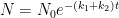
The Keeling curve establishes that the atmospheric carbon dioxide level has shown a steady long-term increase since 1958. Proponents of the antropogenic global warming (AGW) hypothesis have attributed the increasing carbon dioxide level to human activities such as combustion of fossil fuels and land-use changes. Opponents of the AGW hypothesis have argued that this would require that the turnover time for atmospheric carbon dioxide is about 100 years, which is inconsistent with a multitude of experimental studies indicating that the turnover time is of the order of 10 years.
Since its constitution in 1988, the United Nation’s Intergovernmental Panel on Climate Change (IPCC) has disregarded the empirically determined turnover times, claiming that they lack bearing on the rate at which anthropogenic carbon dioxide emissions are removed from the atmosphere. Instead, the fourth IPCC assessment report argues that the removal of carbon dioxide emissions is adequately described by the ‘Bern model‘, a carbon cycle model designed by prominent climatologists at the Bern University. The Bern model is based on the presumption that the increasing levels of atmospheric carbon dioxide derive exclusively from anthropogenic emissions. Tuned to fit the Keeling curve, the model prescribes that the relaxation of an emission pulse of carbon dioxide is multiphasic with slow components reflecting slow transfer of carbon dioxide from the oceanic surface to the deep-sea regions. The problem is that empirical observations tell us an entirely different story.
The nuclear weapon tests in the early 1960s have initiated a scientifically ideal tracer experiment describing the kinetics of removal of an excess of airborne carbon dioxide. When the atmospheric bomb tests ceased in 1963, they had raised the air level of C14-carbon dioxide to almost twice its original background value. The relaxation of this pulse of excess C14-carbon dioxide has now been monitored for fifty years. Representative results providing direct experimental records of more than 95% of the relaxation process are shown in Fig.1.

Figure 1. Relaxation of the excess of airborne C14-carbon dioxide produced by atmospheric tests of nuclear weapons before the tests ceased in 1963
The IPCC has disregarded the bombtest data in Fig. 1 (which refer to the C14/C12 ratio), arguing that “an atmospheric perturbation in the isotopic ratio disappears much faster than the perturbation in the number of C14 atoms”. That argument cannot be followed and certainly is incorrect. Fig. 2 shows the data in Fig. 1 after rescaling and correction for the minor dilution effects caused by the increased atmospheric concentration of C12-carbon dioxide during the examined period of time.

Figure 2. The bombtest curve. Experimentally observed relaxation of C14-carbon dioxide (black) compared with model descriptions of the process.
The resulting series of experimental points (black data i Fig. 2) describes the disappearance of “the perturbation in the number of C14 atoms”, is almost indistinguishable from the data in Fig. 1, and will be referred to as the ‘bombtest curve’.
To draw attention to the bombtest curve and its important implications, I have made public a trilogy of strict reaction kinetic analyses addressing the controversial views expressed on the interpretation of the Keeling curve by proponents and opponents of the AGW hypothesis.
(Note: links to all three papers are below also)
Paper 1 in the trilogy clarifies that
a. The bombtest curve provides an empirical record of more than 95% of the relaxation of airborne C14-carbon dioxide. Since kinetic carbon isotope effects are small, the bombtest curve can be taken to be representative for the relaxation of emission pulses of carbon dioxide in general.
b. The relaxation process conforms to a monoexponential relationship (red curve in Fig. 2) and hence can be described in terms of a single relaxation time (turnover time). There is no kinetically valid reason to disregard reported experimental estimates (5–14 years) of this relaxation time.
c. The exponential character of the relaxation implies that the rate of removal of C14 has been proportional to the amount of C14. This means that the observed 95% of the relaxation process have been governed by the atmospheric concentration of C14-carbon dioxide according to the law of mass action, without any detectable contributions from slow oceanic events.
d. The Bern model prescriptions (blue curve in Fig. 2) are inconsistent with the observations that have been made, and gravely underestimate both the rate and the extent of removal of anthropogenic carbon dioxide emissions. On basis of the Bern model predictions, the IPCC states that it takes a few hundreds of years before the first 80% of anthropogenic carbon dioxide emissions are removed from the air. The bombtest curve shows that it takes less than 25 years.
Paper 2 in the trilogy uses the kinetic relationships derived from the bombtest curve to calculate how much the atmospheric carbon dioxide level has been affected by emissions of anthropogenic carbon dioxide since 1850. The results show that only half of the Keeling curve’s longterm trend towards increased carbon dioxide levels originates from anthropogenic emissions.
The Bern model and other carbon cycle models tuned to fit the Keeling curve are routinely used by climate modellers to obtain input estimates of future carbon dioxide levels for postulated emissions scenarios. Paper 2 shows that estimates thus obtained exaggerate man-made contributions to future carbon dioxide levels (and consequent global temperatures) by factors of 3–14 for representative emission scenarios and time periods extending to year 2100 or longer. For empirically supported parameter values, the climate model projections actually provide evidence that global warming due to emissions of fossil carbon dioxide will remain within acceptable limits.
Paper 3 in the trilogy draws attention to the fact that hot water holds less dissolved carbon dioxide than cold water. This means that global warming during the 2000th century by necessity has led to a thermal out-gassing of carbon dioxide from the hydrosphere. Using a kinetic air-ocean model, the strength of this thermal effect can be estimated by analysis of the temperature dependence of the multiannual fluctuations of the Keeling curve and be described in terms of the activation energy for the out-gassing process.
For the empirically estimated parameter values obtained according to Paper 1 and Paper 3, the model shows that thermal out-gassing and anthropogenic emissions have provided approximately equal contributions to the increasing carbon dioxide levels over the examined period 1850–2010. During the last two decades, contributions from thermal out-gassing have been almost 40% larger than those from anthropogenic emissions. This is illustrated by the model data in Fig. 3, which also indicate that the Keeling curve can be quantitatively accounted for in terms of the combined effects of thermal out-gassing and anthropogenic emissions.

Figure 3. Variation of the atmospheric carbon dioxide level, as indicated by empirical data (green) and by the model described in Paper 3 (red). Blue and black curves show the contributions provided by thermal out-gassing and emissions, respectively.
The results in Fig. 3 call for a drastic revision of the carbon cycle budget presented by the IPCC. In particular, the extensively discussed ‘missing sink’ (called ‘residual terrestrial sink´ in the fourth IPCC report) can be identified as the hydrosphere; the amount of emissions taken up by the oceans has been gravely underestimated by the IPCC due to neglect of thermal out-gassing. Furthermore, the strength of the thermal out-gassing effect places climate modellers in the delicate situation that they have to know what the future temperatures will be before they can predict them by consideration of the greenhouse effect caused by future carbon dioxide levels.
By supporting the Bern model and similar carbon cycle models, the IPCC and climate modellers have taken the stand that the Keeling curve can be presumed to reflect only anthropogenic carbon dioxide emissions. The results in Paper 1–3 show that this presumption is inconsistent with virtually all reported experimental results that have a direct bearing on the relaxation kinetics of atmospheric carbon dioxide. As long as climate modellers continue to disregard the available empirical information on thermal out-gassing and on the relaxation kinetics of airborne carbon dioxide, their model predictions will remain too biased to provide any inferences of significant scientific or political interest.
References:
Climate Change 2007: IPCC Working Group I: The Physical Science Basis section 10.4 – Changes Associated with Biogeochemical Feedbacks and Ocean Acidification
http://www.ipcc.ch/publications_and_data/ar4/wg1/en/ch10s10-4.html
Climate Change 2007: IPCC Working Group I: The Physical Science Basis section 2.10.2 Direct Global Warming Potentials
http://www.ipcc.ch/publications_and_data/ar4/wg1/en/ch2s2-10-2.html
GLOBAL BIOGEOCHEMICAL CYCLES, VOL. 15, NO. 4, PAGES 891–907, DECEMBER 2001 Joos et al. Global warming feedbacks on terrestrial carbon uptake under the Intergovernmental Panel on Climate Change (IPCC) emission scenarios
ftp://ftp.elet.polimi.it/users/Giorgio.Guariso/papers/joos01gbc[1]-1.pdf
Click below for a free download of the three papers referenced in the essay as PDF files.
Paper 1 Relaxation kinetics of atmospheric carbon dioxide
Paper 2 Anthropogenic contributions to the atmospheric content of carbon dioxide during the industrial era
Paper 3 Temperature effects on the atmospheric carbon dioxide level
================================================================
Gösta Pettersson is a retired professor in biochemistry at the University of Lund (Sweden) and a previous editor of the European Journal of Biochemistry as an expert on reaction kinetics and mathematical modelling. My scientific reasearch has focused on the fixation of carbon dioxide by plants, which has made me familiar with the carbon cycle research carried out by climatologists and others.
gostapettersson says:
July 7, 2013 at 6:55 pm
In addition to my previous message of July 8, 2013 at 11:40 am, where I calculated the 14C “dilution” decay by the deep oceans as slightly over 18 years, the calculated decay rate from excess CO2 decay may be added as:
1/Tau14C = 1/Taudeepdilute + 1/TauCO2plus
1/Tau14C = 1/18.19 + 1/51.2
That gives Tau14C = 13.4 years
Et voila, the decay rate of the 14C bomb spike fully explained by the mix of deep ocean thinning and excess CO2 distribution over different reservoirs…
Ferdinand proposed:
> 1/Tau14C = 1/Taudeepdilute + 1/TauCO2plus
>
> 1/Tau14C = 1/18.19 + 1/51.2
>
> That gives Tau14C = 13.4 years
But does that give us a process that can match the observed data? I presume your model of the mix is a sum of two exponential decay processes defined by the two time constants. If that is so, it is not possible to fit any linear combination of exp(-t/18.19) and exp(-t/51.2) to the data modelled with exp(-t/13.4). If it is not a sum, then what is it?
Greg Goodman says:
July 8, 2013 at 12:06 pm
Now since you are obviously quite unwilling to learn anything here and I’ve explained it a least ten times, I have better things to do than to try in vain to explain to one Engelbeen how this should be done.
Greg, I am a bit slower than in the past, but what you tried to explain simply makes no sense:
– some decay is over halve a year and the other halve there is no decay.
– the same total decay is spread over the full year.
That gives that in both cases the decay rate is the same over a full year (the same amount is removed…)and there is no difference in e-folding time over several years. You simply didn’t take into account the halve year that there was zero decay, thus an infinite decay rate (try to add these two decay rates together…).
But besides this point, what do you think of my calculation of the combination of the 14C dilution by deep ocean exchanges and the excess CO2 decay time?
Ferdinand Engelbeen says:
July 8, 2013 at 1:08 pm
try to add these two decay rates together…
Which is quite simple as the second term aproaches zero… But the first term is wrong, as one need to take the average decay over a year, not what happens over halve a year.
Bart says:
July 8, 2013 at 9:53 am
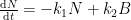
This argument would be so much easier if certain people understood calculus. The evidence is very clear. CO2 in the atmosphere evolves according to the equation
dCO2/dt = k*(T – Teq)
Although your data appears to show the following relationship:
dCO2/dt = 0.205*(HADCRUT4SH anomaly) + 0.1
Any particular reason to choose the Southern Hemisphere?
Also that anomaly is relative to the mean from 1961-1990, why would you expect that to represent Teq?
Of course if it wasn’t for the offset term (that you omitted) the fact that the temperature term was negative until 1978 would have your equation yielding a reduction in CO2 not the observed increase!
Gene Selkov says:
July 8, 2013 at 12:05 pm
“Mathematics has never been the language of science.”
Since the days of the Enlightenment, yes it has.
“It has no independent validity and it is not incorruptible; on the contrary, it is often used to cover up bad ideas.”
Name one. Mathematics itself cannot be corrupted, though people can fail adequately to understand it and arrive at false conclusions. It is the language of nature itself, in the measure of quantities, fields, and fluxes, bound by a set of rigid rules which cannot be abrogated.
Ferdinand Engelbeen says:
July 8, 2013 at 12:00 pm
“If you don’t accept any data which doesn’t fit your hypothesis, then we are end of discussion.”
It is you who are not accepting the data which does not fit your hypothesis, not I. You do not have anything compelling. I do. Your dCO2 ratios and the like are open to many interpretations. The derivative relationship is not.
“All you have is a nice fit, caused by a completely arbitrary baseline.”
The baseline is arbitrary in any case. The temperature data themselves are with respect to an arbitrary baseline. It is inherent in the problem.
But, it does not help you, because the emissions data are not ambiguous to within an arbitrary baseline offset. There is a definite trend in them. But, that trend is already accounted for in the temperature relationship, and it is not arbitrary. So, you cannot willy-nilly substitute in your trend from the emissions and remove the trend from the temperature relationship. Nature has no mechanism for performing this feat. It is entirely a mental construct on your part, which is not grounded in reality.
“If one and only one observation is violated, then the hypothesis is rejected.”
There are no violations of the hypothesis that Nature is overwhelmingly responsible for observed CO2 levels. Your evidences are mere interpretations to construct a narrative. But, they are not compelling. Just because you have a scenario which you imagine to be consistent with the observations does not elevate that scenario to a fundamental observation itself.
Your interpretation runs completely afoul of the observed relationship
dCO2/dt = k*(T – Teq)
There is no physically possible way to reconcile that observation with significant human forcing of atmospheric CO2.
“What is the effect of more CO2 on dCO2/dt.”
Negligible. That is what the relationship above shows.
“Does the circulation of CO2 increase in ratio with the human emissions and how affects that the residence time.”
The full system is one in which atmospheric CO2 tracks the natural level being pumped into the atmosphere by the temperature relationship. It is analogous to the following coupled system, which I discussed previously:
dCO2_pumped/dt = k*(T – Teq)
dCO2_total/dt = ( CO2_pumped – CO2_total)/tau + H
The e-folding time in this analogous system is tau. In the real world, the true response may have multiple time scales. But, those time scales should generally be more or less constant and independent of the the inputs. The rate of change of CO2_total is affected by H, the rate of human emissions, but the effect is relatively small. Assuming tau is relatively short, the solution of the differential equation is approximately
CO2_total := CO2_pumped + tau*H
As tau approaches zero, so does the effect of H on the overall concentration. This refers back to the discussion of the “mass balance” argument, and how it depends entirely on the efficiency of the sinks. A short tau means the sinks are very efficient, and so the influence of H becomes negligible, and CO2_total approaches CO2_pumped.
Bart says:
> Gene Selkov says:
> July 8, 2013 at 12:05 pm
>
>> “It has no independent validity and it is not incorruptible; on the contrary, it is often used to cover up bad ideas.”
>
> Name one.
Ric = 0
Can name plenty more, but we are far off-topic already.
> Mathematics itself cannot be corrupted, though people can fail adequately to understand it and arrive at false conclusions.
This is why it is so helpful in driving people to false conclusions. It is the only thinking mode I am aware about that is subject to cancer-like growth, for its own sake. Good for you if you can manage it and if it serves a purpose. If you can solve real problems with it, you are my hero. But when you start pushing mathematical explanations of nature, don’t expect any cheers.
> It is the language of nature itself, in the measure of quantities, fields, and fluxes, bound by a set of rigid rules which cannot be abrogated.
So it was nature itself that whispered a bunch of tensor expressions conveying the idea of a single-mass universe (or otherwise empty universe) to Einstein and his mathematician buddies? And now no day passes by that I don’t hear crap about black holes and big bang, and such. My children suffered from it at school. It’s on the telly all the time and it has infected the pop culture. And you want to tell me it’s not corruption, or that mathematics had nothing to do with it?
Rigid rules which cannot be abrogated? Watch a replay of how they were, early in the Enlightenment:
http://milesmathis.com/calcor.html
Gene Selkov says:
July 8, 2013 at 1:34 pm
But does that give us a process that can match the observed data? I presume your model of the mix is a sum of two exponential decay processes defined by the two time constants.
Yes it is the sum of the two time constants. But that gives a new time constant for the combined processes, even if these are completely unrelated. If that matches the observed data? I presume yes, to a certain extent, as the empirical data give a similar time constant for the decay.
As my math is very rusty, I borrowed the combined decay rate formula from:
http://citizendia.org/Exponential_decay#Decay_by_two_or_more_processes
Which shows that the sum of two decay rates is easely converted into one new single decay rate.
Of course there still are (minor) difficulties to solve: the 14C ratio decline is also influenced by the thinning from 14C-free combustion of fossil fuels (which is corrected for by Pettersson, but not by me), but on the other side, there is a constant supply of fresh 14C from cosmic rays…
Ferdinand says:
> As my math is very rusty, I borrowed the combined decay rate formula from:
> http://citizendia.org/Exponential_decay#Decay_by_two_or_more_processes
> Which shows that the sum of two decay rates is easely converted into one new single decay rate.
Now I get it, thank you. It is like discharging a capacitor through a pair of resistors connected in parallel, which is no different than discharging the same capacitor through a single resistor representing the harmonic mean of the two.
Phil. says:
July 8, 2013 at 1:52 pm
“Although your data appears to show the following relationship:
dCO2/dt = 0.205*(HADCRUT4SH anomaly) + 0.1”
Which is
dCO2/dt = 0.205*(HADCRUT4SH_anomaly – (-0.1/0.205)) = 0.205*(HADCRUT4SH_anomaly – 0.4878)
so, Teq for the Southern hemisphere data is Teq = -0.1/0.205 = -0.4878 := -0.5 degC.
“Any particular reason to choose the Southern Hemisphere?”
It appears to fit better, and that supports the hypothesis that this is largely an oceanic phenomenon.
“Also that anomaly is relative to the mean from 1961-1990, why would you expect that to represent Teq?”
Teq is relative to the dataset being used. If Southern hemispheric temperatures prepared and presented as here were to drop by 0.5 degC, we should see the CO2 increase level off. Stay tuned, it may happen in the next several years.
“Of course if it wasn’t for the offset term (that you omitted) the fact that the temperature term was negative until 1978 would have your equation yielding a reduction in CO2 not the observed increase!”
As you see from above, I did not omit it, I simply had it in a different order in the equation.
But, this is key. The only thing needed for a match here is the offset in temperature due to Teq. If human emissions were a constant, then I could not say with any assurance that the baseline so computed were not at least partially due to human inputs.
But, human inputs have not been constant. They have had a distinct and significant trend. There is no room for additional trend in the relationship – it is already accounted for by the temperature sensitivity. Hence, we must conclude that human inputs have insignificant influence.
Bart says:
July 8, 2013 at 2:30 pm
dCO2/dt = k*(T – Teq)
There is no physically possible way to reconcile that observation with significant human forcing of atmospheric CO2.
Except that the k*(T-Teq) is completely spurious for the longer term change and thus only is a mathematical fit of the curve, not an “observation”. While my own fit is less good for the short term variability, the fit for the longer term upswing is better than yours:
http://www.ferdinand-engelbeen.be/klimaat/klim_img/co2_T_dT_em_1960_2005.jpg
especially going back in time:
http://www.ferdinand-engelbeen.be/klimaat/klim_img/co2_T_dT_em_1900_2005.jpg
Thus human forcing is as good (even better) than temperature for fitting the long-term trend. I only need to improve the temperature driven short term variability.
“What is the effect of more CO2 on dCO2/dt.”
Negligible. That is what the relationship above shows.
That is circular reasoning and it violates the physics involved.
If CO2 in the atmosphere increases, the pressure difference between oceans and atmosphere at the warm side decreases and the outflux decreases in ratio with the pressure difference decrease. The opposite happens at the cold side of the oceans. That gives a reduction of the increase rate in the atmosphere which over time gets to zero. That is completely neglected in your formula.
CO2_total := CO2_pumped + tau*H
As tau approaches zero, so does the effect of H on the overall concentration. This refers back to the discussion of the “mass balance” argument, and how it depends entirely on the efficiency of the sinks.
Besides that H is not negligible, as the average residence time gives about 150 GtC for CO_pumped, there is a measurable increase of 70 ppmv over the past 50 years in the atmosphere, mimicking the overall trend of the CO2 emissions, which more than doubled over that time frame. That means that the CO2_pumped also should have more than doubled over the same time period. Thus reducing the residence time to less than halve. Of which is not the slightest indication…
Ferdinand Engelbeen says:
July 8, 2013 at 3:17 pm
“While my own fit is less good for the short term variabilit…”
That means your “fit” does not fit. All you are doing is matching up a 1st order trend. That is always easy to do. What’s hard is matching up all across the frequency spectrum, both the short and the long term. When you do that, you find you have no need for the emissions data at all to explain the entire record.
“That is circular reasoning and it violates the physics involved.”
No circular reasoning. There simply is no such effect evident in the data.
“That gives a reduction of the increase rate in the atmosphere which over time gets to zero.”
No, it does not. You are still stuck in a static analysis.
“Besides that H is not negligible…”
The effect is tau * H. As tau goes to zero, that product goes to zero, too.
“That means that the CO2_pumped also should have more than doubled over the same time period.”
It’s just a steady accumulation of the CO2 being pumped into the atmosphere from the ocean dynamics.
“…especially going back in time…”
For various reasons, projecting back in time is problematic, owing to significantly lower quality data, and lack of direct observation of the dynamics, which can vary with time.
It is a moot question. It does not matter.
Over the last 55 years, the rate of change of CO2 has been an affine function of temperature, and emissions have not influenced it significantly. That is all one needs to know.
One thing that might be causing confusion is if you think CO2_pumped is an actual quantity of CO2 being pumped into the atmosphere. But, I could have written the equations as
dP/dt = k1*(T – Teq)
dCO2_total/dt = –CO2_total/tau + H + P
Here, P is the rate at which CO2 is being pumped into the system. In terms of my previous nomenclature, P = CO2_pumped/tau and k1 = k/tau. CO2_pumped is the “instantaneous equilibrium level” of CO2 resulting from the action of P, but P is the actual induced rate of change of CO2. It is being forced in by the upwelling of CO2 rich waters in such quantity that it is overwhelming the ability of the sinks to keep it down.
The action of the term –CO2_total/tau represents sink activity, as well as offsetting pressure such as you are looking for, or any other mechanism which resists the rise due to the ocean pumping.
Bart says:
July 8, 2013 at 2:44 pm
Phil. says:
July 8, 2013 at 1:52 pm
“Although your data appears to show the following relationship:
dCO2/dt = 0.205*(HADCRUT4SH anomaly) + 0.1″
Which is
dCO2/dt = 0.205*(HADCRUT4SH_anomaly – (-0.1/0.205)) = 0.205*(HADCRUT4SH_anomaly – (-0.4878))
Just noticed I left off the minus sign, which might cause confusion.
It is important to show the compartment box model if you are going to perform these calculations. This calculation assumes two parallel, irreversible processes:


 latex N\rightleftharpoons B$

Described by the following differential equation:
having the following analytical solution:
This solution is not equivalent to a sum of exponentials of the form:
and is described by a system of differential equations of the form:
It is important to show the compartment box model if you are going to perform these calculations. This calculation assumes two parallel, irreversible processes:


Giving the following differential equation:
with the following analytical solution:
This solution is not equivalent to a sum of exponentials of the form:
consistent with the form given by the Bern Model.
Nor is it consistent with the compartment box model suggested by Gösta, which has the form:
yielding a system of differential equations of the form:
gymnosperm: “How good a proxy is 14CO2 for the other isotopes?”
My Paper 1 page 7 gives you a clue: “Carbon isotope effects encountered in
organic chemistry may occasionally be as high as 1.15 [16], but are normally much lower [17].
The kinetic isotope effects for events associated with the uptake of atmospheric carbon dioxide by
the hydrosphere or the biosphere have been extensively studied and are normally lower than 1.02 for C13 and 1.04 for C14 [18, 19].”
This means that the isotope effects are of negligible magnitude compared to the experimental error in data such as the bombtest curve. 14CO2 is an excellent proxy for CO2 in general and anthropogenic CO2 emissions in particular.
Dear Ferdinand Engelbeen,
Please forgive for saying so, but your meager knowledge of relaxation kinetics makes your comments so full of unjustified or erroneous statements that I had better confine myself to a few fundamental points that may help you understand why I disagree with most of your views on such topics.
1. F.E.: “residence time is how much CO2 is exchanged”
You accept the standard definition of residence/turnover time (used by the IPCC, used by me). What you may not realize is that this definition is a reformulation of the law of mass action; residence time is the reciprocal of the rate constant for a specified unidirectional output step and not a measure of exchange. Rate constants are system constants. Doubling the amount of CO2 does not change the corresponding residence time. All that happens is that the corresponding output rate is doubled.
And the “decay time” for 14CO2 is NOT a residence time. You seem to be the one of us who has a poor understanding of the difference between the two “time” concepts, i.e. the difference between rate constants and relaxation time constants (which are functions of the rate constants).
2. Almost all carbon cycle models are of multibox character and based on prescriptions of the law of mass action. The standard approach is to define the system by detailing the number of boxes considered, their interconnections, and the rate constants characterizing the exchange of carbon between the boxes. The law of mass action is then applied to express the relaxation kinetics (the pulse response) of the system in terms of differential equations such as d[CO2air]/dt = f(concentration variables; rate constants). To the extent that the equations have an analytical solution, they may prescribe that relaxations of concentration variables in the system are governed by exponential relationships. The solutions then also show how the corresponding relaxation times are related to rate constants in the system.
So, when you claim that a quantity “tau = Expression” represents the “excess mass decay rate” for CO2 emissions, you have to provide evidence for that claim. Define your system, show that the kinetic equations can be solved, show that the solution corresponds to exponential relaxation terms, and show that the relaxation time for CO2 is adequately described by your “Expression”. The latter seems unlikely, because relaxation times are functions of rate constants in the system and your “Expression” shows no obvious relationship to any rate constants at all.
3. F. E.: “Besides (negligibly small isotope effects), all carbon isotopes behave the same”
I agree, and the implication of your statement is that reaction schemes, rate constants, and the kinetic differential equations for all carbon isotopes are practically the same. Which means that solutions to the equations, and hence relaxation times, are practically the same for 14CO2 and emissions of fossil CO2. The possibility that the 14CO2 spike and emissions of fossil CO2 decay at widely different rates does not exist. Your claim that the latter relaxation time is 52.5 years is unsupported by tenable evidence and inconsistent with the relaxation time of 14 years empirically estimated for 14CO2 from the bombtest curve.
Bart says:
July 8, 2013 at 2:30 pm
Your interpretation runs completely afoul of the observed relationship
dCO2/dt = k*(T – Teq)
That is not the observed relationship, the observed relationship in your data fitting is:
dCO2/dt = k*T + offset
You assume that there is a Teq which is given by k*offset, you have no evidence for this.
There is no physically possible way to reconcile that observation with significant human forcing of atmospheric CO2.
Yes there is:
dCO2/dt = k*T + k1*CO2anthro +k2, where CO2anthro is the rate of human release of CO2.
“What is the effect of more CO2 on dCO2/dt.”
Negligible. That is what the relationship above shows.
No that’s a result of your assumption!
gostapetterson,
“The kinetic isotope effects for events associated with the uptake of atmospheric carbon dioxide by
the hydrosphere or the biosphere have been extensively studied and are normally lower than 1.02 for C13 and 1.04 for C14 [18, 19].”
Your source [19] is paywalled but I quote from [18]: “If stomatal diffusion is rapid (stomatal resistance is low) and carboxylation is limiting, the predicted isotope fractionation is 28%…If diffusion is slow (stomatal resistance is high), the predicted fracrionation is 4%…”
He is talking about C4 plants and C3 are a bit more efficient under dry (high resistance) conditions, but ocean biota don’t have this problem at all and moist tropical areas not so much.
Overall I would bet biological fractionation is closer to 1.1 than 1.02 for 13C and higher for 14C. I think you should give some serious consideration to heavy isotope concentration in the oceans where DIC just doesn’t care and 1/5 of the carbon cycle disappears every year into the abyss for a millennium.
Bart says:
July 8, 2013 at 3:46 pm
No circular reasoning. There simply is no such effect evident in the data.
Bart, if your formula (that is not data!) shows something that violates physics, then your formula is wrong.
If the CO2 pressure in the atmosphere increases, then the overall increase of CO2 into the atmosphere is decreased. Whatever the cause of the increase. That is independent of the type of process involved, as good for a static process as for a dynamic changing process.
ZP says:
July 8, 2013 at 7:09 pm
Thanks for the comment…
In my opinion, indeed the two processes involved are quasy independent of each other and both are practically irreversable.
The Bern model has its problems, and may be justified if you add most of all known reserves of oil and gas (at 3000 GtC) plus coal (at 5000 Gtc) to the atmosphere. Then several of the current fast sinks become saturated and even a “constant” fraction may be the case. Not with the up to current releases, which may give a 1% remaining fraction if all CO2 released equilibrates with the deep oceans (after several centuries).
Pettersson’s approach is that only the distribution of CO2 over the different reservoirs plays a role and doesn’t take into account the thinning caused by the deep oceans difference in 14C content.
In my opinion, both are wrong…
gostapettersson says:
July 8, 2013 at 8:29 pm
OK, I have some difficulties with the different (English) definitions, where several quite different ones are mangled for the same prcess and the same are used for quite different processes.
The possibility that the 14CO2 spike and emissions of fossil CO2 decay at widely different rates does not exist. Your claim that the latter relaxation time is 52.5 years is unsupported by tenable evidence and inconsistent with the relaxation time of 14 years empirically estimated for 14CO2 from the bombtest curve.
Again, what you forget is that the 14CO2 decay rate is heavily influenced by the “thinning” caused by the huge exchanges with deep ocean waters. What goes into the deep oceans is the current atmospheric composition, what comes out is the atmospheric composition of ~1000 years ago, minus the 14C decay rate. Anyway (far) lower than the post-bomb tests 14C level, 55% lower than the initial bomb spike.
That has nothing to do with the relaxation of any excess injection of CO2 in the atmosphere, which is more or less the same for all isotopes (except for the isotopic discrimination). That gives that the decay rate for 14C is much faster than for 12C.
The same happens for 13CO2:
http://www.ferdinand-engelbeen.be/klimaat/klim_img/deep_ocean_air_zero.jpg
Where only 1/3rd of the theoretical decay of 13C of the fossil fuel injection is found. Thus compared to the relaxation time of the extra CO2 injection, the relaxation of 13C vs. 12C is three times faster.
The 52.5 relaxation time is as empirical as your 14C relaxation time: based on real world changes in total atmospheric CO2 (as mass) vs. the extra pressure caused by the extra CO2 increase above the pre-industrial equilibrium. See the same explanation as mine by Dr. Peter Dietze in 1997:
http://www.john-daly.com/carbon.htm
It is a simple two box model where the extra amount (=pressure) invokes an extra outflow from one box (the atmosphere) into one other reservoir (representing all other reservoirs combined). Currently the extra outflow is 4-5 GtC/year for a level of 210 GtC (100 ppmv) above equilibrium, giving a relaxation time of over 50 years for the extra CO2 (all isotopes combined). Over 3 times slower than for 14C. Not by coincidence a similar upspeed as for 13C.
Phil. says:
July 8, 2013 at 9:02 pm
“You assume that there is a Teq which is given by k*offset, you have no evidence for this.”
Holy cow. Are you really this dense? I’ve tried to spoon feed it to you, but this is basic algebra. If you cannot understand it, give up. You have no hope of understanding anything about this system.
Ferdinand Engelbeen says:
July 9, 2013 at 12:08 am
“Bart, if your formula (that is not data!) shows something that violates physics, then your formula is wrong.”
No, it simply means that the effect is minor, and can be neglected. If you read through the comment above, you will see that I explain why.
Ferdinand Engelbeen says:
July 9, 2013 at 1:18 am
“What goes into the deep oceans is the current atmospheric composition, what comes out is the atmospheric composition of ~1000 years ago, minus the 14C decay rate.”
Just for the record, I agree with you here, and this is a singularly lucid explanation. There are undoubtedly several time constants involved, though the data indicate that those active in sequestering anthropogenic inputs are short.
It is also a window into the ocean pump. What was the composition of 1000 years ago? And, if it was much higher than today, how does that upwelling of higher content waters affect CO2 concentrations today? Answer: it produces a continuous pump into the atmosphere, which will not stop until the temperature/pressure/concentration states reach a new equilibrium.
Bart says:
July 9, 2013 at 9:11 am
Phil. says:
July 8, 2013 at 9:02 pm
“You assume that there is a Teq which is given by k*offset, you have no evidence for this.”
Holy cow. Are you really this dense? I’ve tried to spoon feed it to you, but this is basic algebra. If you cannot understand it, give up. You have no hope of understanding anything about this system.
It is clear that you don’t understand the system at all. You have asserted that the only explanation for the offset is Teq, however you have never attempted to justify this. Then in a classical case of circular reasoning you then assert that that means there is no role for human CO2 release! As I pointed out there could be other terms in that offset which you have not accounted for, including human CO2 release, which you blithely ignore. Explain why the offset must be completely accounted for by the Teq term and what evidence you rely on in that assertion. Mathematics without the proper physics/physical chemistry is meaningless!
ZP says:
July 8, 2013 at 7:14 pm
The actual set of ordinary differential equations is a truncated expansion in eigenmodes of the solution to a partial differential diffusion equation. They are generally a convenient fiction – until added together, they do not necessarily model actual, specific and discrete physical processes.
Each eigenstate has a specific time constant associated with it. When you add all the responses together, you get something like the Bern Model.
So, the problem with the Bern Model is not the methodology. It is that it has been fitted based on presumed dynamics which, it has now become evident, are wrong.