
Studies of Carbon 14 in the atmosphere emitted by nuclear tests indicate that the Bern model used by the IPCC is inconsistent with virtually all reported experimental results.
Guest essay by Gösta Pettersson
The Keeling curve establishes that the atmospheric carbon dioxide level has shown a steady long-term increase since 1958. Proponents of the antropogenic global warming (AGW) hypothesis have attributed the increasing carbon dioxide level to human activities such as combustion of fossil fuels and land-use changes. Opponents of the AGW hypothesis have argued that this would require that the turnover time for atmospheric carbon dioxide is about 100 years, which is inconsistent with a multitude of experimental studies indicating that the turnover time is of the order of 10 years.
Since its constitution in 1988, the United Nation’s Intergovernmental Panel on Climate Change (IPCC) has disregarded the empirically determined turnover times, claiming that they lack bearing on the rate at which anthropogenic carbon dioxide emissions are removed from the atmosphere. Instead, the fourth IPCC assessment report argues that the removal of carbon dioxide emissions is adequately described by the ‘Bern model‘, a carbon cycle model designed by prominent climatologists at the Bern University. The Bern model is based on the presumption that the increasing levels of atmospheric carbon dioxide derive exclusively from anthropogenic emissions. Tuned to fit the Keeling curve, the model prescribes that the relaxation of an emission pulse of carbon dioxide is multiphasic with slow components reflecting slow transfer of carbon dioxide from the oceanic surface to the deep-sea regions. The problem is that empirical observations tell us an entirely different story.
The nuclear weapon tests in the early 1960s have initiated a scientifically ideal tracer experiment describing the kinetics of removal of an excess of airborne carbon dioxide. When the atmospheric bomb tests ceased in 1963, they had raised the air level of C14-carbon dioxide to almost twice its original background value. The relaxation of this pulse of excess C14-carbon dioxide has now been monitored for fifty years. Representative results providing direct experimental records of more than 95% of the relaxation process are shown in Fig.1.

Figure 1. Relaxation of the excess of airborne C14-carbon dioxide produced by atmospheric tests of nuclear weapons before the tests ceased in 1963
The IPCC has disregarded the bombtest data in Fig. 1 (which refer to the C14/C12 ratio), arguing that “an atmospheric perturbation in the isotopic ratio disappears much faster than the perturbation in the number of C14 atoms”. That argument cannot be followed and certainly is incorrect. Fig. 2 shows the data in Fig. 1 after rescaling and correction for the minor dilution effects caused by the increased atmospheric concentration of C12-carbon dioxide during the examined period of time.

Figure 2. The bombtest curve. Experimentally observed relaxation of C14-carbon dioxide (black) compared with model descriptions of the process.
The resulting series of experimental points (black data i Fig. 2) describes the disappearance of “the perturbation in the number of C14 atoms”, is almost indistinguishable from the data in Fig. 1, and will be referred to as the ‘bombtest curve’.
To draw attention to the bombtest curve and its important implications, I have made public a trilogy of strict reaction kinetic analyses addressing the controversial views expressed on the interpretation of the Keeling curve by proponents and opponents of the AGW hypothesis.
(Note: links to all three papers are below also)
Paper 1 in the trilogy clarifies that
a. The bombtest curve provides an empirical record of more than 95% of the relaxation of airborne C14-carbon dioxide. Since kinetic carbon isotope effects are small, the bombtest curve can be taken to be representative for the relaxation of emission pulses of carbon dioxide in general.
b. The relaxation process conforms to a monoexponential relationship (red curve in Fig. 2) and hence can be described in terms of a single relaxation time (turnover time). There is no kinetically valid reason to disregard reported experimental estimates (5–14 years) of this relaxation time.
c. The exponential character of the relaxation implies that the rate of removal of C14 has been proportional to the amount of C14. This means that the observed 95% of the relaxation process have been governed by the atmospheric concentration of C14-carbon dioxide according to the law of mass action, without any detectable contributions from slow oceanic events.
d. The Bern model prescriptions (blue curve in Fig. 2) are inconsistent with the observations that have been made, and gravely underestimate both the rate and the extent of removal of anthropogenic carbon dioxide emissions. On basis of the Bern model predictions, the IPCC states that it takes a few hundreds of years before the first 80% of anthropogenic carbon dioxide emissions are removed from the air. The bombtest curve shows that it takes less than 25 years.
Paper 2 in the trilogy uses the kinetic relationships derived from the bombtest curve to calculate how much the atmospheric carbon dioxide level has been affected by emissions of anthropogenic carbon dioxide since 1850. The results show that only half of the Keeling curve’s longterm trend towards increased carbon dioxide levels originates from anthropogenic emissions.
The Bern model and other carbon cycle models tuned to fit the Keeling curve are routinely used by climate modellers to obtain input estimates of future carbon dioxide levels for postulated emissions scenarios. Paper 2 shows that estimates thus obtained exaggerate man-made contributions to future carbon dioxide levels (and consequent global temperatures) by factors of 3–14 for representative emission scenarios and time periods extending to year 2100 or longer. For empirically supported parameter values, the climate model projections actually provide evidence that global warming due to emissions of fossil carbon dioxide will remain within acceptable limits.
Paper 3 in the trilogy draws attention to the fact that hot water holds less dissolved carbon dioxide than cold water. This means that global warming during the 2000th century by necessity has led to a thermal out-gassing of carbon dioxide from the hydrosphere. Using a kinetic air-ocean model, the strength of this thermal effect can be estimated by analysis of the temperature dependence of the multiannual fluctuations of the Keeling curve and be described in terms of the activation energy for the out-gassing process.
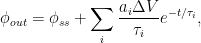
For the empirically estimated parameter values obtained according to Paper 1 and Paper 3, the model shows that thermal out-gassing and anthropogenic emissions have provided approximately equal contributions to the increasing carbon dioxide levels over the examined period 1850–2010. During the last two decades, contributions from thermal out-gassing have been almost 40% larger than those from anthropogenic emissions. This is illustrated by the model data in Fig. 3, which also indicate that the Keeling curve can be quantitatively accounted for in terms of the combined effects of thermal out-gassing and anthropogenic emissions.

Figure 3. Variation of the atmospheric carbon dioxide level, as indicated by empirical data (green) and by the model described in Paper 3 (red). Blue and black curves show the contributions provided by thermal out-gassing and emissions, respectively.
The results in Fig. 3 call for a drastic revision of the carbon cycle budget presented by the IPCC. In particular, the extensively discussed ‘missing sink’ (called ‘residual terrestrial sink´ in the fourth IPCC report) can be identified as the hydrosphere; the amount of emissions taken up by the oceans has been gravely underestimated by the IPCC due to neglect of thermal out-gassing. Furthermore, the strength of the thermal out-gassing effect places climate modellers in the delicate situation that they have to know what the future temperatures will be before they can predict them by consideration of the greenhouse effect caused by future carbon dioxide levels.
By supporting the Bern model and similar carbon cycle models, the IPCC and climate modellers have taken the stand that the Keeling curve can be presumed to reflect only anthropogenic carbon dioxide emissions. The results in Paper 1–3 show that this presumption is inconsistent with virtually all reported experimental results that have a direct bearing on the relaxation kinetics of atmospheric carbon dioxide. As long as climate modellers continue to disregard the available empirical information on thermal out-gassing and on the relaxation kinetics of airborne carbon dioxide, their model predictions will remain too biased to provide any inferences of significant scientific or political interest.
References:
Climate Change 2007: IPCC Working Group I: The Physical Science Basis section 10.4 – Changes Associated with Biogeochemical Feedbacks and Ocean Acidification
http://www.ipcc.ch/publications_and_data/ar4/wg1/en/ch10s10-4.html
Climate Change 2007: IPCC Working Group I: The Physical Science Basis section 2.10.2 Direct Global Warming Potentials
http://www.ipcc.ch/publications_and_data/ar4/wg1/en/ch2s2-10-2.html
GLOBAL BIOGEOCHEMICAL CYCLES, VOL. 15, NO. 4, PAGES 891–907, DECEMBER 2001 Joos et al. Global warming feedbacks on terrestrial carbon uptake under the Intergovernmental Panel on Climate Change (IPCC) emission scenarios
ftp://ftp.elet.polimi.it/users/Giorgio.Guariso/papers/joos01gbc[1]-1.pdf
Click below for a free download of the three papers referenced in the essay as PDF files.
Paper 1 Relaxation kinetics of atmospheric carbon dioxide
Paper 2 Anthropogenic contributions to the atmospheric content of carbon dioxide during the industrial era
Paper 3 Temperature effects on the atmospheric carbon dioxide level
================================================================
Gösta Pettersson is a retired professor in biochemistry at the University of Lund (Sweden) and a previous editor of the European Journal of Biochemistry as an expert on reaction kinetics and mathematical modelling. My scientific reasearch has focused on the fixation of carbon dioxide by plants, which has made me familiar with the carbon cycle research carried out by climatologists and others.
Have a look at 2005, the colour mapping is “cooler” and the hot spots stand out nicely. Moscow , New York and China. Nuff said?
TerryS: molecules are flowing into and out of the atmosphere at equal rates
  to keep the CO
 in the atmosphere at a level
  . Under this regime
  of the molecules that were in the atmosphere at time
  remain at time
  : the mean residence time is
  .
. of CO
of CO instantaneously at time
  . We assume that the added concentration causes
  to change to


 s and
s and  s demonstrates what the folks meant above by saying that the residence time is a different animal from the Bern-formula time constants. If
  ,
,  , and
, and  , the mean steady-state residence time is 10, changing after the
  disturbance only a little, to between 9.7 and 10.4 according to the Bern formula. But, if
  is 5 instead of 1 to make the mean steady-state residence time 2 instead of 10, the Bern formula yields a residence time between 2.03 and 2.14–with the same time constants.
Although your initial comment seemed compelling at first, I have now been able to explain to myself what the folks above meant when they said that the residence time is a different animal from the Bern formula time constants. Just in case it helps any other layman out there who had the same difficulty I did, I’ll set forth what I think they meant.
Suppose that at steady state CO
But let’s change the scenario and add a slug
where
so that the CO$_{2}$ amount obeys the Bern formula:
Now, instead of a constant average residence time $V_{ss} /\phi_{ss}$, the residence-time average changes with time:
Putting numbers to those equations with the Bern numbers for the
Nick Stokes says:
And as to endless claims that all the new CO2 in the air has nothing to do with us – I’m sure Ferdinand Engelbeen will once again try to convey some sense on that. But the basic question – we’ve burnt about 400 Gt Carbon, and put it in the air. There is about 200 Gt more there than there used to be. If it isn’t ours, but came from the sea or wherever, then where did ours go?
This seems to confirm that it doesn’t stick around very long. If it’s true that we’ve emitted 400 Gt(the bulk of that in more recent years) and only increased the amount by 200 Gt.
” If it isn’t ours, but came from the sea or wherever, then where did ours go?”
Into the ocean and biosphere. Some of molecules that went into the ocean came out again to satisfy the outgassing. It’s assumed to be a linear system so you just work separately and add the results.
If there was no temperature rise, all but the last few percent of emissions eventually get absorbed, on the same basis as the C14 curve. If SST rises without any GHG emissions, whatever out-gassing required to restore equilibrium will happen. The net result is a linear superposition of the two effects.
I had this same discussion a few days ago elsewhere and someone said “it can’t be a sink and a source, you have to choose”.
Well, as explained it can. The net result is a linear superposition of the two effects.
BTW , I did a deconvolution of MLO with the 14y exponential and just looks a little rougher, nothing like the emissions data. I also did it with 2.6 (the shortest part of Bern model) and it got a bit rougher still … and looked even less like emissions.
” While they are remotely connected, the turnover of capital/goods says next to nothing about the gain or loss of that bussiness.”
Ferdinand, we love you, but this betrays a lack of business experience. The Carbon cycle has a huge (200gt) volume and it is a very profitable business. It feeds the biosphere. It is the World Bank for Carbon cash flow.
Couple things barely touched on; 14C is the heaviest and least likely isotope to be biologically absorbed. This should mean that it has the LONGEST residence time in the atmosphere. The oceans are supersaturated with 13 and 14C because these isotopes are biologically rejected both on land and preferentially washed in and in the oceans themselves where there is vast and unquantified biological activity
Ocean down welling uptake will vary with atmospheric isotopic composition at the edge of the ice near the poles. Upwelling outgassing along mid latitude and subtropical continental margins and along the ITC in the open oceans will return that isotopic signal to the atmosphere nearly a millennium later.
In a weird economic sense the isotopic skew of outgassing acts like the control of interest rates by the Federal Reserve. Spewing 12C is quantitative easing. Spewing 14C is like 18% interest.
mike g says: July 2, 2013 at 8:31 pm
“This seems to confirm that it doesn’t stick around very long. If it’s true that we’ve emitted 400 Gt(the bulk of that in more recent years) and only increased the amount by 200 Gt.”
This is described as the airborne fraction. As emissions have risen, it works out that about half of each increment appears to go into the ocean, half stays in the air. Of course, this is total net change. This is in a period of steady rise; whar would happen if the rise slowed hasn’t really been tested.
Joe Born says:
July 2, 2013 at 8:29 pm
But let’s change the scenario and add a slug of CO2 instantaneously at time …… etc etc …….
———————————————–
Do we know of any planets where that actually happens ?
“Bart says:
July 2, 2013 at 4:45 pm”
I agree with that assessment of Ferdinand’s confusion.
Tried to tell him something similar ages ago but it didn’t sink in.
There seems to be a general assumption that the mechanism for CO2 outgassing from the oceans is symmetric to the mechanism of CO2 being absorbed into the oceans. This assumtion implicitely means that this process only happens at the surface of the oceans, but is it really that simple?
Outgassing from the oceans is clearly a function of the temperature of the ocean and the CO2 concentration in the atmosphere and possibly to some extent a function of wind speed which increases/decreases the effective water surface area.
Absorption of CO2 back into the oceans is clearly symmetric to outgassing on the simplest level. On the other hand there are probably an additional and probably fairly important additional mechanism for extracting CO2 out of the atmosphere (I intentionally leave the biosphere out). It seems obvious to me that rain is a very efficient CO2 pump extracting CO2 from air. Why? The surface area of water drops in for example a thunder storm is extremely high and this is combined with a fairly long residence time of water drops at temperatures close to freezing even in tropical areas (dT=30K or more).
Does anybody have any interesting links to airplane measurements of CO2 inside rain clouds? I think the expected CO2 concentrations should be clearly lower than in the bulk of the atmosphere.
Are there measurements of CO2 concentration at surface levels in warm/cold areas of the earth? I expect the CO2 concentration should increase in tropical areas close to the surface during/after a thunder storm because CO2 was extracted from higher layers of the atmosphere and deposited on the ground where at least parts of the CO2 is released when the water heats up.
In cold areas the effect is probably weaker and a larger proportion of the CO2 ends up back in the ocean.
They can, because they measure different things. That is what all the objections to this posting are about. The 17 is the amount of CO2 molecules left from the pulse. The 73 is the excess of water.
I see that you have a good working analogy with your bucket with four chambers. Your model behaves as the formula, good job, but so do another with mixed gases which I will describe below:
Imagine a leaky bucket under an open tap. The bucket has four holes, one in the bottom and three just above the equilibrium level. The stream from the tap represents the natural CO2 sources and is constant. The leakage from the hole in the bottom represents natural sinks and is equal the natural sources.
All the dynamics caused by pouring a pulse of extra water in the bucket is explained by the three holes just above the equilibrium level. That means that the leakage from hole in the bottom in this model is independent of the water level.
I remind again of the Bern formula:
Each of the holes is connected to a closed tank on the outside of the bucket. The tank connected to the big hole representing lifetime of 1.186 years fill up after 18,6% of the pulse has drained.
The tank connected to the medium hole representing lifetime of 18.51 years fill up after 33.8% of the pulse has drained.
The tank connected to the smallest hole representing lifetime of 172.9 years fill up after 25.9% of the pulse has drained.
Observe that while this is going on the leakage from the hole in the bottom and the pouring from the tap, continues as before. That is the reason that the amount of molecules from the pulse is down to 17% after 5 years, but the amount of excess water is 73% of the pulse.
So to your objection about the saturation point. The answer is that in this model the saturation point is proportional to the pulse level, but it is fixed to the excess CO2 level measured in ppm. Ten times larger pulse gives ten times higher excess ppm level and ten times higher saturation point. The analogy to this is more like a very high leaky cylinder with small holes connected to small tanks all the way from the first equilibrium level and upwards to infinity.
So to the two scenarios above. Why does scenario 2 give less CO2 after 10 years although they had the same CO2 level in year 5? The answer is that in scenario 1, the tanks connected to the biggest holes have already filled up in year 5, so it only leaks through the smaller holes.
iopb
Should be the: “The 17 is the amount of CO2 molecules left from the pulse. The 73 is the excess of CO2 level from the pulse”
philincalifornia: “Do we know of any planets where that actually happens ?”
If you’ll grant me some leeway on “instantaneous,” I’m guessing earth. I assume small slugs of CO2 are are frequently added in period of time that are minuscule compared with the Bern time constants. I did it myself when I let blocks of dry ice sublime.
In any event, the Bern formula tells what would happen if such an instantaneous impulse were to occur, and what I (think I) showed is that its time constants are consistent with a wide range of residence times.
tumetuestumefaisdubien1 says:
July 2, 2013 at 4:31 pm
its partial pressure there is 44.0095[CO2 molar weight]/28.97[air molar weight] x 0.0004 = 0.000607 at
You ar confusing partial pressure for a mass ratio with ppmv, which is already a volume ratio and thus = partial pressure. For 400 ppmv and 1 atm that is thus near 400 microatm, be it a few % less as the ppmv is expressed in dry air. Thus one need to take into account the % water vapour.
there’s ~0.001328 g of CO2 solved in surface ocean layer 1cm^2 of 16.6 C sea water which weights ~1.026 grams, therefore the partial pressure of the CO2 in the water is 0.00133/1.026 = ~0.00129 at.
Not right. Most of the dissolved CO2 is in the form of bicarbonates and carbonates. These play not the slightest role in the pressure of the remaining (less than 1%) free CO2 in seawater. What is done is measuring CO2 in the air in close contact with seawater, either by bubbling air through the water or spraying seawater in air. That gives the equilibrium CO2 levels at the temperature of the mixture. That is used to calculate the fluxes between oceans and atmosphere, as the flux is directly proportional to the partial pressure difference between (equilibrium) CO2 in seawater and in the atmosphere.
the partial pressure of the CO2 in the mean temperature sea water is more than twice as high than the CO2 partial pressure in the air.
No, the partial pressure of CO2 in the oceans in average is 7 microatm less than in the atmosphere, see:
http://www.pmel.noaa.gov/pubs/outstand/feel2331/exchange.shtml
That is based on several million direct measurements of CO2 partial pressure measurements in the oceans by regular cruises, commercial seaships, buoys and a few fixed stations.
Gail Combs says:
July 2, 2013 at 4:40 pm
Because the data passed through a filter (ice cores) that clipped the peaks.
Filtering clips peaks and drops alike. Thus IF there were huge peaks at all, there were huge drops alike. But as we already see low average values of around 180 ppmv, that would mean starvation of a lot of plants…
Further, your first link shows the error from the late Jaworowski: the so called erronic shift of 83 years to splice the ice core record and the Mauna Loa data together. Jaworoski used the ice age column in the data table of Neftel, not the gas age column. Anybody remotely knowable of ice cores knows that the average gas age in the enclosed bubbles is (much) youger than the surrounding ice, simply because the pores remain open to the atmosphere for years after the snow was deposed…
About Glassman, it is near impossible to have a discussion with him, as for every argument he buries you with relevant and irrelevant answers, so that it costs you weeks just to unravel what is relevant and what not… I did give up reacting there…
A question to Ferdinand Engelbeen :-
– Can you or anyone else explain why “natural” CO2 levels in the atmosphere are currently 200-280 ppm (depending on the state of glaciation). Why for example are they not 2000 ppm or 20 ppm ?
– The build up of O2 through photosynthesis is limited to ~18% by the spontaneous combustion of forests. Is it not likely that photosynthesis also forces a lower limit for CO2 because much below ~280 photosynthesis slows down and stops ?
– Is there a natural upper limit for CO2 levels ? I suspect that there must be, because volcanic activity was orders of magnitude greater in the past yet CO2 levels have always been (relatively) low. As CO2 levels rise so too does the rate of photosynthesis. More plant growth pumps more CO2 into the ground speeding up rock weathering thereby lowering CO2 levels.
Things seem to have calmed down, so I feel safe to emerge from under my log…
I would like to introduce a point that does not seem to have been mentioned yet, possibly because it is irrelevant, but here goes. The Mauna Loa CO2 data shows a slow steady increase in atmospheric CO2 when averaged over the long term, but in fact there is a seasonal fluctuation that is quite spectacular – the actual rate of change of CO2 concentration is always much greater than the smoothed line – either positive or negative. I assume that industrial CO2 production is fairly non-seasonal, so these rapid changes are natural – biological and physical processes. The thing that really strikes me is the slope – the atmospheric CO2 concentration is capable of much faster change than we see long term. I am particularly interested in the down slope, how does CO2 disappear from the atmosphere so quickly? Does this in any way inform about the nature of the sinks?
NickStokes: “This is described as the airborne fraction. As emissions have risen, it works out that about half of each increment appears to go into the ocean, half stays in the air. Of course, this is total net change. This is in a period of steady rise; whar would happen if the rise slowed hasn’t really been tested.”
Indeed Nick, that is the problem, we have monotonic rise in temperature, a monotonic rise in emissions and two physical relationships which work in the same direction. There is clearly going to be some mix of the two, the problem is to work out the proportion of each. We have one equation and two unknowns. What we need is a second relationship to provide enough information. Then we have two equations, two variables and the problem is in principal solvable.
That is why I keep banging on about rate of change. The rate of change response will not be the same for both relationships and should provide a tie breaker.
Now the linear response model will mean that effectively there will some component of d/dt(CO2emm) in CO2atm : but both are hit by a low pass filter with its half power point at w*tau=1
http://climategrog.wordpress.com/?attachment_id=402
Now even taking the shortest Bern time constant that give half power at 2*pi*1.18 =7.4 years
So although the HF response will be dominated by d/dt(CO2emm) it gets low-pass filtered, so it is only the intermediate frequencies around 10 years that will get be significant in CO2atm. Far Longer if the time constant of the bomb curve is used.
This cannot explain the strong correlation with climatic variable such as global SST and arctic atmospheric pressure.
http://climategrog.wordpress.com/?attachment_id=259
http://climategrog.wordpress.com/?attachment_id=233
I have not got a method to extract an estimation of the ratio yet but the means is there to get an answer based on reliable recent data rather than making spurious assumptions about how 10k year old ice core data from a massive change in climate state over thousands of years relates to what we see in the 50 years.
Bart says:
July 2, 2013 at 4:45 pm
I think I see now the source of your confusion. It is a temperature dependent pump, in that its output is modulated by temperature. But, temperature is not the only process governing the flow. You are thinking that the upwelling waters have the same CO2 content as the surface waters before they warmed. But, there is no such constraint.
No, I know that the upwelling waters are far richer in CO2 than the surface waters. Even without a change in temperature, the upwelling at the equator will release a lot of CO2, only slightly modulated by temperature changes. An increase of 1 K in temperature at the upwelling places will increase the CO2 flux from ocean to the atmosphere with less than 5%, all other variables remaining the same.
Increasing surface temperatures merely speeds up the process or, if they decrease enough, bring it to a halt.
The equilibrium pressure of seawater CO2 at the upwelling places is about 750 microatm. Of the atmosphere it is ~400 microatm. To stop the outgassing, you need to bring the 750 microatm in the ocean surface down to 400 microatm. The temperature effect on the pCO2 of the oceans is about 16 microatm/K, thus you need a drop of 22 K to stop the equatorial outgassing…
Of course, that is only halve the story, as at the other side of the world, the sinks react in opposite ways on temperature changes.
The main point is that temperature only has a minor role in the total fluxes involved (my own estimate: some 40 GtC/yr as CO2 is transported from the equator to the poles). A global increase of 1 K would increase the outgassing at the equator with some 2 GtC/yr and decrease the uptake near the poles with about the same amount/yr. That causes an increase of 4 GtC/yr or 2 ppmv per year. That is about what we see today.
The problem is that that only is true for the first year. When the CO2 levels in the atmosphere increase, the difference in pCO2 between atmosphere and oceans is reduced at the upwelling places and increased at the downwelling places. With an increase of only 16 ppmv, the fluxes are restored to what they were before the temperature increase.
That makes it impossible that a sustained change in temperature can cause a continous imbalance of CO2 in/outflux, resulting in a continuous increase of CO2 in the atmosphere. In reality, a change of CO2 in the atmosphere caused by temperature stops when the flux (un)balance is restored.
Other influences may induce non-temperature related changes in CO2 fluxes, but we were discussing the unique influence of temperature on the CO2 levels in the atmosphere, not the other possibilities.
Ferdinand said:
“Of course, that is only halve (sic) the story, as at the other side of the world, the sinks react in opposite ways on temperature changes.”
Not at the same time they don’t. In the late 20th century upwelling CO2 rich water (possibly from the Dark Ages 1500 years ago) was arriving at the surface at a time of active sun with low global cloudiness and increased sunlight on the ocean surfaces so the outgassing was most certainly not being offset by enhanced absorption elsewhere. The increased sunlight reduced the absorption capability of the entire globe including at the poles.
Ferdinand also said:
“Other influences may induce non-temperature related changes in CO2 fluxes”
Well there you go then.
Every aspect of the carbon cycle is indeed in a state of non temperature related variability in CO2 flux and we just don’t have a grip on it as Murry Salby rightly pointed out.
Ferdinand’s simplistic assertions and conclusions derived from his inadequate assumptions therefore cease to have any persuasive capability.
So many words, so much time. All wasted.
Jim Turner: “I am particularly interested in the down slope, how does CO2 disappear from the atmosphere so quickly? Does this in any way inform about the nature of the sinks?” and
and  set forth there as obeying the Bern formula but rather some values whose lowest harmonics are
  and
and  , where the sinusoids represent the first harmonic of the earth’s “breathing” on which you remarked.
It probably does, but don’t think it give us much on which to base the validity of the Bern formula at issue, although I’m no scientist, so you may want to read my reasoning critically.
That reasoning is basically my LaTeX-equations-containing comment above with the following refinement. The values of CO2 flux are not simply the
With that change, I believe the reasoning still applies, so I don’t think the earth’s respiration tells us much about whether the Bern formula is valid.
clivebest says:
July 3, 2013 at 4:13 am
Can you or anyone else explain why “natural” CO2 levels in the atmosphere are currently 200-280 ppm (depending on the state of glaciation). Why for example are they not 2000 ppm or 20 ppm ?
The main sink since millions of years ago is the deposit of CO2 in huge chalk layers at the bottom of the seas. Some of it was uplifted and is visible as carbonate rock in all its forms. The second (mostly older) storage is coal and more recent browncoal, peat and other (semi-)permanent carbon deposits. Since a few million years ago, it seems that temperature is the main driver of CO2 levels: there is a relative stable correlation between temperature and CO2 levels (the latter lagging) over the past 800 kyrs and beyond. That means that non-temperature related releases (volcanoes) and uptakes (rock weathering) are relative balanced.
2000 ppmv is not seen, because that was used by coccoliths to form their skeleton and now rests on the bottom of the oceans.
20 ppmv is not seen, as that would include starvation of vegetation, thus eliminating one of the main sinks…
Is it not likely that photosynthesis also forces a lower limit for CO2 because much below ~280 photosynthesis slows down and stops ?
That is probably the lower limit, but you never know what could happen if one of the sources (volcanoes, bacteria) reduce their output further…
Is there a natural upper limit for CO2 levels ? I suspect that there must be, because volcanic activity was orders of magnitude greater in the past yet CO2 levels have always been (relatively) low. As CO2 levels rise so too does the rate of photosynthesis. More plant growth pumps more CO2 into the ground speeding up rock weathering thereby lowering CO2 levels.
In part the oceans, in part the biosphere are the main sinks for CO2. But the fastest sink, the ocean surfaces have a limited capacity and both deep oceans and more permanent storage in the biosphere have a (near) unlimited storage, but are limited in uptake speed. Thus much depends of the speed of release of the extra CO2…
Stephen Wilde says:
July 3, 2013 at 6:03 am
The increased sunlight reduced the absorption capability of the entire globe including at the poles.
Stephen, CO2 fluxes in/out the oceans are directly proportional to pressure differences, not to sunlight. The latter may induce temperature changes of the ocean surface and therefore increase the CO2 pressure in the ocean. But there is no direct influence of sunlight on CO2 escape from the surface or uptake by the surface. If you have information of the contrary, I like to know that.
Every aspect of the carbon cycle is indeed in a state of non temperature related variability in CO2 flux and we just don’t have a grip on it as Murry Salby rightly pointed out.
Wait a minute. Bart, Salby and now Pettersson all discuss the influence of temperature as cause of the current increase of CO2. My take is that the temperature increase since the LIA is good for maximum 16 ppmv on good grounds (Henry’s Law) of the 100 ppmv increase (70 ppmv since Mauna Loa). Their take is that a small sustained increase in temperature can induce a continuous increase of CO2 in the atmosphere. Which is physically impossible.
If you want to discuss other probable sources, we can do that. But that is not the object of this discussion. Take e.g. your remark:
In the late 20th century upwelling CO2 rich water
If that water was from the “Dark ages” or from the MWP or from the LIA, it may contain some extra CO2 or less CO2. The atmosperic difference between the MWP and LIA was 6 ppmv CO2. That is what you may get back. Not more than that.
Ferdinand Engelbeen says:
> If that water was from the “Dark ages” or from the MWP or from the LIA, it may contain some extra CO2 or less CO2.
Indeed it may. The ocean is full of life, and the current concentration of dissolved CO2 (along with carbonates and bicarbonates) depends on the overall stoichiometry of ocean metabolism, in addition to surface and subterranean sources and sinks. None of which is bound to be constant. Do we know what the balance was between aerobic / anaerobic / photosynthetic life forms 1000 years ago?
“If you want to discuss other probable sources, we can do that. But that is not the object of this discussion.”
The alleged temperature connection is not about temperature change but temperature level. The correlation is between CO2 change and temperature (not change). Constant (annualy averaged) temperatures cause change in atmospheric CO2.
Ferdi says: “The temperature effect on the pCO2 of the oceans is about 16 microatm/K, thus you need a drop of 22 K to stop the equatorial outgassing…”
So at what time were the ocean surface 22K cooler than today to that CO2 to get there in the first place?!
You confidently assert there figures but you understanding is clearly erroneous on some key points. You like to focus on 766-400/(750-400), what is the other end of the scale where that ration gets bigger?
Where do you get your 16ppmv/K ?
Ferdi says: ”
No, the partial pressure of CO2 in the oceans in average is 7 microatm less than in the atmosphere, see:
http://www.pmel.noaa.gov/pubs/outstand/feel2331/exchange.shtml
That is based on several million direct measurements of CO2 partial pressure measurements in the oceans by regular cruises, commercial seaships, buoys and a few fixed stations.”
That’s useful (assuming the averaging is done properly). That reflects the ongoing imbalance between out-gassing and absorption of continued emissions.
Bart says:
July 2, 2013 at 5:37 pm
It does not match this observation. It does not match this one.
Your other observations are equivocal. These are not
The first graph is partly right (the short term variability), partly curve fitting by choosing an arbitrary zero line which matches the trend. A similar matching against an arbitrary zero line which was done by Salby.
The second graph is a typical example of “how to mislead with graphs by choosing the scales”. The emissions and airborne part can be seen on the same scale and that tells a different story:
http://www.ferdinand-engelbeen.be/klimaat/klim_img/dco2_em2.jpg
or accumulated:
http://www.ferdinand-engelbeen.be/klimaat/klim_img/emissions.gif
or accumulated and compared to the temperature trend:
http://www.ferdinand-engelbeen.be/klimaat/klim_img/temp_co2_acc_1900_2004.jpg
Seems to me that matching the temperature trend with the increase of CO2 over the periods before 1960 is not such an easy task…