Guest Post by Willis Eschenbach
The recent post here on WUWT about the Pacific Decadal Oscillation (PDO) has a lot of folks claiming that the PDO is useful for predicting the future of the climate … I don’t think so myself, and this post is about why I don’t think the PDO predicts the climate in other than a general way. Let me talk a bit about what the PDO is, what it does, and how we measure it.
First, what is the PDO when it’s at home? It is a phenomenon which manifests itself as a swing between a “cold phase” and a “warm phase”. This swing seems to occur about every thirty or forty years. The changeover from one phase to the other was first noticed in 1976, when it was called the “Great Pacific Climate Shift”. The existence of the PDO itself, curiously, was first noticed in its effects on the salmon catches of the Pacific Northwest.

Figure 1. The phases of the PDO, showing the typical winds and temperatures associated with its two phases. The color scale shows the temperature anomalies in degrees C.
Figure 1 is a clear physical depiction of the two opposite ends of the PDO swing, based on how it manifests itself in terms of surface temperatures and winds. But to me that’s not the valuable definition. The valuable definition is a functional definition, based on what the PDO does rather than on how it manifests itself. In other words, a definition based on the effect that the PDO has on the functioning of the climate as a whole.
A Functional Definition of the PDO
To understand what the PDO is doing, you first need to understand how the planet keeps from overheating. The tropics doesn’t radiate all the heat it receives. If it did the tropics would be much, much hotter than it is. Instead, the planet keeps cool by constantly moving huge, almost unimaginably large amounts of heat from the tropics to the poles. At the poles, that heat is radiated back to space.
The transportation of the heat from the equator to the poles is done by both the atmosphere and the ocean. The atmosphere can move and respond quickly, so it controls the shorter-term variations in the poleward transport. However, the ocean can carry much more heat than the atmosphere, so it is doing the slower heavy lifting.
The heat is transported by the ocean to the poles in a couple of ways. One is that because the surface waters of the tropical oceans are warm, they expand. As a result, there is a permanent gravitational gradient from the tropics to the poles, and a corresponding slow movement of water following that gradient.
The major movement of heat by the ocean, however, is not gravitationally driven. It is the millions of tonnes of warm tropical Pacific water pumped to the poles by the alternation of the El Nino and La Nina conditions. I described in “The Tao of El Nino” http://wattsupwiththat.com/2013/01/28/the-tao-of-el-nino/ how this pump works. Briefly, the Nino/Nina alteration periodically pushes a huge mass of warm water westwards. At the western edge of the Pacific Ocean, the warm water splits, and moves polewards along the Asian and Australian coasts. Finally, at the poles it radiates its heat to space. Figure 1a from my previous post shows the action of the pump.
 Figure 1a. 3D section of the Pacific Ocean looking westward alone the equator. Each 3D section covers the area eight degrees north and south of the equator, from 137° East (far end) to 95° West (near end), and down to 500 metres depth. Click on image for larger size.
Figure 1a shows a stretch of the top layer of the Pacific Ocean. It runs along the Equator all the way across the Pacific, from South America (near end of illustration) to Asia (far end of illustration). During the El Nino half of the pumping cycle, which corresponds to the input stroke of a pump, warm water builds up along the Equator as shown in the left 3D section. Then in the La Nina part of the cycle, the pressure stroke, that water is physically moved by the wind across the entire Pacific, where it splits and moves toward both poles.
Now, this El Nino/La Nina pumping action is not a simple feedback in any sense. It is a complex governing mechanism which kicks in periodically to remove excess heat from the tropical Pacific to the poles. As such it exerts control over the long-term energy content of the planet.
So here’s the first oddity about the PDO. The two alternate states of the PDO look very much like the two alternate states of El Nino/La Nina. In both, heat builds up in the eastern tropical Pacific, while the poles are cool. And in both, the alternate situation is where the heat is moved to the poles, residual warmth remains along the coasts of Asia and Australia, and the eastern tropical Pacific is cool.
This is an important observation because in addition to regulating the amount of incoming energy through the timing of the onset of the clouds and thunderstorms, the planet regulates its heat content by varying the rate of “throughput”. I am using “throughput” to mean the rate at which heat is moved from the equator to the poles. When the movement of heat to the poles slows, heat builds up. And when that pole-bound movement speeds up, the heat content of the planet is reduced through increased heat loss at the poles.
The rate of throughput of heat from the tropics to the poles is controlled at different time scales by different phenomena.
On an hourly/daily scale, the variations in the amount of heat moved are all in the atmospheric part of the system. The timing and amount of thunderstorms directly regulate the amount of heat leaving the surface to join the Hadley circulation to the poles.
On an inter annual basis, the throughput is regulated by the El Nino/La Nina pump.
And finally, on a decadal basis, the throughput is regulated by the PDO.
So as a functional definition, I would say that the PDO is a another part of the complex system which controls the planetary heat content. It is a rhythmic shift in the strength and location of the Pacific currents which alternately impedes or aids the flow of heat to the poles.
The Climate Effects of the PDO
As you might imagine, the state of the PDO has a huge effect on the climate, particularly in the nearby regions. The climate of Alaska, for example, is hugely influenced by the state of the PDO.
Nor is this the only effect. The PDO seems to move in some sense in phase with global temperatures. Since the Pacific covers about half the planet, this should come as no surprise.
How We Measure the PDO
The PDO was first measured in salmon catches. Historical records in British Columbia up in Canada showed a clear cyclical pattern … and since then, a number of other ways to measure the PDO have been created. Current usage seems to favor either the detrended North Pacific temperature, or alternately using the first “principle component” (PC) of that temperature. Since the first PC of a slowly trending time series is approximately the detrended series itself, these are quite similar.
To measure the PDO or the El Nino, I don’t like these types of temperature-based indices. For both theoretical and practical reasons, I prefer pressure-based indices.
The practical reason is that we don’t have much information about the North Pacific historical water temperatures. Sure, we have the output of the computer reanalysis models, but that’s computer model output based on very fragmentary input, and not data. As a result it’s hard to take a long-term look at the PDO using temperatures, which is important when a full cycle lasts sixty years or so.
The same issue doesn’t apply as much to pressure-based indices. The big difference is that the pressure field changes much more gradually than the temperature field at all spatial scales. If you move a thermometer a hundred metres you can get a very different temperature. That is not true about a barometer, you get the same pressure anywhere in town. Indeed, they don’t suffer from many of the problems in temperature based indices, in part because the instruments used to measure pressure are not subject to the micro-climate issues that bedevil temperature records. This means that you can directly compare say the pressure in Darwin and the pressure in Tahiti. So those two datasets are used to construct the pressure-based Southern Ocean Index.
As a result, it is much easier to construct an accurate estimate of the entire pressure field from say a few hundred stations than it is to estimate the temperature field. Indeed, this kind of estimation has been used for many decades before computers to construct the weather maps showing the high and low-pressure areas. This is because the surface pressure field, unlike the surface temperature field, is smooth and relatively computable from scattered ground stations.
The theoretical reason I don’t like temperature based indices is that people always want to subtract them from the global temperature for various reasons. I see this done all the time with temperature-based El Nino indices. It all seems too incestuous to me, removing temperature of the part from temperature of the whole.
The final theoretical reason I prefer pressure-based indices is that they integrate the data from a large area. For example, the Southern Ocean Index (which measures pressures in the Southern Hemisphere) reflects conditions all the way from Australia to Tahiti.
In any case, Figure 2 shows a typical PDO index. This is the one maintained by the Japanese at JISAO. It is temperature based.
 Figure 2. The temperature-based JISAO Pacific Decadal Oscillation Index. It is calculated as the leading principal component of the North Pacific sea surface temperature.
As I mentioned, for the PDO, I much prefer pressure based indices. Here is the record of one of the pressure-based indices, the “North Pacific Index”. The information page says:
The North Pacific (NP) Index is the area-weighted sea level pressure over the region 30°N-65°N, 160°E-140°W.

Figure 3. The pressure-based North Pacific Index, calculated as detailed above.
As you can see, the sense of the NP Index is opposite to the sense of the JISAO PDO Index. They’ve indicated this in Figure 3 by putting the red (for warm) below the line and the blue (for cool) above the line, but this doesn’t matter, it’s just how the index is constructed. It moves roughly in parallel (after inversion) with the JISAO PDO Index shown in Figure 2.
Now, for me, both of those charts are totally uninteresting. Why? Because they don’t tell me when the regime changes. I mean, in Figure 3, was there some kind of reversal around 1990? 1950? It’s all a jumble, with no clear switch from one regime to the other.
To answer these types of questions, I’ve become accustomed to using a procedure that other folks don’t seem to utilize much. I’ve taken some grief for using it here on WUWT, but to me it is an invaluable procedure.
This is to look at the cumulative total of the index in question. A “cumulative total” is what we get when we start with the first value, and then add each succeeding value to the previous total. Why use the cumulative total of an index? Figure 4 shows why:

Figure 4. Cumulative North Pacific Index (inverted). The data have been normalized, so the units are standard deviations. The cumulative index is detrended, see Appendix for details.
I’ve inverted the cumulative NPI to make it run the same direction as the temperature. You can see the advantage of using the cumulative total of the index—it lays bare the timing of the fundamental shifts in the system.
Now, looking at the Pacific Decadal Oscillation in this way makes it a few things clear.
First, it establishes that there are two distinct states of the PDO. It’s either going up or going down.
In addition, it shows that the shift from one to the other is clearly threshold-based. Until a certain (unknown) threshold condition is reached, there is no sign of any change in the regime, and the motion up or down continues unabated.
But once that (unknown) threshold is passed, the entire direction of motion changes. Not only that, but the turnaround time is remarkably short. After only a few months in each case the other direction is established.
Finally, to me this shows the clear fingerprint of a governing mechanism. You can see the effects of the unknown “thermostat” switching the system from one state to the other.
RECAP
I’ve hypothesized that the Pacific Decadal Oscillation (PDO) is another one of the complex interlocking emergent mechanisms which regulate the temperature and the heat content of the climate system. They do this in part by regulating the “throughput”, the speed and volume of the movement of heat from the tropics to the poles via the atmosphere and the oceans.
These emergent mechanisms operate at a variety of spatial and temporal scales. At the small end, the scales are on the order of minutes and hundreds of metres for something like a dust devil (cooling the surface by moving heat skywards and eventually polewards).
On a daily scale, the tropical thunderstorms form the main driving force for the Hadley atmospheric circulation that moves heat polewards. Of course, the hotter the tropics get, the more thunderstorms form, and the more heat is moved polewards, keeping the tropical temperature relatively constant … quite convenient, no?
On an inter-annual scale, when heat builds up in the tropical Pacific, once it reaches a certain threshold the El Nino/La Nina alteration pumps a huge amount of warm water rapidly (months) to the poles.
Finally, on a decadal scale, the entire North Pacific Ocean reorganizes itself in some as-yet unknown fashion to either aid or impede the flow of heat from the tropics to the poles.
CONCLUSION
So … can the PDO help us to forecast the temperature? Hard to tell. It is sooo tempting to say yes … but the problem is, we simply don’t know. We don’t know what the threshold is which is passed at the warm end of the scale in Figure 4 to turn the PDO back downwards. We also don’t know what the other threshold is at the cool end that re-establishes the previous regime anew. Not only do we not know the threshold, we don’t know the domain of the threshold, although obviously it involves temperatures … but which temperatures where, and what else is involved?
And most importantly, we don’t know what the physical mechanisms involved in the shift might be. My speculation, and it is only that, is that there is some rapid and fundamental shift in the pattern of the currents carrying the heat polewards. The climate system is constantly evolving and reorganizing in response to changing conditions.
As a result, it makes perfect sense and is in accordance with the Constructal Law that when the sea temperature gradient from the tropics to the poles gets steep enough, the ocean currents will re-organize in a manner that increases the polewards heat flow. Conversely, when enough heat is moved polewards and the tropics-to-poles heat gradient decreases, the currents will return to their previous configuration.
But exactly what those reversal thresholds might be, and when we will strike the next one, remains unknown.
HOWEVER … all is not lost. The reversals in the state of the PDO can be definitively established in Figure 4. They occurred in 1923, 1945, 1976, and 2005. One thing that we do NOT see in the record is any reversal shorter than 22 years (except a two-year reversal 1988-1990) … and we’re about eight years into this one. So acting on way scanty information (only three intervals, with time between reversals of 22, 31, and 29 years), my educated guess would be that we will have this state of the PDO for another decade or two. I’ve sailed across the Pacific, it’s a huge place, things don’t change fast. So I find it hard to believe that the Pacific could gain or lose heat fast enough to turn the state of the PDO around in five or ten years, when we don’t see that kind of occurrence in a century of records.
Of course, nature is rarely that regular, so we may see a PDO reversal next month … which is why I say that tempting as it might be, I wouldn’t lay any big bets on the duration of the current phase of the PDO. History says it will continue for a decade or two … but in chaotic systems, history is notoriously unreliable.
w.
PS—This discussion of pressure-based indices makes me think that there should be some way to use pressure as a proxy for the temperature. This might aid in such quests as identifying jumps in the temperature record, or UHI in the cities, or the like. So many drummers … so little time.
MATH NOTE: The shape of the cumulative total is strongly dependent on the zero value used for the total. If all of the results are positive, for example, the cumulative total will look much like a straight line heading upwards to the right, and it will go downwards to the right if the values are all negative. As a result, it cannot be used to determine an underlying trend. The key to the puzzle is to detrend the cumulative total, because strangely, the detrended cumulative total is the same no matter what number is chosen for the zero value. Go figure.
So I just calculate the trend starting with the first point in whatever units I’m using, and then detrend the result.
I have several points to make, but will limit this to only one of them…
Thresholds and resonance. I have a bedroom ceiling fan that has some mechanical, ball bearing glitch in it that makes it slightly noisy and annoying when bedtime comes, in an oscillating sort of a way, probably at least in part by an imbalance of the weights of the blades. The sound slowly builds over a minute or two, up to a point where the whole thing begins to flail a bit and the noise reaches a crescendo. Sound-wise, the whole thing seems to reach a maximum chaotic state – at which point the whole thing dissolves into silence. Within several seconds (maybe 10-20) the noise begins to build again.
(I THINK, on reflection, that the problem is yes in the bearings, that the races aren’t true to each other, so at one point the balls are pinched very slightly; at this point in each revolution the blades are “thrown” or “slung” or “whipped” just a bit by the small deceleration imparted – literally a bit like cracking a whip. The rpms are affected, but the rotor has been thrown into a nutational wobble; the wobble increases each time the bearing balls are pinched off.)
I’ve sen resonance like this many times, and it always increases up to a chaos that spikes. It simply cannot GO any farther, not with the wobble at that intense of a level. This spike of chaos resets the whole cycle back – because chaos is the norm, but the organized wobble-inducing effect is NOT normal.
I speculate that this is all an analog for the PDO, and perhaps for ENSO, too. In ENSO, what we “see” as tjhe norm, may actually be the wobble building up to the unsustainable level – at which point the whole thing resets by dumping all the warm water the other direction, seemingly suddenly. Notice in Figure 4 that the peaks are not always the same height. (The 1900 peak would seem to be oddly high, at a time when the climate was cool, and I will speculate that that is due to less adequate data.) The wobble peak will NOT be at a single level, but within a certain range.
Basically, I am speculating that the PDO and ENSO are resonances that build up to a point of chaotic disintegration, then they “fall” back into the (low energy) steady state chaos from whence they began, only to begin their build-ups again. The heat energy itself may contain a resonant characteristic. Heat energy, after all, first creates nothing if not Brownian motion, at the micro scale.
Steve Garcia
HenryP says:
June 9, 2013 at 10:54 am
Phil. says
Not a chance F-UV is absorbed by O2
Henry says:
whatever UV comes through the atmosphere and slams into water is what heats the oceans, mostly,
because of the strong aborptive nature of water in the UV region, see here,
F-UV doesn’t make it through the atmosphere to be absorbed by the ocean, it’s absorbed by O2.
At that energy of the photons the O2 molecule dissociates into two oxygen atoms, there is no re-radiation, these atoms collide with other O2 molecules to form ozone which absorbs longer wavelength UV.
Steve Garcia said:
“resonances that build up to a point of chaotic disintegration, then they “fall” back into the (low energy) steady state chaos from whence they began, only to begin their build-ups again”
That would fit with my previous suggestion in another thread that the ENSO cycle is a consequence of the mean position of the ITCZ and its clouds being north of the equator so that more solar energy enters the oceans south of the equator rather than north of it.
The imbalance builds up over time and periodically discharges the excess energy into the other ocean basins in the form of an El Nino event and then the process starts all over again.
Greg Goodman says:
June 9, 2013 at 11:22 am
Greg, both you and Paul seem to misunderstand my statement, which was:
I did not say it was “the same thing” as the detrended dataset, so your objection misses the point.
In any case, my understanding, and please correct me if I’m wrong, is that if you zero the “x” and “y” values of your timeseries data, draw the trend line of the dataset, and rotate the dataset around zero by the angle of the trend line, you get the first PC … no? Yes?
Now, this is not the same as simply detrending the data, as one is a rotation and the other is a shear transform … but for small angles of rotation, as in a “slowly trending time series”, they are quite similar, which is what I said.
Certainly, I could be wrong in that, and have been many times. I’m self-taught in all of this, with the attendant advantages and disadvantages. But if I’m wrong, then please, educate me. Just saying “Incorrect” doesn’t take us forwards.
Mmm … the “trend” in a cumulative dataset is a curious concept. What happens is that the choice of the zero point imposes a shear transformation on the result. Detrending it removes the effect of the zero point, since the detrended result is the same regardless of the choice of zero point.
My other option, which I use sometimes, is to select the resulting cumulative sum which has the shortest length …
w,
Well, I’ve been a sceptic, but I’m sitting here in June, in London, one of the great cities [UHI and that], 9 pm, and I’ve had to put a fleece on, indoors. Tending to denier, now.
Yeah, I know weather isn’t climate, but – how many years of weather makes it climate?
Willis – another great post – you surely do ‘Think Outside the Box’.
If you haven’t come across it, there is a feature on the Bloodhound car page [aim 1000 mph on land] – go to http://www.bloodhoundssc.com/news-events/outside-box
As many have noted, you are prepared to say you ‘don’t know ‘ – that, for you [like many of us], the science is – actually – n o t settled.
Again, much appreciated.
Willis
There might be a useful connection between Constructal Law and the pioneering work of Ilya Prigogine on nonlinear dissipative structures. Linked to the wiki article about Prigogine is the relevant topic of General Systems Theory (which FAIK might include Constructal Law).
http://en.wikipedia.org/wiki/Ilya_Prigogine
http://en.wikipedia.org/wiki/General_Systems_Theory
Eric Eikenberry says:
June 9, 2013 at 11:30 am
Thanks, Eric. Do you have a link to the results?
w.
Willis!
Have you been audited by IRS yet? Thought Criminal, and all that.
Has Dr. What’s – Her – Name chimed in yet?
Willis Eschenbach said @ur momisugly June 9, 2013 at 1:51 pm
I think this is what you are after…
http://gcmd.nasa.gov/records/GCMD_TIMED_SABER.html
“In any case, my understanding, and please correct me if I’m wrong, is that if you zero the “x” and “y” values of your timeseries data, draw the trend line of the dataset, and rotate the dataset around zero by the angle of the trend line, you get the first PC … no? Yes?”
No.
We’re not missing the point, we’re trying to tell you you are mistaken. EOFs are the result of quite complicated matrix operations which regard each individual locations time series as an individual observation and than build a n-dimensional space (where n is the number of point for which you have readings – in the N. Pacific that make for one BIG n-space).
This then gets mangled by SVD matrix operation into n orthogonal series, orthogonal in the mathematical sense of not being linearly dependant one upon another.
Now try to imagine several thousand mutually orthogonal series and go to chose the one which best represents all the others. Call it PC1.
I think you can see it’s a bit more than “something like” a detrend. In fact it’s nothing to do with a detrend.
An this is why I distrust EOFs , especially in data like SST because you don’t have complete data for all the n locations. So what you’re working with is not the data but n in-filled, extrapolated, interpolated and otherwise buggered about with data series. You then put them the EOF sausage machine and decide how many PCs or (or EOFs) you want to take into account.
It like connecting two computers in peer-to-peer 69 topography so they can blow each other.
What the result has to do with climate and how you estimate it’s relevance/uncertainly to any physical reality is another question.
Now I love matrix arithmetic and it can be very powerful, but when most of the data you put into the matrix is made up anyway you are analysing the gridding/interpolating software response as much as climate.
Greg Goodman says:
June 9, 2013 at 2:17 pm
QOTW?
http://climategrog.files.wordpress.com/2013/03/icoad_v_hadsst3_ddt_n_pac_chirp.png
And when you do that to SST before the sausage machine, forget it.
Why would the energy in the ocean leave the ocean after being transported to the polar regions vs leaving the ocean both where it originates at the equator, and along the path to the poles? Given the opportunity for mixing as well, this conveyor would also result in lower polar ocean ice cover, a loss of ice at the Antarctic peninsula, and an increase in average ocean temperature, no? If not then the energy leaving the system in the polar regions is equal to the energy entering the system in the tropics. Why would that be? How might is show up in the observed record?
Greg Goodman says:
June 9, 2013 at 2:17 pm
Mmmm … not too clear. Let me give you an example. The JISAO PDO Index is described as follows:
Following the exact same procedure, I took the Pacific SST north of 20°N (available from KNMI). Because I didn’t know which dataset the JISAO folks used, I just picked the HadISST. From the Pacific values, I subtracted the monthly mean global average SST anomalies, just as the JISAO folks did.
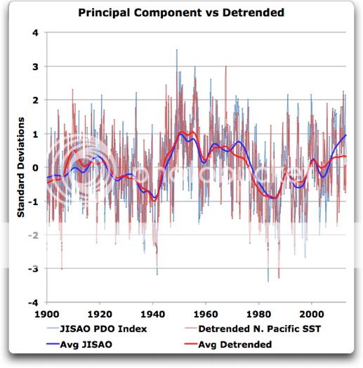
Then, instead of taking the principal components, I simply detrended the result. Here is the comparison, between a simple detrend and the principal component method.
Now, you may recall my statement was as follows:
The actual data shown above is a complete confirmation of my claim. The JISAO PDO Index, calculated as the principal component of the SST data, is indeed quite similar to the simple detrend of the same data (correlation = 0.76). And if I had the actual dataset they used, instead of using the HadISST, the similarity would be even greater.
Both you and Paul have told me, at times in rather unpleasant fashion, that I was misunderstanding the situation … I’ll gladly accept an apology from either or both of you. It turns out that I understood what I was saying very well, and it was you and Paul who were wrong. I may be self-educated, which has its own problems, but as a result I’ve noticed a few things that the professionally trained folks such as you two might have missed in your education …
w.
dp, once tropical storms get heat in to middle upper troposphere a significant amount will be lost to space. Rest goes polewards by Hadley convection.
Warmer SST will radiate all along the path, leaving some residual effect at high latitudes.
there it will melt ice , increase open sea area and increase direct radiative loss to space and increase evaporation.
W. Pacific wind speed reflects SST at the point Willis describes as the splitting of tropical currents to go north and south. Note the 5.42 year peak:
http://climategrog.wordpress.com/?attachment_id=281
The same period of 5.42 years can be found in the rate of change in arctic ice area:
http://climategrog.wordpress.com/2013/03/11/open-mind-or-cowardly-bigot/ddt_arctic_ice/
So, no it’s equal to… there are many ways the heat dissipates, but changes in W. Pacific can be seen reflected in observable data at the pole.
“Both you and Paul have told me, at times in rather unpleasant fashion, that I was misunderstanding the situation … I’ll gladly accept an apology from either or both of you.”
I think I told rather politely that you were misunderstanding the situation. You still are.
The step that you have missed despite have quoted it and spelt it out is the” I subtracted the monthly mean global average SST anomalies, just as the JISAO folks did” bit.
That is where the “something like detrending” comes from not the EOF.
I’ll gladly accept an apology (and thanks for all the time I’ve spent patiently explaining this so that you don’t need to google to find out what EOF is for yourself) 😉
Like I’ve said before , don’t take it the wrong way when I correct some aspect when you get something a bit wrong. You come up with some good stuff and it would be more robust to criticism if you got the maths/physics right. You do most of the time. If I correct you on something it’s to reinforce it, not try to get one over on you because your self-educated.
Most of the important things I know are self taught and I’m pretty much like yourself. When I need to do something , I find out and I do it. I’ve no disrespect for that.
Greg Goodman says:
June 9, 2013 at 3:32 pm
I fear I don’t understand that. I followed their procedures, right up to the point where they calculated the PC and I used the detrend. The results were very similar. You say I missed a step … what step did I miss? Here are the two procedures
THEIR PROCEDURE
Take the N. Pacific SSTs
Subtract the global SSTs
Take the principal components
MY PROCEDURE
Take the N. Pacific SSTs
Subtract the global SSTs
Detrend
The results are very similar … what step am I skipping?
What am I not seeing here? How did I get to something so similar their PC results by using a simple detrend, if (as you and Paul claim) they should not be similar?
Your explanation explains nothing.
w.
@Willis 1:51 pm –
About SABRE: http://www.nasa.gov/topics/earth/features/AGU-SABER.html
Pretty cool stuff. And a perhaps significant step forward, adding an entirely new element to the climate change debate. With a non-constant atmospheric radiation budget, the legs might be knocked out from under current assumptions.
Steve Garcia
Oops! A H/T Eric Eikenberry who pointed all that out to Willis…
Steve Garcia
I did not say you were skipping a step in the processing. I meant you were missing the significance of something you had described doing: ‘The step that you have missed despite have quoted it and spelt it out is the” I subtracted the monthly mean global average SST anomalies” bit’.
You are missing the fact that a step (common to both) is subtracting the global mean, That has a “similar” trend to N.P. data and is effectively detrending it. You’ll probalby find your additional detrending did not make much difference after that.
The EOF is just like a fancy way of getting an average kind of series that is “typical” of the data.
Thanks for your answer Bob and the links. Willis doesn’t seem to be interested in the NOAA 1000 year reconstruction.
Perhaps I’ll try again another day.
Here is a link to the foundational paper on self-organised criticality by Bak, Tang and Weisefeld (“BTW 1987”):
http://webber.physik.uni-freiburg.de/~jeti/studenten_seminar/stud_sem05/bak.pdf
This points to the establishment of attractors in open dissipative systems. The PDO is an example of such an attractor.
In this paper, we argue and demonstrate numerically that dynamical systens with extended spatial degrees of freedom naturally evolve into self-organising critical structures of states which are barely stable. We suggest that this self-organising criticality is the common underlying mechanism behind the phenomena described above. The combination of dynamical minimal stability and spatial scaling leads to a power law for temporal fluctuations. The noise propagates through the scaling structures by means of a “domino” effect upsetting the minimally stable states. Long wavelength perturbations cause a cascade of energy dissipation on all scales, which is the main characteristic of turbulence.
A “power law for temporal fluctuations” in climate demands oscillation on the timescale of the PDO as it does on all timescales.
Eric Eikenberry says:
June 9, 2013 at 11:30 am
“If you’re looking for a controlling “trigger”, the very fact that the atmosphere can and does expand and contract should be considered a major factor. This must have an effect on the jet stream patterns, and by default, the PDO through cloud cover placement due to the jet stream.”
Joule heating of the upper atmosphere apparently causes strong circulation in the polar regions which appears to have a strong influence on the Arctic Oscillation and hence the jet stream, and as you say, the PDO: http://www.arctic.noaa.gov/detect/detection-images/climate-ao_nov-mar_2011-600.png
A complex oscillation with alternating periods dominated statistically (but in a messy sort of way) by high fluctuations (el Nino) and low fluctuations (La Nina) – it looks very like a Lorenz attractor.
As proposed here a couple of years ago.
Ulric Lyons says: “Joule heating of the upper atmosphere apparently causes strong circulation in the polar regions which appears to have a strong influence on the Arctic Oscillation…”
AO leads d/dt(CO2) at Mauna Loa !
http://climategrog.wordpress.com/?attachment_id=227
and d/dt(CO2) correlates with global mean SST :
http://climategrog.wordpress.com/?attachment_id=223
any more specifics on that Joule heating ‘influencing’ AO ? Numbers?