Guest Post by Willis Eschenbach
I haven’t commented much on my most recents posts, because of the usual reasons: a day job, and the unending lure of doing more research, my true passion. To be precise, recently I’ve been frying my synapses trying to twist my head around the implications of the finding that the global temperature forecasts of the climate models are mechanically and accurately predictable by a one-line equation. It’s a salutary warning: kids, don’t try climate science at home.
 Figure 1. What happens when I twist my head too hard around climate models.
Three years ago, inspired by Lucia Liljegren’s ultra-simple climate model that she called “Lumpy”, and with the indispensable assistance of the math-fu of commenters Paul_K and Joe Born, I made what to me was a very surprising discovery. The GISSE climate model could be accurately replicated by a one-line equation. In other words, the global temperature output of the GISSE model is described almost exactly by a lagged linear transformation of the input to the models (the “forcings” in climatespeak, from the sun, volcanoes, CO2 and the like). The correlation between the actual GISSE model results and my emulation of those results is 0.98 … doesn’t get much better than that. Well, actually, you can do better than that, I found you can get 99+% correlation by noting that they’ve somehow decreased the effects of forcing due to volcanoes. But either way, it was to me a very surprising result. I never guessed that the output of the incredibly complex climate models would follow their inputs that slavishly.
Since then, Isaac Held has replicated the result using a third model, the CM2.1 climate model. I have gotten the CM2.1 forcings and data, and replicated his results. The same analysis has also been done on the GDFL model, with the same outcome. And I did the same analysis on the Forster data, which is an average of 19 model forcings and temperature outputs. That makes four individual models plus the average of 19 climate models, and all of the the results have been the same, so the surprising conclusion is inescapable—the climate model global average surface temperature results, individually or en masse, can be replicated with over 99% fidelity by a simple, one-line equation.
However, the result of my most recent “black box” type analysis of the climate models was even more surprising to me, and more far-reaching.
Here’s what happened. I built a spreadsheet, in order to make it simple to pull up various forcing and temperature datasets and calculate their properties. It uses “Solver” to iteratively select the values of tau (the time constant) and lambda (the sensitivity constant) to best fit the predicted outcome. After looking at a number of results, with widely varying sensitivities, I wondered what it was about the two datasets (model forcings, and model predicted temperatures) that determined the resulting sensitivity. I wondered if there were some simple relationship between the climate sensitivity, and the basic statistical properties of the two datasets (trends, standard deviations, ranges, and the like). I looked at the five forcing datasets that I have (GISSE, CCSM3, CM2.1, Forster, and Otto) along with the associated temperature results. To my total surprise, the correlation between the trend ratio (temperature dataset trend divided by forcing dataset trend) and the climate sensitivity (lambda) was 1.00. My jaw dropped. Perfect correlation? Say what? So I graphed the scatterplot.
 Figure 2. Scatterplot showing the relationship of lambda and the ratio of the output trend over the input trend. Forster is the Forster 19-model average. Otto is the Forster input data as modified by Otto, including the addition of a 0.3 W/m2 trend over the length of the dataset. Because this analysis only uses radiative forcings and not ocean forcings, lambda is the transient climate response (TCR). If the data included ocean forcings, lambda would be the equilibrium climate sensitivity (ECS). Lambda is in degrees per W/m2 of forcing. To convert to degrees per doubling of CO2, multiply lambda by 3.7.
Dang, you don’t see that kind of correlation very often, R^2 = 1.00 to two decimal places … works for me.
Let me repeat the caveat that this is not talking about real world temperatures. This is another “black box” comparison of the model inputs (presumably sort-of-real-world “forcings” from the sun and volcanoes and aerosols and black carbon and the rest) and the model results. I’m trying to understand what the models do, not how they do it.
Now, I don’t have the ocean forcing data that was used by the models. But I do have Levitus ocean heat content data since 1950, poor as it might be. So I added that to each of the forcing datasets, to make new datasets that do include ocean data. As you might imagine, when some of the recent forcing goes into heating the ocean, the trend of the forcing dataset drops … and as we would expect, the trend ratio (and thus the climate sensitivity) increases. This effect is most pronounced where the forcing dataset has a smaller trend (CM2.1) and less visible at the other end of the scale (CCSM3). Figure 3 shows the same five datasets as in Figure 2, plus the same five datasets with the ocean forcings added. Note that when the forcing dataset contains the heat into/out of the ocean, lambda is the equilibrium climate sensitivity (ECS), and when the dataset is just radiative forcing alone, lambda is transient climate response. So the blue dots in Figure 3 are ECS, and the red dots are TCR. The average change (ECS/TCR) is 1.25, which fits with the estimate given in the Otto paper of ~ 1.3.
 Figure 3. Red dots show the models as in Figure 2. Blue dots show the same models, with the addition of the Levitus heat content data to each forcing dataset. Resulting sensitivities are higher for the equilibrium condition than for the transient condition, as would be expected. Blue dots show equilibrium climate sensitivity (ECS), while red dots (as in Fig. 2) show the corresponding transient climate response (TCR).
Finally, I ran the five different forcing datasets, with and without ocean forcing, against three actual temperature datasets—HadCRUT4, BEST, and GISS LOTI. I took the data from all of those, and here are the results from the analysis of those 29 individual runs:
 Figure 4. Large red and blue dots are as in Figure 3. The light blue dots are the result of running the forcings and subsets of the forcings, with and without ocean forcing, and with and without volcano forcing, against actual datasets. Error shown is one sigma.
So … my new finding is that the climate sensitivity of the models, both individual models and on average, is equal to the ratio of the trends of the forcing and the resulting temperatures. This is true whether or not the changes in ocean heat content are included in the calculation. It is true for both forcings vs model temperature results, as well as forcings run against actual temperature datasets. It is also true for subsets of the forcing, such as volcanoes alone, or for just GHG gases.
And not only did I find this relationship experimentally, by looking at the results of using the one-line equation on models and model results. I then found that can derive this relationship mathematically from the one-line equation (see Appendix D for details).
This is a clear confirmation of an observation first made by Kiehl in 2007, when he suggested an inverse relationship between forcing and sensitivity.
The question is: if climate models differ by a factor of 2 to 3 in their climate sensitivity, how can they all simulate the global temperature record with a reasonable degree of accuracy. Kerr [2007] and S. E. Schwartz et al. (Quantifying climate change–too rosy a picture?, available [here]) recently pointed out the importance of understanding the answer to this question. Indeed, Kerr [2007] referred to the present work, and the current paper provides the ‘‘widely circulated analysis’’ referred to by Kerr [2007]. This report investigates the most probable explanation for such an agreement. It uses published results from a wide variety of model simulations to understand this apparent paradox between model climate responses for the 20th century, but diverse climate model sensitivity.
However, Kiehl ascribed the variation in sensitivity to a difference in total forcing, rather than to the trend ratio, and as a result his graph of the results is much more scattered.
 Figure 5. Kiehl results, comparing climate sensitivity (ECS) and total forcing. Note that unlike Kiehl, my results cover both equilibrium climate sensitivity (ECS) and transient climate response (TCR).
Anyhow, there’s a bunch more I could write about this finding, but I gotta just get this off my head and get back to my day job. A final comment.
Since I began this investigation, the commenter Paul_K has since written two outstanding posts on the subject over at Lucia’s marvelous blog, The Blackboard (Part 1, Part 2). In those posts, he proves mathematically that given what we know about the equation that replicates the climate models, that we cannot … well, I’ll let him tell it in his own words:
The Question: Can you or can you not estimate Equilibrium Climate Sensitivity (ECS) from 120 years of temperature and OHC data (even) if the forcings are known?
The Answer is: No. You cannot. Not unless other information is used to constrain the estimate.
An important corollary to this is:- The fact that a GCM can match temperature and heat data tells us nothing about the validity of that GCM’s estimate of Equilibrium Climate Sensitivity.
Note that this is not an opinion of Paul_K’s. It is a mathematical result of the fact that even if we use a more complex “two-box” model, we can’t constrain the sensitivity estimates. This is a stunning and largely unappreciated conclusion. The essential problem is that for any given climate model, we have more unknowns than we have fundamental equations to constrain them.
CONCLUSIONS
Well, it was obvious from my earlier work that the models were useless for either hindcasting or forecasting the climate. They function indistinguishably from a simple one-line equation.
On top of that, Paul_K has shown that they can’t tell us anything about the sensitivity, because the equation itself is poorly constrained.
Finally, in this work I’ve shown that the climate sensitivity “lambda” that the models do exhibit, whether it represents equilibrium climate sensitivity (ECS) or transient climate response (TCR), is nothing but the ratio of the trends of the input and the output. The choice of forcings, models and datasets is quite immaterial. All the models give the same result for lambda, and that result is the ratio of the trends of the forcing and the response. This most recent finding completely explains the inability of the modelers to narrow the range of possible climate sensitivities despite thirty years of modeling.
You can draw your own conclusions from that, I’m sure …
My regards to all,
w.
Appendix A : The One-Line Equation
The equation that Paul_K, Isaac Held, and I have used to replicate the climate models is as follows:
![]()
Let me break this into four chunks, separated by the equals sign and the plus signs, and translate each chunk from math into English. Equation 1 means:
This year’s temperature (T1) is equal to
Last years temperature (T0) plus
Climate sensitivity (λ) times this year’s forcing change (∆F1) times (one minus the lag factor) (1-a) plus
Last year’s temperature change (∆T0) times the same lag factor (a)
Or to put it another way, it looks like this:
T1 = <— This year’s temperature [ T1 ] equals
T0 + <— Last year’s temperature [ T0 ] plus
λ ∆F1 (1-a) + <— How much radiative forcing is applied this year [ ∆F1 (1-a) ], times climate sensitivity lambda ( λ ), plus
∆T0 a <— The remainder of the forcing, lagged out over time as specified by the lag factor “a”
The lag factor “a” is a function of the time constant “tau” ( τ ), and is given by
![]()
This factor “a” is just a constant number for a given calculation. For example, when the time constant “tau” is four years, the constant “a” is 0.78. Since 1 – a = 0.22, when tau is four years, about 22% of the incoming forcing is added immediately to last years temperature, and rest of the input pulse is expressed over time.
Appendix B: Physical Meaning
So what does all of that mean in the real world? The equation merely reflects that when you apply heat to something big, it takes a while for it to come up to temperature. For example, suppose we have a big brick in a domestic oven at say 200°C. Suppose further that we turn the oven heat up suddenly to 400° C for an hour, and then turn the oven back down to 200°C. What happens to the temperature of the big block of steel?
If we plot temperature against time, we see that initially the block of steel starts to heat fairly rapidly. However as time goes on it heats less and less per unit of time until eventually it reaches 400°C. Figure B2 shows this change of temperature with time, as simulated in my spreadsheet for a climate forcing of plus/minus one watt/square metre. Now, how big is the lag? Well, in part that depends on how big the brick is. The larger the brick, the longer the time lag will be. In the real planet, of course, the ocean plays the part of the brick, soaking up
The basic idea of the one-line equation is the same tired claim of the modelers. This is the claim that the changing temperature of the surface of the planet is linearly dependent on the size of the change in the forcing. I happen to think that this is only generally the rule, and that the temperature is actually set by the exceptions to the rule. The exceptions to this rule are the emergent phenomena of the climate—thunderstorms, El Niño/La Niña effects and the like. But I digress, let’s follow their claim for the sake of argument and see what their models have to say. It turns out that the results of the climate models can be described to 99% accuracy by the setting of two parameters—”tau”, or the time constant, and “lambda”, or the climate sensitivity. Lambda can represent either transient sensitivity, called TCR for “transient climate response”, or equilibrium sensitivity, called ECS for “equilibrium climate sensitivity”.
 Figure B2. One-line equation applied to a square-wave pulse of forcing. In this example, the sensitivity “lambda” is set to unity (output amplitude equals the input amplitude), and the time constant “tau” is set at five years.
Note that the lagging does not change the amount of energy in the forcing pulse. It merely lags it, so that it doesn’t appear until a later date.
So that is all the one-line equation is doing. It simply applies the given forcing, using the climate sensitivity to determine the amount of the temperature change, and using the time constant “tau” to determine the lag of the temperature change. That’s it. That’s all.
The difference between ECS (climate sensitivity) and TCR (transient response) is whether slow heating and cooling of the ocean is taken into account in the calculations. If the slow heating and cooling of the ocean is taken into account, then lambda is equilibrium climate sensitivity. If the ocean doesn’t enter into the calculations, if the forcing is only the radiative forcing, then lambda is transient climate response.
Appendix C. The Spreadsheet
In order to be able to easily compare the various forcings and responses, I made myself up an Excel spreadsheet. It has a couple drop-down lists that let me select from various forcing datasets and various response datasets. Then I use the built-in Excel function “Solver” to iteratively calculate the best combination of the two parameters, sensitivity and time constant, so that the result matches the response. This makes it quite simple to experiment with various combinations of forcing and responses. You can see the difference, for example, between the GISS E model with and without volcanoes. It also has a button which automatically stores the current set of results in a dataset which is slowly expanding as I do more experiments.
In a previous post called Retroactive Volcanoes, (link) I had discussed the fact that Otto et al. had smoothed the Forster forcings dataset using a centered three point average. In addition they had added a trend fromthe beginning tothe end of the dataset of 0.3 W per square meter. In that post I had I had said that the effect of that was unknown, although it might be large. My new spreadsheet allows me to actually determine what the effect of that actually is.
It turns out that the effect of those two small changes is to take the indicated climate sensitivity from 2.8 degrees/doubling to 2.3° per doubling.
One of the strangest findings to come out of this spreadsheet was that when the climate models are compared each to their own results, the climate sensitivity is a simple linear function of the ratio of the trends of the forcing and the response. This was true of both the individual models, and the average of the 19 models studied by Forster. The relationship is extremely simple. The climate sensitivity lambda is 1.07 times the ratio of the trends for the models alone, and equal to the trends when compared to all the results. This is true for all of the models without adding in the ocean heat content data, and also all of the models including the ocean heat content data.
In any case I’m going to have to convert all this to the computer language R. Thanks to Stephen McIntyre, I learned the computer language R and have never regretted it. However, I still do much of my initial exploratory forays in Excel. I can make Excel do just about anything, so for quick and dirty analyses like the results above I use Excel.
So as an invitation to people to continue and expand this analysis, my spreadsheet is available here. Note that it contains a macro to record the data from a given analysis. At present it contains the following data sets:
IMPULSES
Pinatubo in 1900
Step Change
Pulse
FORCINGS
Forster No Volcano
Forster N/V-Ocean
Otto Forcing
Otto-Ocean ∆
Levitus watts Ocean Heat Content ∆
GISS Forcing
GISS-Ocean ∆
Forster Forcing
Forster-Ocean ∆
DVIS
CM2.1 Forcing
CM2.1-Ocean ∆
GISS No Volcano
GISS GHGs
GISS Ozone
GISS Strat_H20
GISS Solar
GISS Landuse
GISS Snow Albedo
GISS Volcano
GISS Black Carb
GISS Refl Aer
GISS Aer Indir Eff
RESPONSES
CCSM3 Model Temp
CM2.1 Model Temp
GISSE ModelE Temp
BEST Temp
Forster Model Temps
Forster Model Temps No Volc
Flat
GISS Temp
HadCRUT4
You can insert your own data as well or makeup combinations of any of the forcings. I’ve included a variety of forcings and responses. This one-line equation model has forcing datasets, subsets of those such as volcanoes only or aerosols only, and the simple impulses such as a square step.
Now, while this spreadsheet is by no means user-friendly, I’ve tried to make it at least not user-aggressive.
Appendix D: The Mathematical Derivation of the Relationship between Climate Sensitivity and the Trend Ratio.
I have stated that the relationship where climate sensitivity is equal to the ratio between trends of the forcing and response datasets.
We start with the one-line equation:
![]()
Let us consider the situation of a linear trend in the forcing, where the forcing is ramped up by a certain amount every year. Here are lagged results from that kind of forcing.

Figure B1. A steady increase in forcing over time (red line), along with the situation with the time constant (tau) equal to zero, and also a time constant of 20 years. The residual is offset -0.6 degrees for clarity.
Note that the only difference that tau (the lag time constant) makes is how long it takes to come to equilibrium. After that the results stabilize, with the same change each year in both the forcing and the temperature (∆F and ∆T). So let’s consider that equilibrium situation.
Subtracting T0 from both sides gives
![]()
Now, T1 minus T0 is simply ∆T1. But since at equilibrium all the annual temperature changes are the same, ∆T1 = ∆T0 = ∆T, and the same is true for the forcing. So equation 2 simplifies to
![]()
Dividing by ∆F gives us

Collecting terms, we get

And dividing through by (1-a) yields

Now, out in the equilibrium area on the right side of Figure B1, ∆T/∆F is the actual trend ratio. So we have shown that at equilibrium

But if we include the entire dataset, you’ll see from Figure B1 that the measured trend will be slightly less than the trend at equilibrium.
And as a result, we would expect to find that lambda is slightly larger than the actual trend ratio. And indeed, this is what we found for the models when compared to their own results, lambda = 1.07 times the trend ratio.
When the forcings are run against real datasets, however, it appears that the greater variability of the actual temperature datasets averages out the small effect of tau on the results, and on average we end up with the situation shown in Figure 4 above, where lambda is experimentally determined to be equal to the trend ratio.
Appendix E: The Underlying Math
The best explanation of the derivation of the math used in the spreadsheet is an appendix to Paul_K’s post here. Paul has contributed hugely to my analysis by correcting my mistakes as I revealed them, and has my great thanks.
Climate Modeling – Abstracting the Input Signal by Paul_K
I will start with the (linear) feedback equation applied to a single capacity system—essentially the mixed layer plus fast-connected capacity:
C dT/dt = F(t) – λ *T Equ. A1
Where:-
C is the heat capacity of the mixed layer plus fast-connected capacity (Watt-years.m-2.degK-1)
T is the change in temperature from time zero (degrees K)
T(k) is the change in temperature from time zero to the end of the kth year
t is time (years)
F(t) is the cumulative radiative and non-radiative flux “forcing” applied to the single capacity system (Watts.m-2)
λ is the first order feedback parameter (Watts.m-2.deg K-1)
We can solve Equ A1 using superposition. I am going to use timesteps of one year.
Let the forcing increment applicable to the jth year be defined as fj. We can therefore write
F(t=k ) = Fk = Σ fj for j = 1 to k Equ. A2
The temperature contribution from the forcing increment fj at the end of the kth
year is given by
ΔTj(t=k) = fj(1 – exp(-(k+1-j)/τ))/λ Equ.A3
where τ is set equal to C/λ .
By superposition, the total temperature change at time t=k is given by the summation of all such forcing increments. Thus
T(t=k) = Σ fj * (1 – exp(-(k+1-j)/τ))/ λ for j = 1 to k Equ.A4
Similarly, the total temperature change at time t= k-1 is given by
T(t=k-1) = Σ fj (1 – exp(-(k-j)/τ))/ λ for j = 1 to k-1 Equ.A5
Subtracting Equ. A4 from Equ. A5 we obtain:
T(k) – T(k-1) = fk*[1-exp(-1/τ)]/λ + ( [1 – exp(-1/τ)]/λ ) (Σfj*exp(-(k-j)/τ) for j = 1 to k-1) …Equ.A6
We note from Equ.A5 that
(Σfj*exp(-(k-j)/τ)/λ for j = 1 to k-1) = ( Σ(fj/λ ) for j = 1 to k-1) – T(k-1)
Making this substitution, Equ.A6 then becomes:
T(k) – T(k-1) = fk*[1-exp(-1/τ)]/λ + [1 – exp(-1/τ)]*[( Σ(fj/λ ) for j = 1 to k-1) – T(k-1)] …Equ.A7
If we now set α = 1-exp(-1/τ) and make use of Equ.A2, we can rewrite Equ A7 in the following simple form:
T(k) – T(k-1) = Fkα /λ – α * T(k-1) Equ.A8
Equ.A8 can be used for prediction of temperature from a known cumulative forcing series, or can be readily used to determine the cumulative forcing series from a known temperature dataset. From the cumulative forcing series, it is a trivial step to abstract the annual incremental forcing data by difference.
For the values of α and λ, I am going to use values which are conditioned to the same response sensitivity of temperature to flux changes as the GISS-ER Global Circulation Model (GCM).
These values are:-
α = 0.279563
λ = 2.94775
Shown below is a plot confirming that Equ. A8 with these values of alpha and lamda can reproduce the GISS-ER model results with good accuracy. The correlation is >0.99.

This same governing equation has been applied to at least two other GCMs ( CCSM3 and GFDL ) and, with similar parameter values, works equally well to emulate those model results. While changing the parameter values modifies slightly the values of the fluxes calculated from temperature , it does not significantly change the structural form of the input signal, and nor can it change the primary conclusion of this article, which is that the AGW signal cannot be reliably extracted from the temperature series.
Equally, substituting a more generalised non-linear form for Equ A1 does not change the results at all, provided that the parameters chosen for the non-linear form are selected to show the same sensitivity over the actual observed temperature range. (See here for proof.)
Yes I agree climate models based on the political decided UNFCCC are unscientific and are with 99 % certainty WRONG
Hi Willis,
This is fairly common in engineering (that a complex system can be modeled by a simple equation over limited conditions/time-frame). As useful as that can be, it does not demonstrate understanding of the complex system- it merely means you can predict behavior over some limited range. OK, so what? Well, often that’s good enough. I’ll say that again, often that’s good enough.
The problem is when a real event occurs that invalidates the simple equation (black box) and the black box no longer produces useful output. So there’s a difference between something that’s useful, and really understanding what’s under the hood.
In the long run, you are better off understanding the complex system, but folks should understand that’s not required for something to be useful.
it is their way to keep energy conservation under control?
Matthew R Marler says:
June 3, 2013 at 12:23 pm
Apologies for the lack of clarity, Matt, I should have said “steady state” rather than “equilibrium”, as the forcing and temperature are both continually rising (see figure B1).
w.
Willis, I think you have found an underlying fact about the current status of climate science. Since 1980’s there has really been only cosmetic changes in AGR predictions despite an order of magnitude increase in resolution and complexity of GCM models. Most of the “progress” (IMHO) seems to have been in fine tuning various “natural/anthropogenic” variations in aerosols to better fit past temperature response. Uncertainties still remain about natural feedbacks – especially clouds. Looking at your equation.
 where
where  is the transient temperature response and
  is the equilibrium temperature response.


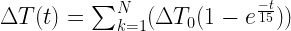
 , where C and C0 are the values before and after the yearly pulse. All values are calculated from seasonally averaged Mauna Loa data smoothed back to an initial concentration of 280ppm in 1750.
 was calculated based on an assumed ECS of 2.0C. The results can then be compared to the observed HADCRUT4 temperature anomalies – see here.
Tau is the relaxation time for the climate system to react to any sudden change in forcing. This could be a volcano, a meteor, aerosols or CO2. Climate models including ocean/atmosphere interactions (for example GISS) seem to point to a value for Tau of ~ 10-15 years. Your equation works by simply taking direct CO2 forcing (MODTRAN) each year to be DF = 5.3ln(C/C0), where C-C0 = the increase measured using the Mauna Loa data extrapolated back to 1750. So simply taking lambda as the climate sensitivity (hoping latex works!)
and then taking Stefan Boltzman to derive the IR energy balance
or in terms of feedbacks
and for equilibrium climate sensitivity for a doubling of CO2
To calculate the CO2 forcing take a yearly increment of
Each pulse is tracked through time and integrated into the overall transient temperature change using:
If we assume an underlying 60 year natural oscillation (AMO?) superimposed onto a CO2 AGW signal then at worst ECS works out to be ~2C.
more details – here
One line equations may work to emulate the crude GISS models but there is talk around town that the NCAR/UCAR CESM takes computational and algorithmic advantage of the vibrations of the massive crystal dome under the City of Boulder. There is no way to simplify and match that.
which is that the climate sensitivity given by the climate models is simply the trend ratio …
======
woops…..so even if they are putting in all of the other crap……all that stuuf is doing is cancelling itself out
If 2 computer systems are functionally equivalent, that is they produce the same outputs from the same inputs, then they are logically equivalent, that is the operations of one can be transformed into the operations of the other.
Which means 99.99% of the code in the climate models doesn’t actually do anything significant to the outputs. And buried within them is the logical equivalent of Willis’ equation.
The climate modellers must surely know this.
Roy Spencer says:
June 3, 2013 at 12:33 pm
Coming from a simulation background I’ve been saying for years that all they did was pick a CS they liked, and then adjusted the other knobs until they liked the results.
But what’s really telling is that their 3D results aren’t very good, it’s only when they average them all together that they have something they can print while not hiding their faces.
and
Basically they can’t simulate any random specific area correctly, but it’s close if they average all of their errors together.
So essentially, we have paid a trillion dollars for this equation and published (apparently) 100,000+ papers on it, and Willis has reduced all the bumph down to an equation with an R^2 fit of 1.00. Mosher says this is nothing new here, but in the previous post when Willis used this equation as the blackbox equation, he protested that this isn’t the equation used by IPCC nobility – a disengenuous critique, with what he apparently knew already. Roy Spencer made the same criticism but I would argue to these two gentlemen that all the rest of us got a hell of a good education out of his effort because those in the know weren’t prepared to present this revelation to the great unwashed. The consensus synod has less to sneer and much to fear from the work of this remarkable man.
MJB says:
June 3, 2013 at 12:31 pm
“of funding. I don’t have the reference in front of me, but I recall at least one GCM being criticized for including an interactive “solver” type application integrated into the parameter setting process to handle just such gaming.”
WHAT? It is frowned upon when they train the parameterization automatically? It is expected that they do it manually? What for? To uphold a pretense of scientific activity? The cult is getting ridiculouser by the day.
In electronics, Thevenin’s* theorem states that any linear black box circuit, no matter how complicated, can be replaced with a voltage source and an impedance. Since a linear circuit, no matter how complicated, is modeled by a set of linear equations, we can extrapolate that any set of linear equations can be replaced by one linear equation if all we want is the overall system response.
Your results make it a pretty good bet that the climate models are predominantly linear. Given that we’re talking about thermodynamics, … yep, I think that might be a problem.
=============================================
*http://en.wikipedia.org/wiki/Th%C3%A9venin%27s_theorem Thevenin is a great shortcut for circuit analysis, nothing more.
Steven Mosher says:
June 3, 2013 at 12:04 pm
“err
I pointed this out to you back in 2008
http://climateaudit.org/2008/05/09/giss-model-e-data/#comment-148141
http://rankexploits.com/musings/2008/lumpy-vs-model-e/
nothing surprising about this. You can fit the super complicated Line by Line radiative transfer models with a simple function delta forcing = 5.35ln(C02a/C02b)”
_____________________
You really should ripen those sour grapes before you try to sell ’em… they are (again) making it appear that you are attempting obfuscation.
~~~~~~~~~~~~~~~~~~~~~
MiCro says:
June 3, 2013 at 1:35 pm
“Coming from a simulation background I’ve been saying for years that all they did was pick a CS they liked, and then adjusted the other knobs until they liked the results.”
_________________________
Yes indeed. That’s the way it’s looked for quite some time. (won’t mention harryreadme)
~~~~~~~~~~~~~~~~~~~~~~~~~
Willis Eschenbach says:
June 3, 2013 at 1:14 pm
Matthew R Marler says:
June 3, 2013 at 12:23 pm
“But since at equilibrium all the annual temperature changes are the same, ∆T1 = ∆T0 = ∆T, and the same is true for the forcing.
At equilibrium, all of the temperature changes and forcing changes are 0. The first is the definition of equilibrium,, and the second is one of the necessary conditions for an equilibrium to be possible.”
“Apologies for the lack of clarity, Matt, I should have said “steady state” rather than “equilibrium”, as the forcing and temperature are both continually rising (see figure B1).”
w.
__________________
Fine work, nevertheless. Many thanks.
~~~~~~~~~~~~~~~~~~~~
The fact that a GCM can match temperature and heat data tells us nothing about the validity of that GCM’s estimate of Equilibrium Climate Sensitivity.
+++++++++++++++++
Only the climate models with the correct Equilibrium Climate Sensitivity would be able hind-cast past temperatures. However, multiple models with different ECS can all hind-cast past temperatures. Which either means that ECS doesn’t determine temperature, or the models are faulty.
Matthew R Marler says:
June 3, 2013 at 12:23 pm
As you wrote, you have modeled the models, but you have not modeled the climate.
========
since it is quite clear that the models haven’t modeled climate, anything that models the models is also not going to model climate.
The models are pretty simple really. Each cell in the atm has a set of inputs and outputs on each side, plus top and bottom. There’s a set of rules that does the math based on each in, and propagates the results to each output. There are cells who’s sides are dirt, and by now ones who’s sides are water. There are 14-15 cells for each area from the a little below the surface up to space. And a grid of cells to cover the earth, the more cells the more accurate the results are, but the longer the simulations take to run. Climatologists have been insisting that the reason they’re results are off is they can’t make the grids small enough. So bigger computers are required.
When it’s initialize, without stepping “time”, inputs are propagated to output until the outputs become stable. This accounts for the output of one cell changing the input of another. They do this until each cell initialized to the state it’s defined to be, then they provide a forcing, and let the clock step forward one clock tick, then each cell runs it’s calculations until the output stabilizes. Then they step the clock, and repeat.
This is the same process used by linear simulators like SPICE, in fact you could replicate the equations of each cell with spice, it would just be really slow, and more difficult to twist knobs on.
But it’s just a bunch of equations to solve.
This link is to a very good document on the basics of GCM’s.
commieBob says:
June 3, 2013 at 1:53 pm
“Thevenin’s theorum…”
_____________________
Yep. I’ve never been able to look at the any statement about climate models without visions of Thevenin- Norton equivalents and Kirchoff equations zapping through what’s left of my brain.
Philip Bradley says:
June 3, 2013 at 1:33 pm
I
I doubt it. The climate models, like Topsy, have “jes’ growed”. In addition, it’s a recurring problem with iterative models, which is that even if you get the “right” answer, you don’t know how you got there … but my “black box” analysis shows how. So I don’t think the modelers knew that.
w.
Nice work, Willis and collaborators. As with all clear math, beautiful and compelling.
Another answer to Dr. Spencer is that his comment applies to figure three, but not to an important part of figure four and smacks of sour grapes, especially since his own recent simple model did not work out so well.
A comment is surprising that so many different GCM models (and an ensemble!) gave ‘exactly’ the same trend ratio answer to the relationship between forcing input and temperature output, even though from figures two and three obviously not the same lambda, showing the models themselves do differ in important sensitivity respects (itself primarily driven by positive water vapor feedback and clouds, since the ‘feedback neutral’ sensitivity from Stefan-Boltsmann is always between 1( theoretical black body) and model grid specific, real earth ‘grey body’ 1.2).
A possible reason is that each model is ‘tuned’ (parameterized with things like aerosols and within grid cell cloud and convection microprocesses) to hind cast past temperature as accurately as possible. Even though those tunings differ by model, they all produce the same temperature result, so by intent the same trend ratio as evidenced in Figures 2 and 3. Another way to show that they are therefore unlikely to accurately predict the future temperature or true sensitivity, as you have already observed.
It will be most interesting to learn what you and your collaborators do next with these most interesting results. One suggestion might be to use the one line equation and it’s corollaries to ‘filter out’ the known forcings (like CO2) temperature consequences to estimate the ‘natural’ variability of temperature over the periods where data of different levels of certainty exists. Satellite era greatest, 1880 or so least. Said differently your new tools might go a long way on the attribution problem. Can a 60 year natural cycle be extracted? Can the pause be explained as a function of whatever happened from 1945-1965? Lots of potentially interesting stuff, without spending more billions to spin up the supercomputers for months at a pass.
Willis,
“So … my new finding is that the climate sensitivity of the models, both individual models and on average, is equal to the ratio of the trends of the forcing and the resulting temperatures.”
I think calculus gives a reason for this. Idealized,
trend_T≅dT/dt, trend_F≅dF/dt
and, with many caveats as discussed in your previous thread,
λ≅dT/dF=(dT/dt)/(dF/dt)=trend_T/trend_F
Willis – I am surprised that you are surprised by what you found. It is an inevitable result of their process.. See IPCC report AR4 Ch.9 Executive Summary : “Estimates of the climate sensitivity are now better constrained by observations.“. “constrained by observation” means that they constrained their models in order to get climate sensitivity to match observed temperature. Forcings are the primary inputs to the models, so across the models you must necessarily get the relationship that you noticed.
Rud Istvan says:
June 3, 2013 at 2:09 pm
Thanks for your kind words, Rud. I wish I had collaborators, it’s just me and my computer.
Regarding what’s next, I want to apply the equations on a gridcell-by-gridcell basis using the CERES data. As you point out, the interesting thing about the one-line equation is that we can use it to see both when and where the climate is NOT responding as expected to the forcing.
w.
Rud Istvan says:
June 3, 2013 at 2:09 pm
This is because they’re all almost identical, at most they adjust the equations in the cells, mostly they just set the knobs differently.
Mod, I think my last post got eaten, can you check for it? this post will make more sense after reading the last one.
[Reply: Prior comment found in Spam folder. Rescued & posted. — mod.]
Colorado Wellington says:
June 3, 2013 at 1:21 pm
One line equations may work to emulate the crude GISS models but there is talk around town that the NCAR/UCAR CESM takes computational and algorithmic advantage of the vibrations of the massive crystal dome under the City of Boulder. There is no way to simplify and match that.
_____________________
I’m keepin’ an eye on you, dude. It’s not clear yet whether you are a man of good humor or if you simply moved to Boulder to get higher. Or something.
PS. Willis – I don’t want that last comment of mine to be taken as critical of your analysis. What you have done, very succinctly, is to show that they really did do what they said they did, but you have done it in a way that shows people very clearly how that renders the models useless for most purposes, and why the IPCC say they only do “projections” not predictions. The crying shame is that people have deliberately been led to believe that the models make predictions which can sensibly be used for policy purposes.