
Alternative title: “Standing on the shoulders of Giant Bob”
Guest post by Phil Salmon
Introduction
One of the themes to emerge from the climate debate here on WUWT, concerns “chaos” and nonlinear system dynamics and pattern. Anyone acquainted at all with the nature of dynamical chaos and nonlinear / non-equilibrium pattern formation, and who also has an interest in the scientific questions about climate, cannot fail to sense that dynamical chaos has to be an important player in climate. Simply on account of the huge complexity of climate over the expanse of earth’s surface and deep time, and also the obvious impossibility of equilibrium in a rotating system with continuous substantial imbalances of heat and kinetic energy.
However, a “sense” is hardly adequate scientifically; it is necessary to go further than this and forge some kind of physical and mathematical model or hypothesis which can be tested. But here one runs into the problem of chaotic systems being .. well, chaotic and unpredictable; indeed for some the movement of a system into the chaotic region represents falling off the edge of the world of scientific testability and orthodox Popperian experimental investigation. Is it a contradiction in terms to imagine that you can study chaos scientifically and mathematically? The scientific community at large – not only climate science – while giving lip service to chaotic pattern formation as a real phenomenon, generally shrinks back from serious engagement with it, back into the comfortable regions of tidy linear and equilibrium equations.
However there does exist a well-established science of physical and mathematical study of chaotic, nonlinear systems, in which a wide range of nonlinear pattern forming systems are well understood and characterized. But owing to the human tendency to associate in closed communities – nowhere more in evidence than in the multi-faceted scientific world, there is in my view too little engagement between the chaos and nonlinear dynamics experts and scientists in a wide range of natural sciences whose studied systems are – unknown to both sides – accurately and usefully characterized by well-researched nonlinear pattern systems.
It is the purpose of this article to propose a well-known experimental “nonlinear oscillator”, namely the Belousov-Zhabotinsky chemical reaction, as an analogy – in terms of its dynamics and spatio-temporal pattern – for the El Nino Southern Oscillation (ENSO) system in the equatorial Pacific Ocean. This would characterize and alternation between El Nino and La Nina as a nonlinear oscillator. The definitive work of Bob Tisdale on the ENSO is used to liken the alternating multi-decadal periods of eE Nino and La Nina dominance (the PDO) as the two wings of the Lorenz butterfly attractor.
The term “chaos”, while a common shorthand for a class of phenomena and systems, is not a very accurate or helpful one. Chaos itself, strictly speaking, is truly chaotic and not a very fruitful area of mathmatic investigation. A system passes from the region of linear dynamics through “fringes” or borderlands of mathematical bifurcation before reaching full blown chaos, and it is in these marginal and transitional borderlands where the interesting phenomena of strange attractors and spontaneous pattern formation arise. But it is hard to find a convenient single word that takes its place – it is easier to say “chaos” than “nonlinear pattern formation in far-from-equilibrium dissipative systems”.
Even “nonlinear”, while better than “chaos”, is still inadequate: there are plenty of physical and mathematical systems which are clearly not “linear” but not related to non-equilibrium emergent pattern formation. A relative of mine – a TV weatherman in Monterrey, California for many years before his retirement – pointed this out to me, that it is not necessary to invoke nonlinear pattern formation to account for acute sensitivity to initial conditions – a simple high power relationship is sufficient for this. Acute sensitivity to initial conditions does indeed characterize many nonlinear systems – indeed, one popular metaphor for chaotic systems is the “butterfly wing” effect – namely that a butterfly wing’s disturbance of the air in one place can result in massive changes in weather systems a continent away. The butterfly wing analogy was coined by Edward Lorenz – a pioneer in mathematical study of non-equilibrium pattern system and also a meteorologist – we will return to Lorenz later. However this sensitivity does not uniquely define the type of system we are considering. (The “butterfly wing” metaphor is now inseparable from the actor Jeff Goldblum and his rather inane use of the phrase in the Jurassic Park films.)
If I had to propose an alternative to “chaotic” as a general short term for such systems with spontaneous nonlinear pattern dynamics, I would go for something like “non-equilibrium pattern” systems.
One of the most helpful references I have found on the subject of non-equilibrium pattern systems is the PhD thesis of a chemical engineer Matthias Bertram, entitled “controlling turbulence and pattern formation in chemical reactions” – previously posted on his web site but now reposted on Google docs:
Matthias uses the term “pattern formation in dissipative systems”. To quote from the introduction of this thesis:
“The concepts of self-organization and dissipative structures go back to Schrodinger and Prigogine [1–3]. The spontaneous formation of spatio-temporal patterns can occur when a stationary state far from thermodynamic equilibrium is maintained through the dissipation of energy that is continuously fed into the system. While for closed systems the second law of thermodynamics requires relaxation to a state of maximal entropy, open systems are able to interchange matter and energy with their environment. By taking up energy of higher value (low entropy) and delivering energy of lower value (high entropy) they are able to export entropy, and thus to spontaneously develop structures characterized by a higher degree of order than present in the environment.”
The author goes on to analyze several experimental non-equilibrium pattern systems, including the Belousov-Zhabotinsky reaction. He outlines the essential conditions for the operation of a nonlinear oscillator such as a far from equilibrium state, and an “excitable medium”, that is, a medium within which localized positive feedbacks can be initiated and run their course according to their associated refractory period. We will return to these parameters when we consider the ENSO.
The Belousov-Zhabotinsky reaction
There is a helpful short introduction to the Belousov-Zhabotinsky (“BZ”) reaction on Wikipedia:
http://en.wikipedia.org/wiki/Belousov%E2%80%93Zhabotinsky_reaction

Have a look at this youtube video shown in figure 1:
Figure 1A. A video of the BZ nonlinear oscillation in a stirred beaker.
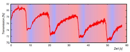
Figure 1B. A graph of light transmissivity over time, illustrating the BZ reaction (from Wikipedia DE)
What you are looking at is the Belousov-Zhabotinsky (BZ) reaction in a stirred beaker. It is striking in that the beaker’s liquid contents oscillate between a dark blue colour and clear transparency, for multiple cycles. Most of us can recall school chemistry lessons from the (more or less) distant past, where we saw reactions such as the titration of potassium permanganate with hydrogen peroxide, causing a beaker or tube full of liquid to change from dark purple color to clear, or vice versa. But not many of us probably saw the oscillating BZ reaction with a tube of liquid oscillating between the two starkly contrasting states. The BZ reaction “involves several reagents and various intermediate species; the central reaction step is the oxidation of malonic acid by bromate, catalyzed by metal ions” (Matthias Bertram 2002). The system is jumping between two states looking for equilibrium but finding it in neither.
This is intriguing to watch but what is going on here, and what significance does it have to climate, to the behavior of atmospheres and oceans?
The BZ reaction is a gateway to a whole branch of science which is, to repeat, still very incompletely explored and whose significance is under-appreciated. The two individuals, Boris Belousov and Anatol Zhabotinsky, who established their eponymous reaction, have an interesting history which has some resonance with the politics of climate science. Boris Belousov accidentally came across the oscillating reaction in Soviet Russia during the early 1950’s (one of the important and long undiscovered Soviet scientific discoveries that also included the “Ilissarov frame” orthopedic method for making new bone by gradual movement apart of fractured bone ends). Belousov’s attempts to publish this finding were rejected repeatedly, on the grounds of the familiar “where’s the mechanism?” argumentum ad ignorantium. In 1961 a graduate student Anatol Zhabotinsky took up and ran with the discovery, but it was not until an international conference in Prague in 1969 that the reaction became widely known, two decades after its inception.
The BZ reaction is a “reaction-diffusion system”. It is a non-equilibrium pattern phenomenon known as a nonlinear oscillator; there are certain prerequisites for such a system to develop:
- The system is far from equilibrium
- It is an open system with a flow through of energy (dissipative)
- The system has an “excitable” medium
The BZ reaction meets these requirements sufficiently to set off nonlinear oscillation. Note that condition 2 is only partly and temporarily met – a tube of chemicals is not really open; however the availability of reagents makes the system for a limited time behave like an open system until the reagents become exhausted.
The BZ reaction in a thin film
There are many types and flavours of the BZ reaction. In the first example we saw the reaction in a beaker: however when the reaction is carried out in a thin film, a new element arises: instead of the solution changing colour en-masse, the colour changes are associated with intricate evolving patterns such as radiating ripples and spirals.
You can search for “BZ reaction” on youtube and find many examples of attractive moving patterns, some with musical accompaniment. One of these is given in the link below:
Figure 2. Three animations of the BZ reaction in a thin film, showing evolving spatiotemporal waves and patterns and alternations of dominant colour phase.
This link presents three BZ thin film animations. In the first, regions of orange and pale blue colour repeatedly expand and contract, encroaching on each-other reciprocally, such that looking at the dish as a whole, the predominant colour alternates between orange and pale blue. The second animation is one where typical BZ fringe and spiral patterns in dark and light purple radiate from various centers. If you look in the bottom left corner, a tongue of darker purple periodically grows and recedes. The third animation is a slower moving version of the first – if you have the patience to watch all of it, again there is an overall pattern of alternation between orange and pale blue as the predominant colour.
Another youtube video of a thin film BZ reaction is given in the link below; while it is tediously slow and would have benefited from acceleration, it shows nicely the radiating BZ patterns characterized by alternation between orange and pale blue as the predominant color.
http://www.youtube.com/watch?v=S20Jsfu9rkQ
Figure 3. Another animation of the BZ reaction in a thin film showing travelling patterns and alternating phases.
During some parts of these BZ sequences, especially of the first animation, you have the feeling that you could be watching one of Bob Tisdale’s animations of the temporal evolution of sea surface temperatures (SSTs), such as that occurring in the equatorial Pacific with alternating el Nino and La Nina cycles: such an animation is given (By Bob) in the link below:

Figure 4. An animation of sea surface temperature anomalies in the Pacific during the transition from el Nino to La Nina systems during 1997 – 1999 (from Bob Tisdale’s blogspot), from web page: http://bobtisdale.blogspot.com/2010/12/enso-related-variations-in-kuroshio.html
If one focuses on the south eastern Pacific off the Peruvian coast, where the alternating tongues of warm and cool surface water characterize respectively the alternating en Nino and La Nina, the analogy to the BZ reaction is particularly compelling.
The ENSO as a nonlinear oscillator?
However beyond an intriguing qualitative visual similarity, what basis is there for proposing that the ENSO could constitute the same type of nonlinear oscillator as the BZ reaction? Please note that I am not proposing that chemical reactions play a role in the ENSO – no, chemical potentials in the BZ reactor are matched by thermodynamic potentials in the atmosphere-ocean system. Specifically we can return to the question of the essential pre-requisites that the BZ system meets to operate as a nonlinear oscillator; how would the ENSO system also meet these pre-requisites?
1. A system far from equilibrium
At least this one is a no-brainer. Solar energy input is very unequally distributed on the earth’s surface, maximally at the equator and minimally at the poles. Add to this the rotation of the earth and associated day-night cycle, and oblique axis rotation causing reciprocal summer and winter in north and south hemispheres, and ocean circulation, and it soon becomes clear that equilibrium is never remotely approached. (In fact, a world with atmosphere, ocean and heat flux in equilibrium is a nightmare to contemplate, with stagnant anoxic seas and stale motionless air.)
2. An open, dissipative system
The global climate system is open, as it receives heat input from the sun which (Leif Svalgaard notwithstanding ) is subject to minor periodic fluctuation. Heat is also radiated out to space. Heat energy enters and leaves the system; thus it is dissipative.
3. A system with an excitable medium
This is perhaps the most critical requirement. “Excitable” implies that an induced change at one location sets in motion a positive feedback which results in local amplification and propagation of the induced change – for instance taking the form of a travelling wave in the BZ reaction. This is not a wave in the sense of an energy wave through water or air that merely transmits energy, but a wave in which a spreading reaction is stimulated generating new local energy with the propagating wave. A cascade of chemical reactions in the BZ reaction constitutes this excitability. This positive feedback is limited and runs its course – characterised by a refractory period – but its operation is sufficient to drive and sustain the nonlinear oscillation, and in some cases to generate complex spatiotemporal patterns.
How could such excitability exist in the equatorial Pacific where the ENSO takes place? To discuss this question I need to refer to an exchange I had a few months ago with Bob Tisdale on a thread here at WUWT. The topic was one of these chicken-and-egg discussions of what drives the ENSO, either top-down by trade winds for instance, or bottom up by variation in deep upwelling. I posed the question to (who better?) Bob Tisdale, suggesting that the spread of both the el Nino and the La Nina, could involve a time-limited positive feedback. The nature of these positive feedbacks is indicated in the two diagrams below.

Figure 5. The La Nina positive feedback: enhanced Peruvian cold upwelling sharpens the equatorial Pacific east-west pressure gradient, driving stronger trade winds which propel further upwelling.

Figure 6. The el Nino positive feedback: decreased upwelling weakens the trade winds which propel the upwelling.
Please note that in the schematic systems in figures 5 and 6 it is not really relevant which comes first – changes in the trade winds or in upwelling. They are linked in a feedback loop. The analogy that I had in mind was of the on-shore and off-shore breezes that occur in summer in temperate coastal locations such as the British Isles. Here, in the day, increasing land temperature warms the surface air, causing it to decrease in density and rise, drawing in on-shore winds from the sea. Conversely at night, the land temperature quickly cools, increasing surface air density such that the wind is reversed to an off-shore breeze. (By contrast the air temperature over the sea is relatively constant). It was this essential mechanism that I suggested for the equatorial Pacific ENSO system, that the upwelling off Peru associated with the start of a La Nina cycle, in cooling the east Pacific surface layer air, creates a higher air pressure or density to the east that acts to drive east-to-west (easterly) trade winds (of the type that propelled Thor Heyerdahl and his companions on their epic Peru to Indonesia crossing of the Pacific on their “Kon Tiki” balsa wood raft, recapitulating the voyages millennia earlier of Polynesian mariners and ocean island settlers). These energised trade winds will push Pacific surface equatorial water westwards, adding impetus to the Peruvian upwelling by drawing eastern Pacific deep water toward the surface in a conveyer-belt like fashion. Thus the full cycle of a positive feedback illustrated in figure 5.
Conversely, during an el Nino cycle, upwelling is slowed or interrupted, resulting proximally in increased solar heating of more static, less mixed surface water in the Pacific east. This will decrease the temperature and pressure east-west difference, sapping force from the trades and resulting in doldrum conditions of decreased winds. The weakened trades will then slow the upwelling conveyor, connecting a feedback cycle that moves toward interrupted upwelling and a rapid spread of warm surface water from the east Pacific (figure 6).
It was a big moment for me when Bob Tisdale replied to the affirmative, agreeing that a time-limited positive feedback did indeed drive the onset of el Nino and La Nina, until both ran their course, reaching, to quote the term Bob used, “saturation”. Of course the whole system involves more complexity than this idealised system – there are periods of neither el Nino nor La Nina, or of modified, “Modoki” el Nino systems. However for me Bob’s positive reply was very important because the final piece of the jigsaw for this BZ-reaction analogy fell into place. Now I had my excitable or reactive medium. So it began to become clearer that the ENSO can indeed be characterised as a nonlinear oscillator, analogous to the BZ reaction-diffusion system.
3. The attractors and longer term pattern of ENSO (the PDO)
A feature of non-equilibrium pattern systems and their spatio-temporal evolution is an attractor. An attractor is a subset of the (often multidimensional) phase space that characterises a system, towards which the evolving system state converges. When an attractor takes on a complex fractal form it becomes a “strange attractor”. The strangeness of attractors does not however mean that they are not well understood – on the contrary, many different classes of attractor have been identified and studied mathematically.
A somewhat dry and technical description of attractors is given in wikipedia:
http://en.wikipedia.org/wiki/Attractor
In the context of our analogy of the ENSO as a nonlinear oscillator, a particularly interesting type of nonlinear attractor is the Lorenz attractor. Figure 7 below shows the time plot of phase space displacement of a Roessler and a Lorenz attractor. In figure 8, the phase space trajectory plot is given for the two corresponding attractors. The Lorenz attractor displays phase space “tearing” into two separate domains, while the Roessler attractor is characterised by phase space folding. The bilaterally torn attractor is sometimes referred to as the Lorenz “butterfly”.
(The chaos butterfly is rehabilitated! Providing one understands that one is referring to the Lorenz butterfly attractor, not the spurious “butterfly wing” effect.)
Of course, the Lorenz and Roessler attractors are simple classic types of nonlinear attractor. The Lorenz attractor exhibits oscillation of a fractal nature on more than one scale: the fine scale oscillation itself oscillates over a longer time period between higher and lower values of the phase space parameter on the y axis. More complex versions of both attractors exist – and many further types also. Figure 9 shows two examples, a Roessler attractor which shows tearing like a Lorenz attractor, and a folded chaotic BZ reactor attractor which kind of looks like a cross between a Roessler and a Lorenz.
 Figure 7. The time plot of phase space displacement of a Roessler and a Lorenz attractor.

Figure 8A. The phase space trajectory plot of the Roessler attractor (folding)
 Figure 8B the Lorenz attractor (tearing).
 Figure 9A. A half inverted torn chaos solution to a Roessler attractor
 Figure 9B. a folded chaotic BZ attractor.
A note on reading the literature on chaos and non-equilibrium pattern dynamics. Only pay minimal attention to the text and even less to the maths. Just look at the pictures. It is the spatiotemporal multidimensional patterns that are the unifying and compelling feature, and it is pattern analogies between disparate systems which reveal the unifying pattern processes at work. In the above figures I have not defined the parameters in the x and y axis – they don’t really matter.
The Lorenz attractor and the ENSO
Does the time plot of the Lorenz attractor in figure 7 (b), with its higher and lower frequency components, remind you of anything? The wavetrain appears to spend alternating periods oscillating in a higher and a lower region of the y axis. Here again our discussion turns to the definitive work by Bob Tisdale on the ENSO. Bob’s recent posting on WUWT (reposted from his own blogspot) entitled “Integrating ENSO: multidecadal changes in sea surface temperature” had the subtitle “Do multidecadal changes in the strength and frequency of el Nino and La Nina events cause global sea surface temperature anomalies to rise and fall over multidecadal periods?”. A link to this article (pdf) is:
This tour-de-force of the ENSO and its controlling influence on global SSTs demonstrated how, over the past century, there have been alternating periods of about three decades duration during which the el Nino and La Nina systems are reciprocally dominant. Two plots from Bob’s article are shown below in figure 10.
Figure 10a shows the ENSO oscillations exhibiting alternating periods of higher and lower elevation on the y axis (Nino SST 3.4 anomalies), although with far more noise than the tidier level-switching oscillation of the Lorenz attractor. The Nino 3.4 plot thus resembles a very untidy or chaotic Lorenz attractor time plot of the type shown in figure 7b. The alternating periods dominated by the el Nino (1910-1944, 1976-2009) and by La Nina (1945-1975) represent the two wings of the Lorenz butterfly. Thus this period-alternation between a generally warming el Nino dominated phase and a cooling La Nina dominated phase, fits in with the description of the ENSO system as a nonlinear oscillator, of the BZ reaction type, and characterised by a torn attractor of the Lorenz – or possibly modified torn Roessler – variety. It is also known as the Pacific decadal oscillation, or PDO.

Figure 10A. The Nino 3.4 SST anomalies from 1910 to the present, averaged into roughly 30 year periods by Bob Tisdale.

Figure 10B. Global SST compared to period-averaged Nino 3.4 anomaly. Both from “Multidecadal changes in sea surface temperature” by Bob Tisdale.
Is the PDO the Lorenz butterfly attractor of the ENSO?
Closely linked to the ENSO is the PDO – indeed Bob Tisdale asserts that the PDO is an epiphenomenon of the ENSO. His recent posting on multidecadal variation in SSTs elucidates this relationship, showing the PDO to essentially comprise alternating periods of el Nino and La Nina dominance. On the basis of the proposal presented here that the ENSO is a nonlinear oscillator, we can suggest further that the alternating “PDO” phases are the paired “butterfly wings” of a Lorenz attractor characterising the ENSO.

Figure 11. Could the Pacific Decadal Oscillation (PDO) represent the operation of a Lorenz “butterfly” torn attractor on the ENSO?
Periodic forcing of the ENSO nonlinear oscillator
At this point, some of you may be saying “hold on a moment – I’m not convinced by this BZ reaction analogy. Most of the BZ reactions (e.g. shown on youtube) show spiral and fringe patterns that are not at all persuasive analogies to the shifting regional patterns of ocean surface temperatures”. You would have a point. However it is necessary at this stage to introduce another class of nonlinear oscillators – the periodically forced nonlinear oscillator. The BZ reactions that were referred to above, and shown in the attached movies, are all unforced examples. These unforced BZ reactions oscillate and their own natural frequency, and are indeed often characterised by such radiating spiral and fringe patterns. But the spatiotemporal patterns can change profoundly when the BZ reaction is subject to periodic forcing. Figure 12, provided by Matthias Bertram’s PhD thesis, shows a series of spatial patterns from a BZ reaction which is catalysed by a light sensitive metal catalyst, then subject to various regimes of periodic forcing by light pulses. The first case (a) is unforced and looks like many of the youtube BZ reaction animations. However a wide range of different patterns is observed (b-g) when different periodic forcings are applied.

Figure 12. A BZ reaction with a light-sensitive metal catalyst, showing spatially extended nonlinear oscillator patterns. Case (a) is unforced; all the remaining are subject to different amplitudes and frequencies of light pulse periodic forcing. Taken from the PhD thesis of Matthias Bertram.
Anna Lin et al. (2004) looked further at the role of periodic forcing in the light-sensitive BZ reaction. The BZ system in the absence of forcing oscillates at its natural frequency. When forcing was applied by periodic light flashes, they found a difference in the kind of response depending on whether the forcing was strong or weak. To quote the authors:
“The entrainment to the forcing can take place even when the oscillator is detuned from an exact resonance [refs]. In this case, a periodic force with a frequency f(f) shifts the oscillator from its natural frequency, f(0), to a new frequency, f(r), such that f(f) / f(r) is a rational number m:n. When the forcing amplitude is too weak this frequency adjustment or locking does not occur; the ratio f(f) / f(r) is irrational and the oscillations are quasi-periodic. In dissipative systems frequency locking is the major signature of resonant response.”
So with strong forcing, “frequency locking” occurs and there is a clear relationship between the frequencies of the periodic forcing and of the BZ systems responsive forced oscillation. However when the forcing is weak, the reaction’s responsive frequency shows a much more complex relation to the forcing frequency, and its resultant oscillations can be described as “quasi-periodic”.
Returning to the ENSO, how could the equatorial Pacific nonlinear oscillator be periodically forced? Periodic forcing of the oceans and of climate in general is a frequent topic of posts at WUWT. There are many such known and potential sources of periodic forcing over a wide range of time-scales. The Milankovich orbital related cycles operate over periods of 105 years to decades and centuries (in the case of resonant harmonics of orbital oscillations). Then there is oscillation in solar output from the 11 year sunspot cycles to the longer periodicities such as the Gleissburg cycles. One persuasive source of PDO forcing is solar-barycentric, as outlined by Sidorenko et al. (2010), the movement of the solar system barycenter around the sub-Jupiter point (center of gravity of a solar system containing only the sun and Jupiter):
This periodic asymmetry in the solar orbit has shown a wavelength and inflection points similar to the PDO cycle in the last two centuries.
Turning to the oceans and the thermo-haline circulation of deep ocean currents, it is well known that the strength of cold water downwelling at the key sites such as the Norwegian sea is subject to significant variation – indeed after a period of a few decades of relative weakness, Norwegian sea downwelling has recently strengthened (Nature, 29 November 2008, doi:10.1038/news.2008.1262 – link in references). Once could go on. There is no shortage of potential sources of periodic forcing of the atmosphere-ocean system, either of the equatorial Pacific or indeed globally.
If the PDO represents the operation of the ENSO Lorenz attractor, then the periodicity of the PDO should tell us if the system is unforced or forced and frequency locked – in which cases it would have regular periodicity, or if it is weakly periodically forced, in which case an irregular wavelength might be expected. Jacoby et al. 2004 traced the PDO oscillations over the last 400 years, using oak tree rings on the Russian Kurille Islands:
http://www.wsl.ch/info/mitarbeitende//frank/publications_EN/Jacoby_etal_PPP_2004.pdf
A PDO wavetrain is clearly discernible but the wavelength varies from 30-60 years. The PDO thus appears to be a real multidecadal oscillation but it is not frequency locked, showing frequency variation. This points to the PDO arising from a weakly periodically forced ENSO. Mantua et al. (2002) also review data on palaeo-records of the PDO, concluding that its wavelength varies from 50-70 years. They concluded that the causes of the PDO are unknown.
http://www.atmos.washington.edu/~mantua/REPORTS/PDO/JO%20Pacific%20Decadal%20Oscillation%20rev.pdf
Thus the PDO seems to be almost but not quite regular – apparently aiming for a 60 year cycle but fluctuating from it. This could be evidence of periodic forcing of the ENSO system that close to the boundary between “weak” and “strong” forcing. Of course, these suggestions about sources of periodic forcing of the ENSO and PDO are speculative. If, as set out by Lin et al. (2004), in the case of a weak periodic forcing of a nonlinear oscillator such as the BZ reactor, the relation between a putative forcing frequency f(f) and the responsive frequency f(r) is irrational, this complicates the search for conclusive proof of such a link. However the PDO’s apparently limited departure from 60 year periodicity might suggest a forcing near the boundary of strong and weak, and therefore an intermittent frequency locking.
Conclusions
- Owing to the far-from-equilibrium state of the earth’s atmosphere and ocean climate system, the a priori case for the operation of non-equilibrium/nonlinear pattern dynamics is strong.
- The Belousov-Zhabotinsky reaction-diffusion system in a thin film is a compelling model of a nonlinear oscillation arising spontaneously in a far-from-equilibrium spatially-extended system, with apparent similarities to the ENSO sea surface temperature spatio-temporal oscillation in the equatorial Pacific.
- The apparent positive feedbacks (spatio-temporally limited) associated with the initiation of both el Nino and La Nina systems, linking Peruvian coast deep upwelling with equatorial trade winds, qualify the equatorial Pacific as an excitable medium, a key pre-requisite of an oscillating reaction-diffusion system such as the BZ reaction. The open and dissipative nature of the climate and ocean meet another such requirement.
- Of the class of known attractors of nonlinear oscillatory systems, the Lorenz and possibly Roessler attractors bear similarities to the attractor likely responsible for the alternating phases of La Nina and el Nino dominance that characterise the ENSO and constitute the PDO.
- It is possible that the ENSO / PDO system might be periodically forced; the significant but limited variation of the time-period of the PDO evidenced in the palaeo-record of the last few centuries suggests a forcing strength close to the threshold required for frequency locking.
- If the ENSO and PDO can be characterised as a nonlinear oscillator with a Lorenz type attractor, one might speculatively extend the analogy more widely to the earth’s climate as a whole, and such features as the alternation between glacial and interglacial states (during a glacial epoch such as the present one).
- It is hoped that scientists and mathematicians with expertise in non-equilibrium pattern systems, such as reaction-diffusion oscillatory systems, might bring their analytical techniques to bear on the study of the earth’s atmosphere, oceans and climate. In this way the hypotheses presented here could be confirmed or refuted, and perhaps the nature and identity of the significant drivers of climate could be found.
Postscript
What implications does this paper have for anthropogenic global warming (AGW), if any? It was not written primarily to address the AGW issue. CO2 is not mentioned. However there are some indirect implications. The finding that Bob Tisdale’s observation of alternating periods of el Nino and La Nina dominance – in other words the PDO – is well described by a nonlinear oscillator driven by a torn Lorenz (or Lorenz-Roessler) attractor, give Bob’s conclusions greater “real-world” plausibility. (Nonlinear attractors are a common feature of the real world.) It is also a riposte to those who argue against the reality of the PDO or AMO (Pacific decadal oscillation, Atlantic multidecadal oscillation) on the grounds that a credible mechanism does not exist. It does!
One important mathematical aspect of a nonlinear oscillator with an attractor is its “Lyapunov stability”. Alexander Lyapunov, from Yaroslavl, Russia, established a century ago the maths of stability of both linear and nonlinear systems, such that a nonlinear system such as an oscillator is characterised by a “Lyapunov exponent”. The full works on this are given here:
http://cobweb.ecn.purdue.edu/~zak/ECE_675/Lyapunov_tutorial.pdf
The maths here is all way over my head – I’m a “mere” biologist! Essentially the Lyapunov exponent assesses how strong or “attractive” the attractor is – i.e. how strong a perturbation of the system is needed to move it – unwillingly – away from its attractor. More expert mathematic analysis of the ENSO as nonlinear oscillator would include derivation of the Lyapunov exponents. This would tell us the stability of the system and its resistance to change due to any outside influences.
The global circulation models (GCMs) are essentially linear. That presumably is why they generally fail to reproduce the ENSO and PDO. (If they show any nonlinear behaviour it is probably more by accident than design.) It remains to be seen whether climate and ocean modelling – of the ENSO or of larger parts of the global climate, which used a nonlinear oscillator as a starting point, would be more effective.
Post-postscript
Mathematical / computer modelling of a nonlinear oscillator such as the BZ reaction is not too difficult (for people into that kind of thing) and well established. The “Brusselator” – so named for being invented at the Free University of Brussels (VUB) is a good example:
http://en.wikipedia.org/wiki/Brusselator
References
Controlling turbulence and pattern formation in chemical reactions. Matthias Bertram, PhD thesis, Berlin, 2002. https://docs.google.com/leaf?id=0B9p_cojT-pflY2Y2MmZmMWQtOWQ0Mi00MzJkLTkyYmQtMWQ5Y2ExOTQ3ZDdm&hl=en_GB
G. Nicolis and I. Prigogine, Self-organization in Nonequilibrium Systems (Wiley, New York, 1977).
E. Schroedinger, What is Life ? (Cambridge Univ. Press, 1944).
P. Glandsdorff and I. Prigogine, Thermodynamic Theory of Structure, Stability and Fluctuations (Wiley, New York, 1971).
The ENSO-Related Variations In Kuroshio-Oyashio Extension (KOE) SST Anomalies And Their Impact On Northern Hemisphere Temperatures. Bo Tisdale, from the web page: http://bobtisdale.blogspot.com/2010/12/enso-related-variations-in-kuroshio.html
Integrating ENSO: Mutidecadal variation in sea surface temperature. Bob Tisdale.
Pdf of this article: https://docs.google.com/leaf?id=0B9p_cojT-pflYjYyMTdkYzItMDMwOS00MjFjLWJmYTAtMzdjYjM1YjhhMmFj&hl=en_GB
Resonance tongues and patterns in periodically forced reaction-diffusion systems. Anna Lin et al., DOI: 10.1103/PhysRevE.69.066217, Cite as: arXiv:nlin/0401031v1 [nlin.PS].
Nature, 29 November 2008, doi:10.1038/news.2008.1262.
http://www.nature.com/news/2008/081129/full/news.2008.1262.html
G. Jacoby, O. Solomina,1, D. Frank, N. Eremenko, R. D’Arrigo (2004) Kunashir (Kuriles) Oak 400-year reconstruction of temperature and relation to the Pacific Decadal Oscillation. Palaeogeography, Palaeoclimatology, Palaeoecology 209 (2004) 303–311.
http://www.wsl.ch/info/mitarbeitende//frank/publications_EN/Jacoby_etal_PPP_2004.pdf
Mantua et al. (2002)
http://www.atmos.washington.edu/~mantua/REPORTS/PDO/JO%20Pacific%20Decadal%20Oscillation%20rev.pdf
N. Sidorenkov I.R.G. Wilson A.I. Kchlystov (2010) Synchronizations of the geophysical processes and asymmetries in the solar motion about the Solar System’s barycentre. EPSC Abstracts Vol. 5, EPSC2010-21, 2010 European Planetary Science Congress 2010.
I’m not very good with names but a russian scientist discovered this oscillante/pattern process accidently and was (as usual) laughed out of court. He finally committed suicide. It was during the cold war so the info never got out. Turin kicked it off through his study of animal skin patterning eg Giraffe and Zebra. Turin actually defined some equations which when run in a computer showed the same oscillante patterns. He too was eventually driven to suicide and this work died with him. The russian and Turin were of the same era but never knew of each other’s work.
Re: jtom says:
January 25, 2011 at 6:53 am
“Please keep all researchers and scientists away from the Peruvian coast – not a good place for large-scale experimentation! I’d hate for someone to drop a few hundred tons of salt into the ocean off of the Peruvian coast to see what would happen!”
If you’d ever been involved in a really big, government funded, large-scale experiment, you wouldn’t worry about this one. By the time they’d overrun their entire budget several times over, you might find one lonely dump-truck load of salt sitting on the Peruvian beach, but none in the ocean. The combined weight of the attendant, published research papers would outweigh that forlorn little pile of salt.
APACHEWHOKNOWS sorry, but the handle reminds me of another way to forecast climate:
It’s late fall and the Indians on a remote reservation in South Dakota asked their new chief if the coming winter was going to be cold or mild.
Since he was a chief in a modern society, he had never been taught the old secrets. When he looked at the sky, he couldn’t tell what the winter was going to be like.
Nevertheless, to be on the safe side, he told his tribe that the winter was indeed going to be cold and that the members of the village should collect firewood to be prepared.
But, being a practical leader, after several days, he got an idea. He went to the phone booth, called the National Weather Service and asked, ‘Is the coming winter going to be cold?’
‘It looks like this winter is going to be quite cold,’ the meteorologist at the weather service responded.
So the chief went back to his people and told them to collect even more firewood in order to be prepared.
A week later, he called the National Weather Service again. ‘Does it still look like it is going to be a very cold winter?’
‘Yes,’ the man at National Weather Service again replied, ‘it’s going to be a very cold winter.’
The chief again went back to his people and ordered them to collect every scrap of firewood they could find.
Two weeks later, the chief called the National Weather Service again. ‘Are you absolutely sure that the winter is going to be very cold?’
‘Absolutely,’ the man replied. ‘It’s looking more and more like it is going to be one of the coldest winters we’ve ever seen.’
‘How can you be so sure?’ the chief asked.
The weatherman replied, ‘The Indians are collecting a shitload of firewood’
I think that to invoke chaos might be just the same as giving up,it is just chaos.the patterns of enso/pdo are interesting and it will be important to see how they develop with world temperatures in the coming years with regard to co2 concentration in the atmosphere and solar activity.
Bravo Antony. That’s exactly along the lines I was suggesting
In the global circulation patterns you will find the greatest strange attractor to be the Moon and its combination of tidal forces felt on the Earth, from the further modulation of solar electromagnetic effects, by the tidal and gravitational inner actions of the inner planets, at a period known as the Saros cycle of 18.03 years. (minus 27.3 days to get an even number [240] of cycles of the 27.3 day pattern of the magnetic rotation of the sun that drives the moon’s declinational position on the ecliptic in sync.)
IF you take three past cycles of this period and over lay the effects on the global circulation you will see three repeating patterns that are about ~80% predictive of the conditions of the next cycle. Which I think shows there is a predictable effect of the repeating drivers of the ocean oscillations, once you realize it is the moon, and look at the forces at work, watch animations of the GOES satellites showing the passage of the moon over lines of thunderstorms, surges in growth in hurricane intensity, most noticeable in their early formations.
In fact I have taken the past weather data for the USA and presented the composite maps as forecasts for the past three years and the next three years. The forecast for today [generated with a three year lead time], looks about like the daily total composite radar.
IF this cyclic repeating pattern of weather can forecast the next cycle (Today) now can you not think that there is something else than CO2 to look at? Lot more details in the research section of the site.
Murray Duffin says:
January 25, 2011 at 10:33 am
One more point – turn Fig 1B upside down and it is reminiscent of the last several 100k years of glacial/interglacial oscillations.
My thoughts exactly! Interesting times we live in.
I have a question about the ENSO cycle that is fueled by thinking about the recent post on the trends of the last 10-12 years, but that thread is exhausted so I’ll post the question here, and hope it’s meaningful.
My understanding of the ENSO cycle is that in many respects the underlying physics is the opposite of what seems to be the case. In other words, during a La Nina event, although the surface ocean temps cool dramatically and this leads to cooling of global atmospheric temperatures, what is actually going on is that the tropical sun is warming the surface waters and evaporating them, leading to higher saline content and a sinking of these warmer yet heavier waters into a subsurface zone that stays there for years. So the La Nina event is actually a “warming event”, from the ocean’s point of view, even if it appears to be cooling event.
Likewise, the El Nino warming events are actually a cooling process from the ocean’s point of view, in that the warmer, sunken heat from the La Nina event finally surfaces and produces higher than normal surface temps which then heat up the atmosphere until the heat is finally dissipated. Hence, the atmospheric warming is actually part of a cooling event, and this cycle then leads back to another La Nina event that produces cooling of the atmosphere, but warming of the ocean beneath the surface.
So my question is about how this process works over many cycles to either warm or cool the general climate. I’m curious as to whether the huge 1998 El Nino was as much responsible for the climate moving to a higher temperature level as the longer La Nina event that followed it. And also, if in some respects it would lower temps for the La Nina events to become less powerful or at least shorter in duration, so that less heat becomes stored in the sub-surface ocean to emerge later as a surface warming event.
Basically, I’m asking for more detail on how this system actually works during a general climate cooling cycle. Some say that stronger La Nina events will lead to a cooling climate, but shouldn’t the opposite be the case in the long run? I guess I’m a little confused as to how this works, and what to look for as a sign of a cooling climate cycle ahead.
Maybe we should be using some kind of speech recognition software to find out what language nature is using and what she is trying to tell us. Our present climate models are not Rosetta stones.
Great article!
I just hope this doesn’t drag too many dancing off into never land. I have never viewed the earth’s climate system as chaotic. Now “infinitely complex”, that I buy. Chaos as I read has no limits but this world has all kinds of limits, it is limited by diffusibility, thermal conductivity, inertia, momentum, acceleration, specific heats, and on and on and on. But can you see very similar effects within the climate, absolutely. The visuals in this article are fantastic.
But I have to still to feel that what we see is hundreds of coupled equations of cause and effect, many times interconnected and recursive across three or more cause and effect links and all having limits placed on them by physics, the physical limits, to how fast they can proceed in reality and these loops within the graph (mathematical graph that is with nodes and links) that makes it appear chaotic with endless patterns. That’s just my view.
I have to say though that mathematics in the realm of chaos may very well give us the best approximations that mimic these processes and should be pursued. It may be the only real way we can even approach a mathematical solution for in reality it is simply too complex for computers today, we can only approximate.
But still, this was a great article Phil. Opens your mind.
In the discussion about forcing and whether or not the period was weakly or strongly locked there was an implicit assumption that the forcing was periodic. However it not impossible (and indeed quite likely) that the forcing itself is only weakly periodic. The world weather system is probably best described as a series of linked chaotic oscillators.
Good stuff. Will need some time to digest.
polistra says: January 25, 2011 at 6:36 am “There’s a much less obscure example of a nonlinear oscillator, much easier to observe and experiment on. The human heart. ”
For some years I’ve had a mental image of climate fluctuations not just as a heart, but as a body, which has other repetitive cycles such as respiration. Each can, in theory, be varied independent of the other, but OTOH some factors like exertion can cause both to change together. Then there are other variables like adrenalin production, the ATP cycle .. probably the list is long. The difficulty is to isolate the behaviour of one pulsating element from the confounding effects of the others, which can sometimes give the appearance of a resonance (hence records get set).
The BZ example with changing colours remins me of two effects, which we can use here by example of easy things for chemists, being pH and oxidation state. I’m not at all saying these are the actuals, just examples. Both pH and degree of oxidation can be changed (in theory) independently. Both can change the colour of solutions. But they can also act together. When they act together, I think of the predator-prey mathematics, which in some circumstances might tip a happy pH out and put in a happy oxidation state. Then vice versa. Hence the oscillation.
This is a verbal description to help understand the way things appear. I do not pretend that it is verifiable by easy mathematics.
Another topic above is self-replication. There is a lovely example from nature, the “broc-cauli” or Brassica romanesque. The whole resembles the shape of its parts, which are placed in a non-random order. The parts of a sub-part resemble a sub-part, and so on until botanical noise takes over and the detail is lost.
It’s worth a look at http://en.wikipedia.org/wiki/Romanesco_broccoli
I sometimes think not all La Ninas are true La Ninas but merely a cooling of the tropical pacific waters following an El Nino event.
The graphic above of the 1998-9 La Nina(Fig 4) shows the tropical waters cooling FROM the WEST.
The current La Nina emerged from the EAST and travelled WEST as we’d expect would happen with cool upwelling waters along the Peruvian coast.
The current La Nina is also accompanied by much cooler sub-surface waters, up to 4DegC according to the Oz BoM
Looking at the sea level chart on the WUWT ENSO page the 98-9 La Nina associated sea level drop wasn’t exceptional, the lower limit was still higher than the 1997 lower limit.
However, the current sea level drop associated with this La Nina is more substantial and still dropping.
These lead me to believe that not all La Ninas are true La Ninas even though the indices may suggest they are.
There’ll be a clue in the changing lengths of the PDO cycle from around 30-60 years, and the distribution of Los Ninos and Las Ninas therein, with the sun somehow forcing, whether it be magnetically, electrically, with albedo functions or with cosmic rays or Erl’s sultry ultryviolet ones. I still think the stability of these two flipped phenomena must ameliorate the hypersensitivity which might accrue from whatever solar mechanisms are most active.
=========
This is a nice, graphical layman’s introduction to the labyrinth of nonlinear, equilibrium-seeking systems. The idea of ENSO as a nolinear oscillator, of course, has been bandied about for many years. What makes ENSO so fascinating, however, is that the idea does not pan out dynamically without specifying a forcing of the subdecadal oscillations that persistently characterize the phenomenon, which is a leading indicator for global temperatures in that spectral range. What really drives ENSO thus is as much a mystery at present (up through Dijkstra’s 2005 monograph) as ever.
It is far easier to determine what does NOT. Certainly Milankovitch cycles, measured in tens of thousands of years, can be ruled out; thousand-order harmonics make no sense on physical grounds. Thermodynamics at terrestrial temperatures has not demonstrated any resonance, eliminating strong subharmonics from consideration. The multidecadal signal components of ENSO3.4 are, at any rate, minor in magnitude and virtually incoherent with global temperatures. Thermohaline circulation is not a factor in the iconic upwelling off the coast of Peru, which is driven by wind-stresses rather than density. And true positive feedback–as opposed to energy recirculation, with which it it often confused–runs afoul of Lyapunov stabilty. Thus we are left with speculation based on qualitative similarities of some features of time series, rather than with quantitative science.
Thank you all, I have read the article and the posts a couple of times. I will never understand the math but I like the questions and the fact that they lead to more questions which may increase our understanding of what is going on. I have a question to add. Does anyone understand the ocean circulation in three dimensions? I see a lot about gyres and connection with the winds. I see people talking about upwelling and down welling but I also know that the old “conveyor belt” theory was shown to be be misunderstood once neutral buoyancy floats were used to track the deep currents and they were found to be diffuse (ignoring the complexity and probable errors in the tracking system). Basically I see a lot of assumptions being made as you can’t start off from first principles. You need a starting point to create a hypothesis, but how do you know the hypothesis is correct? We are learning that so much of what were taught in University and in business was based on flawed research. Yet things worked. I recall feeling really good about getting 90% on one of my differential equation and vector analysis exams … until I thought about it and realized that if 10% of the bridges one of my fellow engineers designed fell down, this would not be good. Bridges need to stand up 100% of the time. (They don’t, but that is another story.)
It took me hours to read, re-read and think about the last few posts here.
A lot of good thoughts and I suspect in 30 or 40 years we will have a much better understanding of how our world works. In the mean time, we will keep applying reasonable safety factors to make sure those bridges you drive over stand up, even though we may not always know why.
A bientot.
Great article.
I got the impression that Mr. Watts is a little suspect of “chaos” as a branch of anything scientific, and I tend to agree. Chaos is an anthropomorphic construct
of a situation that we either are too stupid to understand or don’t have all the facts on, or both. I doubt that God ever uses the word.
“However beyond an intriguing qualitative visual similarity, what basis is there for proposing that the ENSO could constitute the same type of nonlinear oscillator as the BZ reaction?…”
Probably none.
It’s an interesting article.
It has crossed my mind that ENSO and other ocean “oscillations” might be chaotic. It has provably occurred to others.
However these assertions should be checked
———
1. The global circulation models (GCMs) are essentially linear.
2. That presumably is why they generally fail to reproduce the ENSO and PDO.
3. (If they show any nonlinear behaviour it is probably more by accident than design.)
I suspect they are not correct.
PaulM says:
January 25, 2011 at 7:28 am
The idea of the positive feedback loop that you describe is useful for demonstrating how an instability of the system might arise.
But it does not really explain the oscillations.
An interesting mechanism that generates oscillations is negative feedback, combined with a time delay.
Requires both negative and positive feedback with a time delay.
If you look at the annual rainfall for Sydney Australia, you will see a very chaotic pattern.
There are large spikes upwards every 20, 40 or 60 years or so.
In between the rainfall declines in a zigzag pattern.
The long term trend since 1859 has been flat (R squared 0.0001).
There are two basic chaotic patterns, according to Hurst.
Sydney rain is chaotic of the type – “mean reversion” as opposed to “random walking”.
That is typified by a generally spiky shape – one year up, the next down.
(Hurst number close to zero, on a zero to one scale, 0.5 being Brownian motion).
In Australia, annual maximum average temperature tends to vary with rainfall, except when boosted by UHI.
Sydney is a prime example.
stephen richards says:
January 25, 2011 at 11:43 am
I’m not very good with names but a russian scientist discovered this oscillante/pattern process accidently and was (as usual) laughed out of court. He finally committed suicide. It was during the cold war so the info never got out. Turin kicked it off through his study of animal skin patterning eg Giraffe and Zebra. Turin actually defined some equations which when run in a computer showed the same oscillante patterns. He too was eventually driven to suicide and this work died with him. The russian and Turin were of the same era but never knew of each other’s work.
That was Turing of course, Prigogine saw one of Turing’s lectures on the topic and it has been said that he owed his ’77 Nobel to Turing. Turing’s work didn’t die with him I teach his reaction-diffusion mechanisms in one of my classes for example.
Phil. says:
January 25, 2011 at 10:51 pm
PaulM says:
January 25, 2011 at 7:28 am
Nope, sorry.
http://www.electronics-tutorials.ws/oscillator/oscillators.html
Note that “in-phase” feedback with a plus is the same as “out of phase” feedback with a minus.
Mark