
Alternative title: “Standing on the shoulders of Giant Bob”
Guest post by Phil Salmon
Introduction
One of the themes to emerge from the climate debate here on WUWT, concerns “chaos” and nonlinear system dynamics and pattern. Anyone acquainted at all with the nature of dynamical chaos and nonlinear / non-equilibrium pattern formation, and who also has an interest in the scientific questions about climate, cannot fail to sense that dynamical chaos has to be an important player in climate. Simply on account of the huge complexity of climate over the expanse of earth’s surface and deep time, and also the obvious impossibility of equilibrium in a rotating system with continuous substantial imbalances of heat and kinetic energy.
However, a “sense” is hardly adequate scientifically; it is necessary to go further than this and forge some kind of physical and mathematical model or hypothesis which can be tested. But here one runs into the problem of chaotic systems being .. well, chaotic and unpredictable; indeed for some the movement of a system into the chaotic region represents falling off the edge of the world of scientific testability and orthodox Popperian experimental investigation. Is it a contradiction in terms to imagine that you can study chaos scientifically and mathematically? The scientific community at large – not only climate science – while giving lip service to chaotic pattern formation as a real phenomenon, generally shrinks back from serious engagement with it, back into the comfortable regions of tidy linear and equilibrium equations.
However there does exist a well-established science of physical and mathematical study of chaotic, nonlinear systems, in which a wide range of nonlinear pattern forming systems are well understood and characterized. But owing to the human tendency to associate in closed communities – nowhere more in evidence than in the multi-faceted scientific world, there is in my view too little engagement between the chaos and nonlinear dynamics experts and scientists in a wide range of natural sciences whose studied systems are – unknown to both sides – accurately and usefully characterized by well-researched nonlinear pattern systems.
It is the purpose of this article to propose a well-known experimental “nonlinear oscillator”, namely the Belousov-Zhabotinsky chemical reaction, as an analogy – in terms of its dynamics and spatio-temporal pattern – for the El Nino Southern Oscillation (ENSO) system in the equatorial Pacific Ocean. This would characterize and alternation between El Nino and La Nina as a nonlinear oscillator. The definitive work of Bob Tisdale on the ENSO is used to liken the alternating multi-decadal periods of eE Nino and La Nina dominance (the PDO) as the two wings of the Lorenz butterfly attractor.
The term “chaos”, while a common shorthand for a class of phenomena and systems, is not a very accurate or helpful one. Chaos itself, strictly speaking, is truly chaotic and not a very fruitful area of mathmatic investigation. A system passes from the region of linear dynamics through “fringes” or borderlands of mathematical bifurcation before reaching full blown chaos, and it is in these marginal and transitional borderlands where the interesting phenomena of strange attractors and spontaneous pattern formation arise. But it is hard to find a convenient single word that takes its place – it is easier to say “chaos” than “nonlinear pattern formation in far-from-equilibrium dissipative systems”.
Even “nonlinear”, while better than “chaos”, is still inadequate: there are plenty of physical and mathematical systems which are clearly not “linear” but not related to non-equilibrium emergent pattern formation. A relative of mine – a TV weatherman in Monterrey, California for many years before his retirement – pointed this out to me, that it is not necessary to invoke nonlinear pattern formation to account for acute sensitivity to initial conditions – a simple high power relationship is sufficient for this. Acute sensitivity to initial conditions does indeed characterize many nonlinear systems – indeed, one popular metaphor for chaotic systems is the “butterfly wing” effect – namely that a butterfly wing’s disturbance of the air in one place can result in massive changes in weather systems a continent away. The butterfly wing analogy was coined by Edward Lorenz – a pioneer in mathematical study of non-equilibrium pattern system and also a meteorologist – we will return to Lorenz later. However this sensitivity does not uniquely define the type of system we are considering. (The “butterfly wing” metaphor is now inseparable from the actor Jeff Goldblum and his rather inane use of the phrase in the Jurassic Park films.)
If I had to propose an alternative to “chaotic” as a general short term for such systems with spontaneous nonlinear pattern dynamics, I would go for something like “non-equilibrium pattern” systems.
One of the most helpful references I have found on the subject of non-equilibrium pattern systems is the PhD thesis of a chemical engineer Matthias Bertram, entitled “controlling turbulence and pattern formation in chemical reactions” – previously posted on his web site but now reposted on Google docs:
Matthias uses the term “pattern formation in dissipative systems”. To quote from the introduction of this thesis:
“The concepts of self-organization and dissipative structures go back to Schrodinger and Prigogine [1–3]. The spontaneous formation of spatio-temporal patterns can occur when a stationary state far from thermodynamic equilibrium is maintained through the dissipation of energy that is continuously fed into the system. While for closed systems the second law of thermodynamics requires relaxation to a state of maximal entropy, open systems are able to interchange matter and energy with their environment. By taking up energy of higher value (low entropy) and delivering energy of lower value (high entropy) they are able to export entropy, and thus to spontaneously develop structures characterized by a higher degree of order than present in the environment.”
The author goes on to analyze several experimental non-equilibrium pattern systems, including the Belousov-Zhabotinsky reaction. He outlines the essential conditions for the operation of a nonlinear oscillator such as a far from equilibrium state, and an “excitable medium”, that is, a medium within which localized positive feedbacks can be initiated and run their course according to their associated refractory period. We will return to these parameters when we consider the ENSO.
The Belousov-Zhabotinsky reaction
There is a helpful short introduction to the Belousov-Zhabotinsky (“BZ”) reaction on Wikipedia:
http://en.wikipedia.org/wiki/Belousov%E2%80%93Zhabotinsky_reaction

Have a look at this youtube video shown in figure 1:
Figure 1A. A video of the BZ nonlinear oscillation in a stirred beaker.
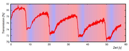
Figure 1B. A graph of light transmissivity over time, illustrating the BZ reaction (from Wikipedia DE)
What you are looking at is the Belousov-Zhabotinsky (BZ) reaction in a stirred beaker. It is striking in that the beaker’s liquid contents oscillate between a dark blue colour and clear transparency, for multiple cycles. Most of us can recall school chemistry lessons from the (more or less) distant past, where we saw reactions such as the titration of potassium permanganate with hydrogen peroxide, causing a beaker or tube full of liquid to change from dark purple color to clear, or vice versa. But not many of us probably saw the oscillating BZ reaction with a tube of liquid oscillating between the two starkly contrasting states. The BZ reaction “involves several reagents and various intermediate species; the central reaction step is the oxidation of malonic acid by bromate, catalyzed by metal ions” (Matthias Bertram 2002). The system is jumping between two states looking for equilibrium but finding it in neither.
This is intriguing to watch but what is going on here, and what significance does it have to climate, to the behavior of atmospheres and oceans?
The BZ reaction is a gateway to a whole branch of science which is, to repeat, still very incompletely explored and whose significance is under-appreciated. The two individuals, Boris Belousov and Anatol Zhabotinsky, who established their eponymous reaction, have an interesting history which has some resonance with the politics of climate science. Boris Belousov accidentally came across the oscillating reaction in Soviet Russia during the early 1950’s (one of the important and long undiscovered Soviet scientific discoveries that also included the “Ilissarov frame” orthopedic method for making new bone by gradual movement apart of fractured bone ends). Belousov’s attempts to publish this finding were rejected repeatedly, on the grounds of the familiar “where’s the mechanism?” argumentum ad ignorantium. In 1961 a graduate student Anatol Zhabotinsky took up and ran with the discovery, but it was not until an international conference in Prague in 1969 that the reaction became widely known, two decades after its inception.
The BZ reaction is a “reaction-diffusion system”. It is a non-equilibrium pattern phenomenon known as a nonlinear oscillator; there are certain prerequisites for such a system to develop:
- The system is far from equilibrium
- It is an open system with a flow through of energy (dissipative)
- The system has an “excitable” medium
The BZ reaction meets these requirements sufficiently to set off nonlinear oscillation. Note that condition 2 is only partly and temporarily met – a tube of chemicals is not really open; however the availability of reagents makes the system for a limited time behave like an open system until the reagents become exhausted.
The BZ reaction in a thin film
There are many types and flavours of the BZ reaction. In the first example we saw the reaction in a beaker: however when the reaction is carried out in a thin film, a new element arises: instead of the solution changing colour en-masse, the colour changes are associated with intricate evolving patterns such as radiating ripples and spirals.
You can search for “BZ reaction” on youtube and find many examples of attractive moving patterns, some with musical accompaniment. One of these is given in the link below:
Figure 2. Three animations of the BZ reaction in a thin film, showing evolving spatiotemporal waves and patterns and alternations of dominant colour phase.
This link presents three BZ thin film animations. In the first, regions of orange and pale blue colour repeatedly expand and contract, encroaching on each-other reciprocally, such that looking at the dish as a whole, the predominant colour alternates between orange and pale blue. The second animation is one where typical BZ fringe and spiral patterns in dark and light purple radiate from various centers. If you look in the bottom left corner, a tongue of darker purple periodically grows and recedes. The third animation is a slower moving version of the first – if you have the patience to watch all of it, again there is an overall pattern of alternation between orange and pale blue as the predominant colour.
Another youtube video of a thin film BZ reaction is given in the link below; while it is tediously slow and would have benefited from acceleration, it shows nicely the radiating BZ patterns characterized by alternation between orange and pale blue as the predominant color.
http://www.youtube.com/watch?v=S20Jsfu9rkQ
Figure 3. Another animation of the BZ reaction in a thin film showing travelling patterns and alternating phases.
During some parts of these BZ sequences, especially of the first animation, you have the feeling that you could be watching one of Bob Tisdale’s animations of the temporal evolution of sea surface temperatures (SSTs), such as that occurring in the equatorial Pacific with alternating el Nino and La Nina cycles: such an animation is given (By Bob) in the link below:

Figure 4. An animation of sea surface temperature anomalies in the Pacific during the transition from el Nino to La Nina systems during 1997 – 1999 (from Bob Tisdale’s blogspot), from web page: http://bobtisdale.blogspot.com/2010/12/enso-related-variations-in-kuroshio.html
If one focuses on the south eastern Pacific off the Peruvian coast, where the alternating tongues of warm and cool surface water characterize respectively the alternating en Nino and La Nina, the analogy to the BZ reaction is particularly compelling.
The ENSO as a nonlinear oscillator?
However beyond an intriguing qualitative visual similarity, what basis is there for proposing that the ENSO could constitute the same type of nonlinear oscillator as the BZ reaction? Please note that I am not proposing that chemical reactions play a role in the ENSO – no, chemical potentials in the BZ reactor are matched by thermodynamic potentials in the atmosphere-ocean system. Specifically we can return to the question of the essential pre-requisites that the BZ system meets to operate as a nonlinear oscillator; how would the ENSO system also meet these pre-requisites?
1. A system far from equilibrium
At least this one is a no-brainer. Solar energy input is very unequally distributed on the earth’s surface, maximally at the equator and minimally at the poles. Add to this the rotation of the earth and associated day-night cycle, and oblique axis rotation causing reciprocal summer and winter in north and south hemispheres, and ocean circulation, and it soon becomes clear that equilibrium is never remotely approached. (In fact, a world with atmosphere, ocean and heat flux in equilibrium is a nightmare to contemplate, with stagnant anoxic seas and stale motionless air.)
2. An open, dissipative system
The global climate system is open, as it receives heat input from the sun which (Leif Svalgaard notwithstanding ) is subject to minor periodic fluctuation. Heat is also radiated out to space. Heat energy enters and leaves the system; thus it is dissipative.
3. A system with an excitable medium
This is perhaps the most critical requirement. “Excitable” implies that an induced change at one location sets in motion a positive feedback which results in local amplification and propagation of the induced change – for instance taking the form of a travelling wave in the BZ reaction. This is not a wave in the sense of an energy wave through water or air that merely transmits energy, but a wave in which a spreading reaction is stimulated generating new local energy with the propagating wave. A cascade of chemical reactions in the BZ reaction constitutes this excitability. This positive feedback is limited and runs its course – characterised by a refractory period – but its operation is sufficient to drive and sustain the nonlinear oscillation, and in some cases to generate complex spatiotemporal patterns.
How could such excitability exist in the equatorial Pacific where the ENSO takes place? To discuss this question I need to refer to an exchange I had a few months ago with Bob Tisdale on a thread here at WUWT. The topic was one of these chicken-and-egg discussions of what drives the ENSO, either top-down by trade winds for instance, or bottom up by variation in deep upwelling. I posed the question to (who better?) Bob Tisdale, suggesting that the spread of both the el Nino and the La Nina, could involve a time-limited positive feedback. The nature of these positive feedbacks is indicated in the two diagrams below.

Figure 5. The La Nina positive feedback: enhanced Peruvian cold upwelling sharpens the equatorial Pacific east-west pressure gradient, driving stronger trade winds which propel further upwelling.

Figure 6. The el Nino positive feedback: decreased upwelling weakens the trade winds which propel the upwelling.
Please note that in the schematic systems in figures 5 and 6 it is not really relevant which comes first – changes in the trade winds or in upwelling. They are linked in a feedback loop. The analogy that I had in mind was of the on-shore and off-shore breezes that occur in summer in temperate coastal locations such as the British Isles. Here, in the day, increasing land temperature warms the surface air, causing it to decrease in density and rise, drawing in on-shore winds from the sea. Conversely at night, the land temperature quickly cools, increasing surface air density such that the wind is reversed to an off-shore breeze. (By contrast the air temperature over the sea is relatively constant). It was this essential mechanism that I suggested for the equatorial Pacific ENSO system, that the upwelling off Peru associated with the start of a La Nina cycle, in cooling the east Pacific surface layer air, creates a higher air pressure or density to the east that acts to drive east-to-west (easterly) trade winds (of the type that propelled Thor Heyerdahl and his companions on their epic Peru to Indonesia crossing of the Pacific on their “Kon Tiki” balsa wood raft, recapitulating the voyages millennia earlier of Polynesian mariners and ocean island settlers). These energised trade winds will push Pacific surface equatorial water westwards, adding impetus to the Peruvian upwelling by drawing eastern Pacific deep water toward the surface in a conveyer-belt like fashion. Thus the full cycle of a positive feedback illustrated in figure 5.
Conversely, during an el Nino cycle, upwelling is slowed or interrupted, resulting proximally in increased solar heating of more static, less mixed surface water in the Pacific east. This will decrease the temperature and pressure east-west difference, sapping force from the trades and resulting in doldrum conditions of decreased winds. The weakened trades will then slow the upwelling conveyor, connecting a feedback cycle that moves toward interrupted upwelling and a rapid spread of warm surface water from the east Pacific (figure 6).
It was a big moment for me when Bob Tisdale replied to the affirmative, agreeing that a time-limited positive feedback did indeed drive the onset of el Nino and La Nina, until both ran their course, reaching, to quote the term Bob used, “saturation”. Of course the whole system involves more complexity than this idealised system – there are periods of neither el Nino nor La Nina, or of modified, “Modoki” el Nino systems. However for me Bob’s positive reply was very important because the final piece of the jigsaw for this BZ-reaction analogy fell into place. Now I had my excitable or reactive medium. So it began to become clearer that the ENSO can indeed be characterised as a nonlinear oscillator, analogous to the BZ reaction-diffusion system.
3. The attractors and longer term pattern of ENSO (the PDO)
A feature of non-equilibrium pattern systems and their spatio-temporal evolution is an attractor. An attractor is a subset of the (often multidimensional) phase space that characterises a system, towards which the evolving system state converges. When an attractor takes on a complex fractal form it becomes a “strange attractor”. The strangeness of attractors does not however mean that they are not well understood – on the contrary, many different classes of attractor have been identified and studied mathematically.
A somewhat dry and technical description of attractors is given in wikipedia:
http://en.wikipedia.org/wiki/Attractor
In the context of our analogy of the ENSO as a nonlinear oscillator, a particularly interesting type of nonlinear attractor is the Lorenz attractor. Figure 7 below shows the time plot of phase space displacement of a Roessler and a Lorenz attractor. In figure 8, the phase space trajectory plot is given for the two corresponding attractors. The Lorenz attractor displays phase space “tearing” into two separate domains, while the Roessler attractor is characterised by phase space folding. The bilaterally torn attractor is sometimes referred to as the Lorenz “butterfly”.
(The chaos butterfly is rehabilitated! Providing one understands that one is referring to the Lorenz butterfly attractor, not the spurious “butterfly wing” effect.)
Of course, the Lorenz and Roessler attractors are simple classic types of nonlinear attractor. The Lorenz attractor exhibits oscillation of a fractal nature on more than one scale: the fine scale oscillation itself oscillates over a longer time period between higher and lower values of the phase space parameter on the y axis. More complex versions of both attractors exist – and many further types also. Figure 9 shows two examples, a Roessler attractor which shows tearing like a Lorenz attractor, and a folded chaotic BZ reactor attractor which kind of looks like a cross between a Roessler and a Lorenz.
 Figure 7. The time plot of phase space displacement of a Roessler and a Lorenz attractor.

Figure 8A. The phase space trajectory plot of the Roessler attractor (folding)
 Figure 8B the Lorenz attractor (tearing).
 Figure 9A. A half inverted torn chaos solution to a Roessler attractor
 Figure 9B. a folded chaotic BZ attractor.
A note on reading the literature on chaos and non-equilibrium pattern dynamics. Only pay minimal attention to the text and even less to the maths. Just look at the pictures. It is the spatiotemporal multidimensional patterns that are the unifying and compelling feature, and it is pattern analogies between disparate systems which reveal the unifying pattern processes at work. In the above figures I have not defined the parameters in the x and y axis – they don’t really matter.
The Lorenz attractor and the ENSO
Does the time plot of the Lorenz attractor in figure 7 (b), with its higher and lower frequency components, remind you of anything? The wavetrain appears to spend alternating periods oscillating in a higher and a lower region of the y axis. Here again our discussion turns to the definitive work by Bob Tisdale on the ENSO. Bob’s recent posting on WUWT (reposted from his own blogspot) entitled “Integrating ENSO: multidecadal changes in sea surface temperature” had the subtitle “Do multidecadal changes in the strength and frequency of el Nino and La Nina events cause global sea surface temperature anomalies to rise and fall over multidecadal periods?”. A link to this article (pdf) is:
This tour-de-force of the ENSO and its controlling influence on global SSTs demonstrated how, over the past century, there have been alternating periods of about three decades duration during which the el Nino and La Nina systems are reciprocally dominant. Two plots from Bob’s article are shown below in figure 10.
Figure 10a shows the ENSO oscillations exhibiting alternating periods of higher and lower elevation on the y axis (Nino SST 3.4 anomalies), although with far more noise than the tidier level-switching oscillation of the Lorenz attractor. The Nino 3.4 plot thus resembles a very untidy or chaotic Lorenz attractor time plot of the type shown in figure 7b. The alternating periods dominated by the el Nino (1910-1944, 1976-2009) and by La Nina (1945-1975) represent the two wings of the Lorenz butterfly. Thus this period-alternation between a generally warming el Nino dominated phase and a cooling La Nina dominated phase, fits in with the description of the ENSO system as a nonlinear oscillator, of the BZ reaction type, and characterised by a torn attractor of the Lorenz – or possibly modified torn Roessler – variety. It is also known as the Pacific decadal oscillation, or PDO.

Figure 10A. The Nino 3.4 SST anomalies from 1910 to the present, averaged into roughly 30 year periods by Bob Tisdale.

Figure 10B. Global SST compared to period-averaged Nino 3.4 anomaly. Both from “Multidecadal changes in sea surface temperature” by Bob Tisdale.
Is the PDO the Lorenz butterfly attractor of the ENSO?
Closely linked to the ENSO is the PDO – indeed Bob Tisdale asserts that the PDO is an epiphenomenon of the ENSO. His recent posting on multidecadal variation in SSTs elucidates this relationship, showing the PDO to essentially comprise alternating periods of el Nino and La Nina dominance. On the basis of the proposal presented here that the ENSO is a nonlinear oscillator, we can suggest further that the alternating “PDO” phases are the paired “butterfly wings” of a Lorenz attractor characterising the ENSO.

Figure 11. Could the Pacific Decadal Oscillation (PDO) represent the operation of a Lorenz “butterfly” torn attractor on the ENSO?
Periodic forcing of the ENSO nonlinear oscillator
At this point, some of you may be saying “hold on a moment – I’m not convinced by this BZ reaction analogy. Most of the BZ reactions (e.g. shown on youtube) show spiral and fringe patterns that are not at all persuasive analogies to the shifting regional patterns of ocean surface temperatures”. You would have a point. However it is necessary at this stage to introduce another class of nonlinear oscillators – the periodically forced nonlinear oscillator. The BZ reactions that were referred to above, and shown in the attached movies, are all unforced examples. These unforced BZ reactions oscillate and their own natural frequency, and are indeed often characterised by such radiating spiral and fringe patterns. But the spatiotemporal patterns can change profoundly when the BZ reaction is subject to periodic forcing. Figure 12, provided by Matthias Bertram’s PhD thesis, shows a series of spatial patterns from a BZ reaction which is catalysed by a light sensitive metal catalyst, then subject to various regimes of periodic forcing by light pulses. The first case (a) is unforced and looks like many of the youtube BZ reaction animations. However a wide range of different patterns is observed (b-g) when different periodic forcings are applied.

Figure 12. A BZ reaction with a light-sensitive metal catalyst, showing spatially extended nonlinear oscillator patterns. Case (a) is unforced; all the remaining are subject to different amplitudes and frequencies of light pulse periodic forcing. Taken from the PhD thesis of Matthias Bertram.
Anna Lin et al. (2004) looked further at the role of periodic forcing in the light-sensitive BZ reaction. The BZ system in the absence of forcing oscillates at its natural frequency. When forcing was applied by periodic light flashes, they found a difference in the kind of response depending on whether the forcing was strong or weak. To quote the authors:
“The entrainment to the forcing can take place even when the oscillator is detuned from an exact resonance [refs]. In this case, a periodic force with a frequency f(f) shifts the oscillator from its natural frequency, f(0), to a new frequency, f(r), such that f(f) / f(r) is a rational number m:n. When the forcing amplitude is too weak this frequency adjustment or locking does not occur; the ratio f(f) / f(r) is irrational and the oscillations are quasi-periodic. In dissipative systems frequency locking is the major signature of resonant response.”
So with strong forcing, “frequency locking” occurs and there is a clear relationship between the frequencies of the periodic forcing and of the BZ systems responsive forced oscillation. However when the forcing is weak, the reaction’s responsive frequency shows a much more complex relation to the forcing frequency, and its resultant oscillations can be described as “quasi-periodic”.
Returning to the ENSO, how could the equatorial Pacific nonlinear oscillator be periodically forced? Periodic forcing of the oceans and of climate in general is a frequent topic of posts at WUWT. There are many such known and potential sources of periodic forcing over a wide range of time-scales. The Milankovich orbital related cycles operate over periods of 105 years to decades and centuries (in the case of resonant harmonics of orbital oscillations). Then there is oscillation in solar output from the 11 year sunspot cycles to the longer periodicities such as the Gleissburg cycles. One persuasive source of PDO forcing is solar-barycentric, as outlined by Sidorenko et al. (2010), the movement of the solar system barycenter around the sub-Jupiter point (center of gravity of a solar system containing only the sun and Jupiter):
This periodic asymmetry in the solar orbit has shown a wavelength and inflection points similar to the PDO cycle in the last two centuries.
Turning to the oceans and the thermo-haline circulation of deep ocean currents, it is well known that the strength of cold water downwelling at the key sites such as the Norwegian sea is subject to significant variation – indeed after a period of a few decades of relative weakness, Norwegian sea downwelling has recently strengthened (Nature, 29 November 2008, doi:10.1038/news.2008.1262 – link in references). Once could go on. There is no shortage of potential sources of periodic forcing of the atmosphere-ocean system, either of the equatorial Pacific or indeed globally.
If the PDO represents the operation of the ENSO Lorenz attractor, then the periodicity of the PDO should tell us if the system is unforced or forced and frequency locked – in which cases it would have regular periodicity, or if it is weakly periodically forced, in which case an irregular wavelength might be expected. Jacoby et al. 2004 traced the PDO oscillations over the last 400 years, using oak tree rings on the Russian Kurille Islands:
http://www.wsl.ch/info/mitarbeitende//frank/publications_EN/Jacoby_etal_PPP_2004.pdf
A PDO wavetrain is clearly discernible but the wavelength varies from 30-60 years. The PDO thus appears to be a real multidecadal oscillation but it is not frequency locked, showing frequency variation. This points to the PDO arising from a weakly periodically forced ENSO. Mantua et al. (2002) also review data on palaeo-records of the PDO, concluding that its wavelength varies from 50-70 years. They concluded that the causes of the PDO are unknown.
http://www.atmos.washington.edu/~mantua/REPORTS/PDO/JO%20Pacific%20Decadal%20Oscillation%20rev.pdf
Thus the PDO seems to be almost but not quite regular – apparently aiming for a 60 year cycle but fluctuating from it. This could be evidence of periodic forcing of the ENSO system that close to the boundary between “weak” and “strong” forcing. Of course, these suggestions about sources of periodic forcing of the ENSO and PDO are speculative. If, as set out by Lin et al. (2004), in the case of a weak periodic forcing of a nonlinear oscillator such as the BZ reactor, the relation between a putative forcing frequency f(f) and the responsive frequency f(r) is irrational, this complicates the search for conclusive proof of such a link. However the PDO’s apparently limited departure from 60 year periodicity might suggest a forcing near the boundary of strong and weak, and therefore an intermittent frequency locking.
Conclusions
- Owing to the far-from-equilibrium state of the earth’s atmosphere and ocean climate system, the a priori case for the operation of non-equilibrium/nonlinear pattern dynamics is strong.
- The Belousov-Zhabotinsky reaction-diffusion system in a thin film is a compelling model of a nonlinear oscillation arising spontaneously in a far-from-equilibrium spatially-extended system, with apparent similarities to the ENSO sea surface temperature spatio-temporal oscillation in the equatorial Pacific.
- The apparent positive feedbacks (spatio-temporally limited) associated with the initiation of both el Nino and La Nina systems, linking Peruvian coast deep upwelling with equatorial trade winds, qualify the equatorial Pacific as an excitable medium, a key pre-requisite of an oscillating reaction-diffusion system such as the BZ reaction. The open and dissipative nature of the climate and ocean meet another such requirement.
- Of the class of known attractors of nonlinear oscillatory systems, the Lorenz and possibly Roessler attractors bear similarities to the attractor likely responsible for the alternating phases of La Nina and el Nino dominance that characterise the ENSO and constitute the PDO.
- It is possible that the ENSO / PDO system might be periodically forced; the significant but limited variation of the time-period of the PDO evidenced in the palaeo-record of the last few centuries suggests a forcing strength close to the threshold required for frequency locking.
- If the ENSO and PDO can be characterised as a nonlinear oscillator with a Lorenz type attractor, one might speculatively extend the analogy more widely to the earth’s climate as a whole, and such features as the alternation between glacial and interglacial states (during a glacial epoch such as the present one).
- It is hoped that scientists and mathematicians with expertise in non-equilibrium pattern systems, such as reaction-diffusion oscillatory systems, might bring their analytical techniques to bear on the study of the earth’s atmosphere, oceans and climate. In this way the hypotheses presented here could be confirmed or refuted, and perhaps the nature and identity of the significant drivers of climate could be found.
Postscript
What implications does this paper have for anthropogenic global warming (AGW), if any? It was not written primarily to address the AGW issue. CO2 is not mentioned. However there are some indirect implications. The finding that Bob Tisdale’s observation of alternating periods of el Nino and La Nina dominance – in other words the PDO – is well described by a nonlinear oscillator driven by a torn Lorenz (or Lorenz-Roessler) attractor, give Bob’s conclusions greater “real-world” plausibility. (Nonlinear attractors are a common feature of the real world.) It is also a riposte to those who argue against the reality of the PDO or AMO (Pacific decadal oscillation, Atlantic multidecadal oscillation) on the grounds that a credible mechanism does not exist. It does!
One important mathematical aspect of a nonlinear oscillator with an attractor is its “Lyapunov stability”. Alexander Lyapunov, from Yaroslavl, Russia, established a century ago the maths of stability of both linear and nonlinear systems, such that a nonlinear system such as an oscillator is characterised by a “Lyapunov exponent”. The full works on this are given here:
http://cobweb.ecn.purdue.edu/~zak/ECE_675/Lyapunov_tutorial.pdf
The maths here is all way over my head – I’m a “mere” biologist! Essentially the Lyapunov exponent assesses how strong or “attractive” the attractor is – i.e. how strong a perturbation of the system is needed to move it – unwillingly – away from its attractor. More expert mathematic analysis of the ENSO as nonlinear oscillator would include derivation of the Lyapunov exponents. This would tell us the stability of the system and its resistance to change due to any outside influences.
The global circulation models (GCMs) are essentially linear. That presumably is why they generally fail to reproduce the ENSO and PDO. (If they show any nonlinear behaviour it is probably more by accident than design.) It remains to be seen whether climate and ocean modelling – of the ENSO or of larger parts of the global climate, which used a nonlinear oscillator as a starting point, would be more effective.
Post-postscript
Mathematical / computer modelling of a nonlinear oscillator such as the BZ reaction is not too difficult (for people into that kind of thing) and well established. The “Brusselator” – so named for being invented at the Free University of Brussels (VUB) is a good example:
http://en.wikipedia.org/wiki/Brusselator
References
Controlling turbulence and pattern formation in chemical reactions. Matthias Bertram, PhD thesis, Berlin, 2002. https://docs.google.com/leaf?id=0B9p_cojT-pflY2Y2MmZmMWQtOWQ0Mi00MzJkLTkyYmQtMWQ5Y2ExOTQ3ZDdm&hl=en_GB
G. Nicolis and I. Prigogine, Self-organization in Nonequilibrium Systems (Wiley, New York, 1977).
E. Schroedinger, What is Life ? (Cambridge Univ. Press, 1944).
P. Glandsdorff and I. Prigogine, Thermodynamic Theory of Structure, Stability and Fluctuations (Wiley, New York, 1971).
The ENSO-Related Variations In Kuroshio-Oyashio Extension (KOE) SST Anomalies And Their Impact On Northern Hemisphere Temperatures. Bo Tisdale, from the web page: http://bobtisdale.blogspot.com/2010/12/enso-related-variations-in-kuroshio.html
Integrating ENSO: Mutidecadal variation in sea surface temperature. Bob Tisdale.
Pdf of this article: https://docs.google.com/leaf?id=0B9p_cojT-pflYjYyMTdkYzItMDMwOS00MjFjLWJmYTAtMzdjYjM1YjhhMmFj&hl=en_GB
Resonance tongues and patterns in periodically forced reaction-diffusion systems. Anna Lin et al., DOI: 10.1103/PhysRevE.69.066217, Cite as: arXiv:nlin/0401031v1 [nlin.PS].
Nature, 29 November 2008, doi:10.1038/news.2008.1262.
http://www.nature.com/news/2008/081129/full/news.2008.1262.html
G. Jacoby, O. Solomina,1, D. Frank, N. Eremenko, R. D’Arrigo (2004) Kunashir (Kuriles) Oak 400-year reconstruction of temperature and relation to the Pacific Decadal Oscillation. Palaeogeography, Palaeoclimatology, Palaeoecology 209 (2004) 303–311.
http://www.wsl.ch/info/mitarbeitende//frank/publications_EN/Jacoby_etal_PPP_2004.pdf
Mantua et al. (2002)
http://www.atmos.washington.edu/~mantua/REPORTS/PDO/JO%20Pacific%20Decadal%20Oscillation%20rev.pdf
N. Sidorenkov I.R.G. Wilson A.I. Kchlystov (2010) Synchronizations of the geophysical processes and asymmetries in the solar motion about the Solar System’s barycentre. EPSC Abstracts Vol. 5, EPSC2010-21, 2010 European Planetary Science Congress 2010.
I can add something to this. Normal Guassian noise (the type we learn about in school/university) is the sum of a large number of small random perturbations from an average, so e.g. the surface level of a layer of sand laid on a flat substrate is Guassian.
There is however another kind of noise, which is called pink or 1/f noise. This is typical of a system which contains a large number of substates and which randomly changes between state. Typical examples are the flow of electrons through a material with channels which randomly open and close. Another is the flow of water along a stream.
Now, if the world consists of a large number of phenomena exist for (very) long periods changing between states and individually increase/decrease the global temperature, when they change, then what you would expect is a 1/f type noise.
This seems to fit very well with the above article.
The implication is that we should see 1/f noise (which we do) in the climate signal. This has several implications:
1. The longer the period you are looking at, the larger the noise. Or to put it in GW terms, if you measure the variation in climate using a short period, you will not have a good estimate for the amount the climate varies over longer periods.
2. Because the signal contains so much long term variation, it contains random components that look like long term change, so it is very easy to confuse e.g. manmade change on the climate with (large) long term random fluctuations.
3. The fun bit …. if you look at enough small sections of a 1/f signal, you will find one that closely resembles the total signal! So, e.g. if you look at the section 1910-1945, you’ll find roughly the same appearance and number of major up/downs as the total modern climate signal. Obviously the size of the peaks and troughs are smaller on a smaller section, and no two will exactly match, but a fun game if you have time is to try and find howmany small sections of the global temperature graph have the same appearance as the total … and see how small it goes!! (it has fractal-like properties!)
Very interesting article, thank you!
Chaotic oscillation is the correct way of describing the periodic changes of states within the planetary weather system (“climate” is a characteristic regional pattern of weather conditions; this term cannot be, in all seriousness, applied to global patterns).
It is obvious that any consequences of the human activity are but a minor factor within this interplay of cosmic forces (solar activity, cosmic rays, magnetic field variations, volcanic activity, biological feedback, water vapor atmospheric content and resulting changes of temperature, etc.).
Any attempt to predict a weather system behavior by modeling linear relationships, applying the textbook Boltzmann’s formula and regarding the Earth’s biosphere as the proverbial “black body” (which is, in essence, the IPCC approach) is futile.
The majority of climatologists are grasping this simplistic last straw because they lack required imagination, mathematical skills and, generally, any clear understanding of their subject. What they understand very clearly, however, is how to pull the wool over politicians’ eyes to get more grants and financing.
The root problem of the AGW hysteria is the mercurial human nature itself: moral and mental weakness of the majority of the people in general, their readiness to lie and turn away when their well-being and popularity are at stake.
I’m attracted by the smell of a way around Leif’s hypersensitivity objection to the sun as the forcer.
==============
Fascinating.
I’ve long suspected harmonic resonances at work on the Earth, amplifying input well beyond the apparent level of forcing. Not just Svensmark’s cloud cover changes but other factors as well. Thanks for the reference to Sidorenkov et al, looks most interesting. I’d like to see Erl Happ’s work tying in with your ideas too.
There’s also a strange resonance of synchronicity I often experience here which keeps drawing me back to WUWT. I’ve just been working on El Nino myself. I found this great little video – oversimplified, sure, origins still not explained, but it helps me visualize.
I heard that some weeks/months prior to El Nino, there is a correlation with increased seismic activity – lost that link for the mo. And many now know that seismic activity is often forewarned with electrical changes – perhaps this is what animals sense. Lastly, I’ve been trying to hunt down work I saw a while back that shows the 1998 El Nino as a quantum shifter of temperature, linked to cyclical solar activity. Anyone know where I can find this? Interesting that the 1998 temperature spike is closely abutted by troughs either side – support for the idea of resonance.
I asked ‘Bob’ the same question about trade winds and downwelling back in August of 2009- pretty much got the same answer. Go Bob!
These textures are like 0ld friends. They are similar to certain rock textures, as observed by John Elliston, a former Director of Exploration for a company in which I was Chief Geochemist. My copy of the many relevant images is not for circulation, but it is described here from the University of Tasmania:
“The Origin of Rocks and Mineral Deposits
The Origin of Rocks and Mineral Deposits: is the first comprehensive application of modern colloid science to define the properties and behaviour of the ancient high-energy sedimentary particles from which crustal rocks and mineral deposits were formed.
This classic pioneering work, compiled by world leaders in surface chemistry and the earth sciences over many years, is based on the current physical chemistry of small particle systems and the interactions between charged sediment particles and ions in the pore fluids surrounding them. It has been found that existing problematic observations relating to ore deposits and the formation of rocks are simply resolved by using the principles more recently developed in colloid science.” (more) at
http://fcms.its.utas.edu.au/scieng/codes/cpage.asp?lCpageID=38
It is hard to distil the 706 pages and 756 colour photos into a few sentences. In rock formation in hydrated systems, the chemistry & physics of colloids have been under-researched. There are illustrated processes that lead for example to Liesegang banding, which can then be preserved through solidification of the gel, making it amenable to study permanently. There are many more processes than Liesegang banding that refect systems out of equilibrium that are diffusion controlled (at least to a degree) and where there are opposing forces giving more than one stability well with respect to, for example, distance of separation of particles. There is a lovely test-tube example of banding of gold precipitated from hydrated gold chloride in colloidal silica, with various concentrations of reducing agents gently poured on top of the colloid and allowed to diffuse. (ref Hatschek & Simon 1912, Gels in Relation to Ore Deposition, Trans. Inst. Min. Metall., 21, 451-479). However, the rock genesis and metamorphism work sits side by side with the discussion above, in a different sub-discipline of science. We predated chaos theory and butterfly wings and concentrated on documenting and explaining. I have no difficulty putting John’s explanations into the more recent arcane world of Lorenz attractors as I understand them. While the pictures convey a likeness to the repetition of the BX reaction above, I’d exercise some caution before drawing parallels with ocean heat circulation; but then I’d be happy to see it all work in a unified theory.
Phil Salmon: Many thanks for the repeated references.
A couple of notes: In the second paragraph below your Figure 6, you wrote, “Conversely, during an el Nino cycle, upwelling is slowed or interrupted, resulting proximally in increased solar heating of more static, less mixed surface water in the Pacific east.”
During an El Nino, warmer-than-normal water sloshes from the western tropical Pacific to the east. Convection and cloud cover accompany the warm water and travel from west to east. This means there is less downward shortwave radiation (solar heating) in the east, (but more in the west). Just a clarification that should not impact your post.
You’ve used Pacific Decadal Oscillation (PDO) but not in the classical sense associated with the JISAO description and data. If you were to use Pacific Decadal Variability (PDV) instead, you would avoid any confusion on the parts of your readers.
Regards
Thanks Phil.
I studied unforced/forced non-linear dynamical systems as part of my (recent) maths degree, and can follow your arguments. At the superficial level anyway, need time to think about it. I’ll come back in a couple of days to see what critiques there are from the more knowledgeable.
Off Topic: Mind boggling press stupidity:
http://www.telegraph.co.uk/science/space/8275530/Second-sun-on-its-way.html
‘Second sun’ on its way
The Earth could find itself with a ‘second sun’ for a period of weeks later this year when one of the night sky’s most luminous stars explodes, scientists have claimed.
Will this disturb weather patterns? Will the radiation cause mass sunburn? When will it happen?
Fortunately, then tell us when:
Brad Carter, senior lecturer of physics at the University of southern Queensland in Australia, said the explosion could take place before the end of the year – or indeed at any point over the next million years.
Good post and line of thought.
One observation, I saw no mention of salinity, which is a important factor in the Thermohaline Circulation;
http://en.wikipedia.org/wiki/Thermohaline_circulation
http://oceanmotion.org/html/impact/conveyor.htm
and its circulation patterns:
http://en.wikipedia.org/wiki/File:Conveyor_belt.svg
http://www.whoi.edu/page.do?pid=12455&tid=441&cid=47170&ct=61&article=20727
http://www.john-daly.com/polar/flows.jpg
This map shows where cold dense ocean water is sinking;
http://www.thewe.cc/thewei/&/&/bbc12/gulf_stream.gif
this one shows where heat is released to the atmosphere
http://www.windows2universe.org/earth/Water/images/thermohaline_circulation_conveyor_belt_big.gif
Now take a look at this Global Sea Surface Temperature – 12 Month Animation;
http://www7320.nrlssc.navy.mil/global_ncom/anims/glb/sst12m.gif
and note tentacles/tendrils of cold water that begin dancing across the Equatorial Pacific in May as the La Nina takes hold. Now look in the same location and timeframe on this Global Sea Surface Salinity – 12 Month Animation;
http://www7320.nrlssc.navy.mil/global_ncom/anims/glb/sss12m.gif
and note that you can still see the essence of the same tentacles/tendrils.
New cooling predictions from Joe Bastardi—pointing to the PDO and weather patterns never seen before—hinting a solar connection:
http://www.accuweather.com/video/756131056001/bastardi-a-la-nina-that-is-k.asp?channel=vbbastaj
How about “tippy/wobbly/bouncy”?
“prima facie” is more apt.
One might indeed! See you later, oscillator!
What a fascinating read! I wont sully the discussion by asking any questions–and I have many!–but will simply thank Phil profusely for expanding the territory. I have always been intrigued by chaos theory, and Phil’s exploration of this “angle” is most illuminating.
Cheers!
Phil,
Science seemed to have forgotten we are under pressure for water to be exist in liquid form so it holds energy.
Also the planet rotates beside oscillating and being round generating opposing actions in both hemispheres.
This is a helpful post. I’m a sort of wholistic thinker and need overarching concepts to actually understand a given part of the world. Willis Eichenbach’s posts here help me when it comes to climate sensitivity and I think this post will serve similarly when it comes to thinking about long-term oscillatory activity. Thanks much!
I was always fascinated by the butterfly theory and in my musings I found a parallel analogy – that of the grain of sand in the oyster; the source of irritation and disturbance which generated a response in the surrounding tissue and became the nucleous of the pearl.
It is not inconceivable that local disturbances can escalate and become self sustaining, for instance tornados. I was once working on scaffold in a courtyard and saw a ‘dust devil’ 15 feet high and no more than an inch in diameter. Something in the configuration of buildings around us triggered that event. Perhaps they are incredibly common and it was merely the presence of the dust that revealed its passage, because it was not particularly or distinctively loud.
A glider pilot once told me that after launch, on still days he would head for a large farm complex, the vast acerage of shiny hot tin roof created updrafts which he was able to ride thousands of feet into the clear air above the empty green countryside.
Large entities which might be expected to display stable or static climate conditions at certain times of the year namely Siberia, Antarctica, the equatorial oceans, the equatorial landmass and Australia, are subject, at their intersections, to recognizable weather patterns, but when you introduce unpredictable (and not yet understood) factors like: Ocean Currents, solar/cosmic influences, rotational wobbles, volcanic activity, deforestation, urbanization….and who knows maybe even synthetic gases, aerosols, particulates etc etc…. it seems the one thing you can be sure about is that you can be sure of nothing, prediction is impossible.
But it did occur to me that if you wanted to conduct a butterfly effect type experiment that Antarctica would be the place to do it Go down there into the pristine wastes where it’s always bitterly cold and burn say 400,000 tons of fuel a year for thirty years, release the heat into the atmosphere, see what spins out….maybe southern ocean cyclones?
No hang about, isn’t that’s what’s actually happening? All those bases, research stations, ships, cruises, flights, snowmobiles… they’re injecting vast chunks of heat into the frigid wastes…could that be the grain of sand in the oyster…the nucleous of climate change?
They do say that the very act of looking at a thing changes it. And the quantum guys tell me that you can’t measure a darned thing down there, is it a wave or a particle, is it here or over there?
In conclusion it seems to me quite possible that local disturbances can resonate and cause weather patterns, obvious in the case of say…mountains.
It also appears that any attempts to measure ‘scientifically’ the chaotic swirls and fluctuations of the atmosphere are doomed to failure.
As a techician I can assure you that you can take at least three different temperature readings inside your own fridge!
This has the ring of reality to it. I caution those who see the Sun as a variable entity. That is input prior to reaching our outer atmospheric layers. Another plausible variable is that leaky, sometimes reflecting sometimes inviting, atmosphere which is then recharged by the relatively constant solar irradiation. That leaky atmosphere can itself be a BZ reaction and may be seen at the outer edge of our atmosphere when viewing OLR parameters. Furthermore, the entire depth of our atmosphere is not well sampled (especially at the outer edge), and certainly not for a long enough period of time in terms of temperature, and CO2 and other gasses, including ozone.
Rather it seems the ENSO being a linear oscillator of the Sun-Earth EM relation:
http://www.vukcevic.talktalk.net/MF.htm
Chaos being only in the minds of confused and lost beholders.
Great post! Looking for relatively prime numbers for beat frequencies within the possible forcings might be a way of homing in on quasi-periodic forcings.
Long, long ago I worked on a measurement system to demonstrate the reality of the Green and Callen, Fluctuation Dissipation Theorem, Phys. Rev. 83, 1951, linking microscopic fluctuations to the macroscopic relaxation function. If one were to view the varied forcings to the Earth’s climate system as microscopic drivers for the quasi-periodic oscillations, then the result is the macroscopic relaxations seen in ENSO, PDO, etc. The change in the behavior of these over time is the change in the exponential parameters of the relaxations. What the actual parameters are would be an exercise left to the reader 😉
There’s a much less obscure example of a nonlinear oscillator, much easier to observe and experiment on. The human heart. Each beat depends on just the right set of conditions; the next beat is never guaranteed like the next stroke of a pendulum.
You can observe a raised baseline by increasing your anxiety or blood pressure, or by hard exercise. The relaxation side of each beat doesn’t fall back to the default, so the amplitude gets smaller and the frequency gets faster.
BTW: Time to revisit Prof.Giorgio Piccardi’s work:
http://www.rexresearch.com/piccardi/piccardi.htm
Take a look at a chart of the past 450,000 of reconstructed global temperatures (Al Gore’s infamous chart will do nicely). Then take a look at the pattern of the BZ nonlinear oscillation chart presented in this article. It you flip the BZ chart upside down and eliminate the overall decline in amplitude with time, you will see a pattern almost identical to the global temperature chart. The temperature chart shows five almost identical cycles in which temperature slowly falls to a lower limit and then abruptly climbs back up to an upper limit. If that isn’t a bounded chaotic system at work, I’ve never seen one. That chart also tells you we are almost certainly now on the back side of the next slippery slope into an next Ice Age.
Just a thought – If man could influence the Peruvian deep cold upwelling – amplifying it to help form a La Nina, or dampening in to provoke an El Nino – then it seems it would change local climates.
Please keep all researchers and scientists away from the Peruvian coast – not a good place for large-scale experimentation! I’d hate for someone to drop a few hundred tons of salt into the ocean off of the Peruvian coast to see what would happen!
One thing I remember about Lyapunov stability in post grad NL dynamics was that even if you cannot find a Lyapunov candidate (proof of global stability), that does not mean that the system is unstable.
I second the ‘interesting’ and ‘fascinating’ compliments.
The mathematician David Garcia, (“Casting Paradox out of Cantor’s Paradise”) in an effort to cram into me a greater understanding of things chaotic, was clear on the difference between being chaotic and being completely unpredictable. Phil’s parsing of the meaning was helpful and should not be forgotton as the analysis unfolds.
Garcia’s view was that what looks like chaos is only a lower level of order. If one scales up or down something that looks very tidy and ‘mathematical’ it may suddenly appear to be chaotic to someone who does not understand the order(s) that drive it.
Thus we have the word ‘ergodic’ to describe systems that, like climate, appear to be chaotic when viewed in ignorance but which exhibit many predictable ‘self-correcting’ macro features.
The Free Dictionary Sez:
“Adj. 1. ergodic – positive recurrent aperiodic state of stochastic systems; tending in probability to a limiting form that is independent of the initial conditions.”
Trasnslation: however you start or perturb the system, you usually end up with pretty much the same result.
With reference to the climate, my understanding is it means ‘specifically unpredictable at any time or place, but generally predictable as to limits, given parameters A-Z’.
There is a great deal of prima facie evidence that the climate is chaotic and a good deal more that it is ergodic, i.e. essentially predictable.
People seem latch onto the word ‘chaotic’, over-react and infer it means ‘un-understandable’. Contrapuntally some scientists of less philosophical bent assume that all systems are inherently understandable of there is enough information processed on a large enough computer. The third way is that things can be driven by chaotic events and give generally predictable results.
David’s ‘orders of order’ approach is better. As one observes at smaller and smaller scales, drivers start to appear chaotic. Underlying this apparent chaos is a lower level or order, which if examined ever more closely, exhibits chaotic appearances at its roots, which further ingestigation will reveal is really the manifestation of a lower level of order, and so on.
The example given, the BZ reaction, is ergodic. No particular molecule is specifically predictable at any given moment, but the system as a whole, being ergodic, can be described without having each and every atom positioned and its states known.
Physicists will happily tell you they already think like that because that is the way of the ultra-small world. Fine. Now scale it up. Suppose there are very large things like the planet’s climate that have components which are still very large and look chaotic. That is also fine, and true, but not the whole story.
As Phil has shown above, appearing chaotic at a large scale does not rule out its being ergodic at an even larger scale.