
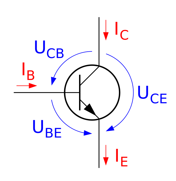

Some months back, I mentioned that I felt the sun-earth connection was much like a transistor. This new NCAR study suggests this may be the case where small solar variances are amplified in the earth atmosphere-ocean system.
From EurekAlert
Small fluctuations in solar activity, large influence on the climate
Sun spot frequency has an unexpectedly strong influence on cloud formation and precipitation
Our sun does not radiate evenly. The best known example of radiation fluctuations is the famous 11-year cycle of sun spots. Nobody denies its influence on the natural climate variability, but climate models have, to-date, not been able to satisfactorily reconstruct its impact on climate activity.
Researchers from the USA and from Germany have now, for the first time, successfully simulated, in detail, the complex interaction between solar radiation, atmosphere, and the ocean. As the scientific journal Science reports in its latest issue, Gerald Meehl of the US-National Center for Atmospheric Research (NCAR) and his team have been able to calculate how the extremely small variations in radiation brings about a comparatively significant change in the System “Atmosphere-Ocean”.
Katja Matthes of the GFZ German Research Centre for Geosciences, and co-author of the study, states: „Taking into consideration the complete radiation spectrum of the sun, the radiation intensity within one sun spot cycle varies by just 0.1 per cent. Complex interplay mechanisms in the stratosphere and the troposphere, however, create measurable changes in the water temperature of the Pacific and in precipitation”.
Top Down – Bottom up
In order for such reinforcement to take place many small wheels have to interdigitate. The initial process runs from the top downwards: increased solar radiation leads to more ozone and higher temperatures in the stratosphere. “The ultraviolet radiation share varies much more strongly than the other shares in the spectrum, i.e. by five to eight per cent, and that forms more ozone” explains Katja Matthes. As a result, especially the tropical stratosphere becomes warmer, which in turn leads to changed atmospheric circulation. Thus, the interrelated typical precipitation patterns in the tropics are also displaced.
The second process takes place in the opposite way: the higher solar activity leads to more evaporation in the cloud free areas. With the trade winds the increased amounts of moisture are transported to the equator, where they lead to stronger precipitation, lower water temperatures in the East Pacific and reduced cloud formation, which in turn allows for increased evaporation. Katja Matthes: “It is this positive back coupling that strengthens the process”. With this it is possible to explain the respective measurements and observations on the Earth’s surface.
Professor Reinhard Huettl, Chairman of the Scientific Executive Board of the GFZ (Helmholtz Association of German Research Centres) adds: “The study is important for comprehending the natural climatic variability, which – on different time scales – is significantly influenced by the sun. In order to better understand the anthropogenically induced climate change and to make more reliable future climate scenarios, it is very important to understand the underlying natural climatic variability. This investigation shows again that we still have substantial research needs to understand the climate system”. Together with the Alfred Wegener-Institute for Polar and Marine Research and the Senckenberg Research Institute and Natural History Museum the GFZ is, therefore, organising a conference “Climate in the System Earth” scheduled for 2./3. November 2009 in Berlin.
Berry R,
Thanks for the link (duplicated below) about California heatwaves, which documents a phenomena I have noticed here in Australia as the cause of very hot days and nights.
However, note the following quote,
Humidity is the key ingredient forming muggy nighttime heat waves. That same humidity usually provides some daytime relief by stoking afternoon cloud formation. The authors note that in the 2006 event, however, and to a lesser degree in the next largest 2003 event, the convection that usually triggers afternoon cooling was stifled.
You can’t ‘stifle’ convection. It’s a basic physical process. The cause of reduced cloud formation has to be reduced humidity in the column of air above the Earth;s surface, ie the humidity which caused the extreme heat must be in a thin band near the surface.
Changes in Pacific surface temperatures can’t produce the phenomena of a thin band of humidity near the surface in California and the cause is highly likely to be irrigation together with a lack of wind to distribute the humidity away from the surface.
I’ll be charitable and assume the authors merely got it wrong. Rather than conclude they deliberately avoided anthropogenic irrigation as the cause of the heat waves, as that would be too controversial (heretical?) a conclusion in the current political climate .
http://www.sciencedaily.com/releases/2009/08/090825151008.htm
Leif Svalgaard (15:21:34) :
“Thus is the standard nonsense. UV is 105 W/m2 vs. total TSI 1361 W/m2. 7% [mean of 5 and 8] of UV is 105*0.07=8 W/m2. TSI only varies 1.5 W/m2, and UV is but a small part of TSI.”
If your numbers are right that equation might work if we are considering the full UV spectrum. But it does not apply if we are looking at specific wave lengths which make up that spectrum.
From wikipedia about the 2006 California heatwave,
The most severe death toll was in California, principally in the interior region.[22] By the end of July, when the sweltering heat in California subsided, but the number of confirmed or suspected heat-related deaths climbed to 163 as county coroners worked through a backlog of cases.[1] A report from California Climate Change Center published in 2009 determined that the heat caused two to three times the number of deaths estimated by coroners in seven California counties. [23]
By July 25, California authorities documented at least 38 deaths related to the heat in 11 counties. Temperatures reached 110–115 °F (43–46 °C) in the central valley of California July 23–24.
So it seems the heat was concentrated in the agricultural areas and irrigation levels would have been particularly high to protect crops during the heatwave.
It would be interesting to see a more detailed breakdown of the extreme heat, but I doubt we will, because if I am right about irrigation as the cause, then it would undermine the AGW ‘consensus’.
Note, the period would have undoubtably have been very hot without the extra humidity from irrigation. However, irrigation would appear to be the additional factor causing the record temperatures.
Leif Svalgaard (15:21:34) :
“Thus is the standard nonsense. UV is 105 W/m2 vs. total TSI 1361 W/m2. 7% [mean of 5 and 8] of UV is 105*0.07=8 W/m2. TSI only varies 1.5 W/m2, and UV is but a small part of TSI.”
Do I understand that when UV increases, then some other portion of the total spectrum decreases? This is the only way I can see that UV varying by 8W/m^2 is consistent with TSI varying by only 1.5W/m^2.
Meteologically speaking, yes, via a cap or ‘capping inversion’ can inhibit convection. We have this condition quite often in Tejas (boundary layer quite warm and moist, but no convection). Perhaps this mechanism is not at play in this circumstance either?
Per Wikipedia on the subject: “A capping inversion limits the vertical development of clouds (convection)”
.
.
.
Thanks to my critics here I can now refine my propositions as follows:
1)The oceans behave similarly to an electrical resistor in that they receive solar shortwave energy, convert it to infra red longwave and generate a higher temperature in the process because that infra red longwave is then represented by greater vibration of the water molecules.
2)The oceans behave unlike an electrical resistor in that they can retain that energy within themselves by moving the energy around between oceanic molecules for very variable lengths of time before it is released to the air above.
3)That retention of energy is merely part of the one way flow of energy from sun to sea to air to space and so the energy cannot be ‘held’ in the conventional sense because a reduction in incoming energy will immediately alter the balance between incoming and outgoing energy and any surplus in the oceans will start to decline.
4) The oceans do not slow down the speed of electromagnetic energy but they do slow down the transmission of that energy through the Earth system by altering the rate at which it is released to the air.
5)The oceans behave like a capacitor in the way they can build up and release a ‘charge’ of heat energy to the air above.
6) The oceans behave unlike a capacitor in that instead of smoothing out the flow of power they instead introduce large discontinuities in the flow by intermittently accelerating and decelerating the flow of energy into the air.
7) It is the irregularity in the release of the flow of solar energy to the air that creates the apparently large discrepancy between the very small solar variability and the much larger energy budget changes observed in climate change.
8) The oceans do not ‘amplify’ solar variability in the usual sense because no increase in total energy can be effected. Instead, the oceans create their own discontinuities in the flow of solar energy through the Earth system and that involves both amplification and suppression of the solar signal rather than simple amplification.
9) Once the oceans introduce such discontinuities in the energy flow then the only way the Earth system can remain stable is for the air circulation systems to make opposing (negative) adjustments. It must be successful in doing so or we would have no oceans.
Suggestions for further refinement will be welcomed.
Jim Arndt (16:05:09) :
“This is the standard nonsense. UV is 105 W/m2 vs. total TSI 1361 W/m2. 7% [mean of 5 and 8] of UV is 105*0.07=8 W/m2. TSI only varies 1.5 W/m2, and UV is but a small part of TSI.”
The article said [try to actually read some of this stuff]: “”The ultraviolet radiation share varies much more strongly than the other shares in the spectrum, i.e. by five to eight per cent, and that forms more ozone” explains Katja Matthes.”
So, the researcher claims that UV varies 5-8% [call it 7%]. Of the 1361 W/m2 that is TSI, the part below 400 nm is called UV [the part below the UV band is inconsequential] and is 105 W/m2. For this to vary 7%, it must vary 105*7/100 = 8 W/m2, but the total [TSI] only varies by 1.5 W/m2.
Kevin Kilty (20:02:33) :
Do I understand that when UV increases, then some other portion of the total spectrum decreases?
Of course not. I was pointing out that the statement by the article that UV varies 5-8% is incorrect. The variation of UV can be no larger than (total variation of TSI = 1.5 W/m2)/(amount of UV=105 W/m2) = 1.5/105 = 1.5% and is actually less as some of the total variation is not in the UV.
maksimovich (17:08:02) :
The maximum sensitivity of the upper stratospheric temperature response is of about 0.16K per 1% change in solar radiation
What has that to do with anything?
I have a quetion for Dr Svalgaard.
Let us assume that the average magnitude of the heat energy transfer from the sun is more or less constant over the last centuries. Now if we further assume that although the exact physical mechanism is not yet known, the sun earth relationship can be viewed as a forced oscillator. Think of the analogy with pendulum or an electrical oscillatory circuit that is being externally driven. In a forced oscillator, it is important to know the resonance frequency of the system being driven but also the frequency of the external driving force. Now, let us assume that the earth’s eigenfrequency (if such a notion is at all meaningful) is somewhat shorter than 11 years. Then it will follow that the earth will tend to store more heat during shorter sun cycles as an oscillator oscillates better when is being driven closer to its resonance frequency. May this explain the Science paper by Friis-Christensen and Lassen (1991) where longer cycles tend to have a cooling effect? If this is the case, may we see a somewhat larger temperature decrease during the Eddy Minimum the next couple of years than previously expected from studying heat transfer from the sun only? (assuming that this is constant)
[Obviously the earth may have many different resonant or eigenfrequencies, but still the analogy above may be useful to cover the most predominant effects.]
[[Surely the forced oscillator is a toy model]]
“You can’t ’stifle’ convection. It’s a basic physical process. ”
In a lab maybe, but weather will set up temperature inversions with height (air temp. goes up with increasing height for a thousand feet or more), which indeed stifle convection and lead to cloudless heat-waves.
Invariant (01:31:36) :
the sun earth relationship can be viewed as a forced oscillator.
To have an oscillation, you must have a restoring force. What is the restoring force?
May this explain the Science paper by Friis-Christensen and Lassen (1991) where longer cycles tend to have a cooling effect?
The paper is bogus. Direct observation shows the opposite effect, if any [most likely there is none]. http://www.leif.org/research/Cycle%20Length%20Temperature%20Correlation.pdf
Thanks Dr. Svalgaard,
I am very unfamiler with climeate research but I am fairly skilled with analogies. (like in Feynman Lectures on Physics!) Thus I cannot easily suggest what may be the origin of a restoring force, but maybe someone with insight into climate cab help me? See the harmonic oscillator.
http://en.wikipedia.org/wiki/Harmonic_oscillator#Damped_harmonic_oscillator
I see that you are not fond of the 1991 Science paper, but could you try to explain, by using simple analogies, what is wrong with their approach?
Invariant (03:19:37) :
I see that you are not fond of the 1991 Science paper, but could you try to explain, by using simple analogies, what is wrong with their approach?
Let me explain my graph http://www.leif.org/research/Cycle%20Length%20Temperature%20Correlation.pdf
You van measure the length of a cycle in two ways: from min to min or from max to max. The blue curves show the cycle lengths measured the two ways [hence the two blue curves], with the cycle length plotted at the midpoint of each cycle. One can now calculate the average temperature for each cycle and plot the same way. this gives you the pink curves. The 2nd Figure shows the lack of correlation between the temperature and cycle length [pink circles]. One can try to remove the trend from the temperature curves. That gives you the green curves.
So, basically there is no correlation. Now, if you smooth the data enough you will always get a correlation. Image you compute the mean length and temperature for the first half of the data and for the last half. That gives you two data points, through which you can draw a line with correlation coefficient 1. If you don’t go this extreme, but smooth a bit less, you don’t get this perfect correlation, but still way more than for the raw [real] data. F&L smooth over 50 years. Since that would exclude the last 25 years, they change the smoothing [in the end don’t do any at all] for these years only, to be able to have ‘modern’ points. This is bad science. As I showed, the raw data don’t show any effect.
Leif Svalgaard (00:35:50) :
Kevin Kilty (20:02:33) :
Do I understand that when UV increases, then some other portion of the total spectrum decreases?
Of course not. I was pointing out that the statement by the article that UV varies 5-8% is incorrect. The variation of UV can be no larger than (total variation of TSI = 1.5 W/m2)/(amount of UV=105 W/m2) = 1.5/105 = 1.5% and is actually less as some of the total variation is not in the UV.
Leif is being less than honorable with his answer and is fully aware of what is really going on here. He is stating values related to the total UV content of the TSI value. UV is made of many components, some having more influence on the climate than others (much to be learned). The different components vary substantially and are not observed at the higher level (total UV).
One component of the UV value will be lost in the overall UV count due to the numerous components, but might be the key to the Sun/Earth link.
but weather will set up temperature inversions with height (air temp. goes up with increasing height for a thousand feet or more), which indeed stifle convection and lead to cloudless heat-waves.
A temperature inversion during a humidity induced heat wave would require the air to be even hotter at altitude.
I very much doubt this occurs.
Thank you for taking the time to explain all this, Dr. Svalgaard, I really appreciate it! As you know I have not studied the climate at all, but I think it is fascinating to follow the lively discussion we have today. Regarding the Friis-Christensen and Lassen (1991) paper I think we can roughly divide the different climate scientist into four separate “schools”, that is one can state,
1. a strong correlation,
2. a weak correlation,
3. no correlation, or
4. no evidence.
for a correlation between solar cycle length and temperature anomaly. Before your answer I think I was more in favour of alternative 2 or 4 than 3 which seems to be your point of view. Maybe there is a weak or maybe tiny correlation but that the data we have is insufficient to give a significant result?
A couple of years ago I studied natural convection in some detail and also read the paper by Lorenz (1963) about deterministic nonperiodic flow
http://www.cc.uoa.gr/~pji/nonlin/lorenz.pdf
Lorenz demonstrated that only tiny modifications of the initial conditions may alter the resulting periodic motion significantly. I know such sensitive phenomena can be used in an argument to prove or disprove anything, but let us assume that there actually is (although we do not have significant data to support this yet) a very weak correlation between the solar cycle length and temperature anomaly. Then, since the climate is sensitive (Lorenz, 1963) then this may be amplified (transistor analogy!) in cases where the cycle becomes very long. This is just a wild guess, and I will have to think about your point of view before I make ip my mind. Nonlinear phenomena are very complex!
Geoff Sharp (04:54:51) :
He is stating values related to the total UV content of the TSI value.
As was the article. There was no mention of any particular wavelength region, instead: ““The ultraviolet radiation share varies much more strongly than the other shares in the spectrum, i.e. by five to eight per cent, and that forms more ozone” explains Katja Matthes.”
There are wavelength regions [“shares” to use her word] that vary several hundred percent, but when you don’t specify the precise region the whole is clearly meant.
Invariant (06:02:04) :
Maybe there is a weak or maybe tiny correlation but that the data we have is insufficient to give a significant result?
If there is a correlation at all, it is opposite of what F&L claimed [and the main problem with their paper was the inappropriate analysis]. A negative result [‘no correlation’] can be highly significant. Anyway, if their is insufficient data, then the ‘finding’ should not be used at all.
Some of my replies below may be inconsequential. But some of your statements are just not valid! Sorry!
Stephen Wilde (00:27:51) :
1)The oceans behave similarly to an electrical resistor in that they receive solar shortwave energy, convert it to infra red longwave and generate a higher temperature in the process because that infra red longwave is then represented by greater vibration of the water molecules
The solar input is converted to heat. Heat generates long wave IR.
http://hyperphysics.phy-astr.gsu.edu/HBASE/wien.html#c3 (excellent stuff have a look)
20C is equivalent to 9885.72nm is equivalent to 30612.2449GHz
4C is equivalent to 10456.43nm is equivalent to 28690.47619GHz
2)The oceans behave unlike an electrical resistor in that they can retain that energy within themselves by moving the energy around between oceanic molecules for very variable lengths of time before it is released to the air above.
Conduction is fast. The oceans can retain heat by moving it away from somewhere where it can dissipate otherwise it is simply in balance with heat loss vs energy input. If 5deg C water is surrounded by 4degC water the two are continually try to equalise – in a static (is this possible?) situation there will be a continual transfer of energy across the 4/5C boundry creating a graduated 5C to 4C gradient. As time progresses this boundary will grow in width until all the water is at the average temp.
3) ok
4) ok (just about)
5)The oceans behave like a capacitor in the way they can build up and release a ‘charge’ of heat energy to the air above.
Capacitors store and release energy continually. If the voltage on the capacitor is less than the voltage feeding it (via an impedance) the capacitor will store energy. should the voltage feeding it fall below the capacitor terminal voltage the capacitor will discharge and loose energy. Your termonology seems to suggest a sudden release of energy to the air – this will not be the case.
If a capacitor is discharged then fluctuations in the charging voltage will not extract energy from the capacitor unless those fluctuations fall below the voltage to whic the capacitor is charged. All that will happen is that the energy flowing INTO the capacitor will rise and fall. With sea temperature if a hot day inputs energy to the sea and raises the surface layer to 20C then the next sun is occluded and the air temp falls below 20C the small amount of energy in the sea surface will momentarily keep the air warmer. Your single capacitor ocean will not work this way!
6) The oceans behave unlike a capacitor in that instead of smoothing out the flow of power they instead introduce large discontinuities in the flow by intermittently accelerating and decelerating the flow of energy into the air.
This is just simply incorrect the energy is always in balance at the surface. You still have not said how water heated from 4C to 5C at depth in the ocean is going to heat the air at 17C above.
7) It is the irregularity in the release of the flow of solar energy to the air that creates the apparently large discrepancy between the very small solar variability and the much larger energy budget changes observed in climate change.
see 6 response
8) The oceans do not ‘amplify’ solar variability in the usual sense because no increase in total energy can be effected. Instead, the oceans create their own discontinuities in the flow of solar energy through the Earth system and that involves both amplification and suppression of the solar signal rather than simple amplification.
How?????
9) Once the oceans introduce such discontinuities in the energy flow then the only way the Earth system can remain stable is for the air circulation systems to make opposing (negative) adjustments. It must be successful in doing so or we would have no oceans.
explain using scientific principles please.
Geoff Sharp (04:54:51)
I tried to get at that point a while back but the replies were unhelpful. Either I was failing to get the point across or there was ‘avoidance’.
We all know that total TSI varies very little.
Of the TSI a lot gets reflected in the air or obstructed before it gets to the ocean surface. Of the portion that gets to the ocean surface much is reflected by the ocean surface and another portion fails to get past the region involved in evaporation.
Only a tiny portion of TSI actually gets deeply enough into the ocean to make any difference to ocean energy content and some wavelengths are more successful than others.
If one identifies the tiny proportion of the limited number of specific wavelengths that are able to affect ocean energy content we must find that it is only a tiny part of TSI.
So, if the oceans do what they do with, say, only 1% of TSI then the value of TSI itself is irrelevant. 99% of it has no effect on ocean energy content.
Then if that 1% is subject to a greater level of variation than the variation seen in TSI the effect on the oceans will be greater than one would expect from the TSI variations.
Which wavelengths are most successful at getting below the evaporative layer and how much do they vary ?
Leif says that the variation in that 1% cannot exceed the variation in TSI.
That’s as maybe. I don’t think it needs to nor is it ever likely to. If the relevant 1% (or whatever) doubles or halves then that change is not going to make much dent on,say, 1.5% of TSI but it is going to double or halve the effect on the ocean energy budget. I’m not a mathematician so if that’s wrong I’m sure someone will say so and explain why for my benefit and that of passing readers.
I don’t propose that it does double or halve. Small changes could set a new temperature trend.
In fact all it needs to do is provide a long term global trend in the background which is what we actually see. The oceans themselves do all the rest.
During the time that UV has been measured by satellites there have been 2 peaks of TSI
If there was a significant increase in UV during TSI peaks then these would show up on the satellite data:
http://ozonewatch.gsfc.nasa.gov/
Thishas 2 little plots showing ozone peak during 1988 and 2002
However, 1988 does not correspond to a peak of tsi
tsi peaks (start of tsi decline) are 1992 and 2002
or looking at the peak flattening off from the rise 1989 an 2000
Bill (08:43:53)
Thanks for that. I can see how to make it clearer and more technically precise. The capacitor analogy was not mine. I was just seeing whether it could be worked in.
The point you miss is the real world observation of oceanic phase shifts at 25 to 30 year intervals.
There is a clear change in the rate of energy release by the oceans.
Here is the revised effort having abandoned the capacitor analogy:
Thanks to bill I can now further refine and simplify my proposition as follows:
1) The oceans behave similarly to an electrical resistor in that they receive solar shortwave energy, convert it to heat which generates infra red longwave and causes a higher temperature in the process because that infra red longwave is then represented by greater vibration of the water molecules.
2) The oceans behave unlike an electrical resistor in that they can retain that energy within themselves by moving the more energetic water molecules around within the oceans for very variable lengths of time before their energy is released to the air above.
3) That retention of energy is merely part of the one way flow of energy from sun to sea to air to space and so cannot be ‘held’ in the conventional sense because a reduction in incoming energy will immediately alter the balance between incoming and outgoing energy and any surplus in the oceans will start to decline.
4) The oceans do not slow down the speed of electromagnetic energy (except to a small degree while it is in the water) but they do significantly speed up and slow down the transmission of that energy through the Earth system by altering the rate at which it is released to the air. We have observed that in the multi decadal oscillations such as the phase shift seen in the Pacific every 25 to 30 years when the ocean surfaces switch from net warming to net cooling of the air above.
5) It is that irregularity in the release of the flow of solar energy to the air that creates the apparently large discrepancy between the very small solar variability and the apparently much larger energy budget changes observed in climate change. It is currently unclear why or how it happens.
6) The oceans thus create their own irregularities in the flow of solar energy through the Earth system and that involves both amplification and suppression of the solar signal. The size of the amplification or suppression is related to the characteristics of the oceans and that can change over time. The low level of solar variation can only ever provide a background trend.
7) Once the oceans introduce such discontinuities in the energy flow then the only way the Earth system can remain stable is for the air circulation systems to make opposing (negative) adjustments. It must be successful in doing so or we would have no oceans. I have described that process in general terms elsewhere but to be brief:
i) When the oceans release energy faster the air pushes energy to space faster thus limiting the warming of the air.
ii) When the oceans release energy more slowly the air tries to pull more energy
from the oceans thus trying to limit the cooling of the air.
Dear Dr. Svalgaard,
I can understand your concern about the Friis-Christensen and Lassen paper
(1991) – in particular since it is now cited 473 times according to Google Scholar. What the future may bring is not easy to tell, but surely the paper must be regarded as seminal in the discussion the last two decades. In my career as a scientist and engineer I have learned the hard way that one has to distinguish between what is possible to calculate and what is not possible to calculate. I have this beautiful quote from the Norwegian author Jens Bjørneboe that reveals this clearly,
”Man vet hvor en planet befinner seg om tolv år, fire måneder og ni dager. Men man vet ikke hvor en sommerfugl vil være fløyet hen om et minutt.”
— Jens Bjørneboe
This leads us to another butterfly-effect that is the famous and elegant metaphor introduced by Lorenz,
“When our results concerning the instability of nonperiodic flow are applied to the atmosphere, which is ostensibly nonperiodic, they indicate that prediction of the sufficiently distant future is impossible by any method, unless the present conditions are known exactly. In view of the inevitable inaccuracy and incompleteness of weather observations, precise very-long-range forecasting would seem to be non-existent.”
— Edward N. Lorenz
http://www.cc.uoa.gr/~pji/nonlin/lorenz.pdf
Most likely both the oscillations inside the sun and the oscillations in our climate are dominated by unpredictable buoyancy forces of the same nature as described in the famous Lorenz paper. Then what chance do we have to predict the climate? My initial analogy with a forced oscillator may not be so helpful either. In particular as most intrinsic oscillations in the sun and the oceans are obviously highly nonlinear. In software we can simulate such nonlinear oscillators with high precision. For example we can learn that tiny a butterfly can prolong the period of a relaxation oscillation indefinitely, just like the “transistor effect” proposed in the latest issue of Science by Meehl et al.
http://www.sciencemag.org/cgi/content/abstract/325/5944/1114
But this cannot be used to predict anything; it is time yet again to mention that climate simulations lag so far behind experimental evidence that no one would blame you for believing that the two main sets of people that determine your climate future are living on two planets in separate solar systems light years away.
“True knowledge is when one knows the limitations of one’s knowledge.“
If one draws a sphere around the earth and its atmosphere , Stefan-Boltzmann/Kirchhoff specifies the mean temperature over that sphere as a function of the millionth of the sky subtended by the sun at around 6000k and the all the rest at near 0 . It works out that objects in our orbit are constrained to be about 1%21 the temperature of the sun . It is a mistaken notion that average absorptivity/emissivity ( gray value ) will affect that ratio . I have this basic function now implemented in several Array Programming Languages on my http://CoSy.com and would love to see someone translate it into more common languages like Mathematica or MatLab . It currently handles any angular distribution of gray value , eg , differences between day and night sides , or latitude . I am extending the function to full spectra so that the extreme any lumped spectral distribution ( 1.0 correlated with the sun ) could produce , or the calculated effect of some delta in CO2 saturation .
( The above would be rejected as gibberish on a realityDenier blog ; their talent sure ain’t basic physics . )
A couple of major points :
Lumped earth/atmosphere temperature is linear with sun temperature . Any nonlinearities within this envelope must cancel by this boundary . Any discussion of “runaways” and “feedbacks” macht nichts . The SB/K equation has held up to at most a few percent of earth/sun temperature ratio . The idea that we are at some particular ratio where some nonlinearity occurs is non-sensical .
It’s useful to keep in mind that the total change in temperature we’ve seen a century is only about 1%300 = 0.33% . I’m delighted that the sun is that constant .
Stephen Wilde (08:44:34) :
Leif says that the variation in that 1% cannot exceed the variation in TSI.
The fundamental error that people commit is to express variation as a percentage. What matters is the variation of the actual amount of energy involved. For TSI that is 1.5 W/m2. For UV the variation is about 0.3 W/m2, for the very energetic part less than 0.03 W/m2. While the relative variation in % gets larger as we go towards shorter wavelengths, the actual energy we get gets smaller and smaller, so it matters not much what the variation is. It is like basing the credit worthiness of someone by the variation of loose change in his pocket rather than the value of his house.
Invariant (11:57:00) :
I can understand your concern about the Friis-Christensen and Lassen paper (1991) – in particular since it is now cited 473 times according to Google Scholar. What the future may bring is not easy to tell, but surely the paper must be regarded as seminal in the discussion the last two decades.
It will be held up as a warning of how easily people will go along with bad science as long as it supports their views. Perhaps AGW is another example. And this without even reading the paper. In the F&L paper they say [from memory] that “solar activity might influence climate, and since it is well-known that the size of a cycle depends on its length [not always so, actually], then we can use the length as a proxy for the size”. Then they go on working with the length [heavily smoothed to boot]. Good science would not use a proxy for something if that something is directly available.