A Holocene Temperature Reconstruction Part 1: the Antarctic

By Andy May

The only recent attempt at a global Holocene temperature reconstruction available today is the one by Marcott, et al. (2013), the paper abstract can be viewed here. His reconstruction is shown in figure 1.

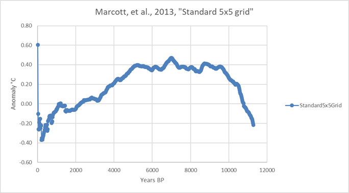
Figure 1

The Y axis is a reconstructed global temperature anomaly from the 1961-1990 mean. “Years BP” are years before 1950. This reconstruction shows a fairly flat Holocene Climatic Optimum (or HCO, also called the Holocene Thermal Optimum, see description here) temperature anomaly of +0.4°C from 9500 BP to 5000 BP, declining to a low of -0.4°C about 300 BP (1650 AD) in the Little Ice Age (LIA). This 0.8°C difference between the HCO and the LIA is smaller than the generally accepted difference of 1°C to 1.5°C. This is documented in some detail by Javier here. The higher accepted difference is clear in glacial records as shown by Koch, et al., 2014 (link). It can also be seen in the biosphere as shown by Kullman 2001 (link); Pisaric et al. 2003 (link); MacDonald et al. 2000 (link); Tinner, et al. 1996 (link) and Thouret et al. 1996 (link)). Further, the marine biosphere also shows a larger temperature difference as seen in Werne et al., 2000 (link) and Rosenthal et al., 2013 (link).

The reconstruction in figure 1 goes from the present (1950) on the left to nearly the beginning of the Holocene about 11,700 years ago on the right. The Holocene is normally defined as “the first signs of climatic warming at the end of the Younger Dryas/Greenland Stadial 1 cold phase” (Walker et al. 2009). It is often considered a geological epoch or series. It is part of the Quaternary geological period and is equivalent to the older geological term “Recent.”

The reconstruction shows an abrupt warming in the last 100 years (see the left side of figure 1). This single point at 1940 AD is due to proxy drop out, proxy inconsistencies and the authors changing some published dates in the proxies according to Steve McIntyre at climateaudit.org here, here and here. Also see “The Tick” by Grant Foster here for more discussion, the first comment to “The Tick” is by our own Nick Stokes. Even Marcott has acknowledged that his reconstruction from 1890 AD onward is not robust. The following quote is by Marcott, here.

“We showed that no temperature variability is preserved in our reconstruction at cycles shorter than 300 years, 50% is preserved at 1000-year time scales, and nearly all is preserved at 2000-year periods and longer. Our Monte-Carlo analysis accounts for these sources of uncertainty to yield a robust (albeit smoothed) global record. Any small “upticks” or “downticks” in temperature that last less than several hundred years in our compilation of paleoclimate data are probably not robust, as stated in the paper.”

The problem is that 300 years is a very long time. As we will see, many very significant climatic events begin and end in less than 300 years. Marcott et al. (2013) chose too many proxies with poor temporal resolution, which reduced the resolution of their reconstruction to the point that significant details were lost.

This is a new look at Marcott’s proxies. It is a good collection and most of them are marine sea surface temperature proxies. This is a good thing because most of the heat energy or heat capacity on the Earth’s surface is in the oceans. In fact, over 99.9% of the surface heat content is in the oceans and only 0.071% is in the atmosphere, for the details of this calculation see the spreadsheet here. Warming of the atmosphere is not particularly significant on a climatic scale.

It is very logical to investigate long term climate changes using ocean temperature proxies from foraminifera shells and fossils (“forams”), planktonic and algal material. Traditionally the magnesium and calcite (Mg/Ca) percentages or d¹⁸O ratios in planktonic foraminifera have been used to deduce ancient sea surface temperatures. On land, ice core d¹⁸O records and pollen are used to estimate ancient air temperatures. More recently we have seen more use of haptophyte algal alkenones, especially the U₃₇^K’ (also written as UK’37) index to get ancient sea surface temperatures, see the link here. TEX₈₆ records from marine plankton have also been used recently to obtain sea surface temperatures and are among Marcott’s proxies, see here for a discussion. The original reference for the TEX₈₆ sea surface temperature proxy is Schouten, et al. (2002) here. A complete list of the proxies used by Marcott, plus one I added from Rosenthal, et al. (2013) and references and links to the original papers can be downloaded here. I did not use all Marcott’s proxies in my reconstructions, those that I did use are noted in the spreadsheet.

Proxy selection

The proxies were examined considering the criticism of Marcott’s analysis by Javier, McIntyre and Foster. The 500-meter depth Indonesian ocean proxy presented in Rosenthal, et al. 2013 was added to the list. Proxies used in this reconstruction were selected using the following criteria:

1. The span of the proxy reconstruction had to cover at least 600 BP to 8000 BP so the proxy covered part of the LIA and the HCO.
2. The resolution (time between samples) had to be less than 130 years.
3. Complex statistical techniques were avoided as much as possible.

The major climatic events of the Holocene are the Holocene Climatic Optimum (HCO) and the Little Ice Age (LIA), these events represent the maximum global average temperature and the minimum temperature respectively in this period. As noted above, there is abundant evidence that the global temperature difference between these two points exceeds one degree Celsius. Therefore, it seems logical to make sure the proxies cover both events. Further, since all the reconstructions are temperature anomalies, we have built the anomalies as differences from the proxy mean between 9000 BP and 500 BP.

There is concern that the reason the Marcott, et al. (2013) reconstruction is underestimating the LIA to HCO temperature difference is that they included too many proxies with very long sample intervals. Proxies with long sample intervals miss essential detail and smooth and dampen detail in any reconstruction. Just averaging too many proxies can dampened detail if there is error in the proxy dates.

Climate changes over the Holocene occur, in large part, by latitude. This is due to the Earth’s orbital obliquity (amount of axial tilt which changes over a 41,000-year cycle) and precession (wobbling of the axis over 19,000 to 23,000 years) cycles, as well as the long-term transport of heat by ocean currents. This is explained well by Javier here. In the same post, Javier explains the orbital effects in this way:

“Changes due to obliquity have the effect of redistributing insolation between different latitudes following an obliquity cycle of 41,000 years. When obliquity was maximal 9,500 years ago, both poles received more insolation due to obliquity, while the tropics received less. Obliquity also affects seasonality, at maximal axial tilt, there is an increased difference between summer and winter at high latitudes. But unlike precession changes, obliquity alters the amount of annual insolation at different latitudes in a 41,000-year cycle. This is represented by the background color of figure 34, that shows how the polar regions received increasing insolation from 30,000 yr BP to 9,500 yr BP. Since then, and for the next 11,500 years, the poles will be receiving decreasing insolation. Unlike precessional insolation changes, obliquity changes are symmetrical. Although the annual insolation change is not too large, it accumulates over tens of thousands of years and the total change is staggering, creating a huge insolation deficit or surplus. This changes the equator-to-pole temperature gradient, and is largely responsible for entering and exiting glacial periods (Tzedakis et al., 2017) and for the general evolution of global temperatures and climate during the Holocene.”

The emphasis is in the original post. Javier’s figure 34 is presented below as our figure 2.

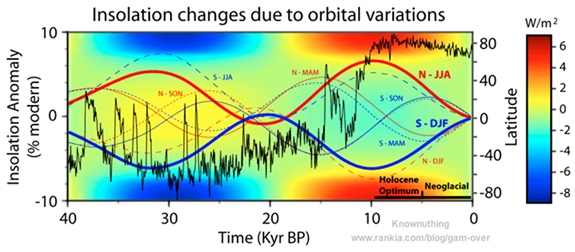
Figure 2

Javier’s description of this figure, in part:

“Figure 34 [our figure 2]. Insolation changes due to orbital variations of the Earth. The insolation changes for the last 40,000 years are represented. Black temperature proxy curve represents d¹⁸O isotope changes from NGRIP Greenland ice core (without scale). The insolation curves are presented as the insolation anomaly for summer, winter, spring, and fall. N (red) or S (blue) are the Northern or Southern Hemisphere and the three letters are the month initials. Northern and southern summer insolation represented with thick curves. Background color represents changes in annual insolation by latitude and time due to changes in the Earth’s axial tilt (obliquity), shown in a colored scale. … changes in obliquity … are symmetrical for both poles. Changes … caused by the precession cycle (modified by eccentricity) are asymmetric and less important for the global response, although they cause profound changes in regional climatic differences. The Holocene Climatic Optimum corresponds to high insolation surplus in polar latitudes (red area), while Neoglacial conditions represent the first 5,000 years of a 10,000 year drop into a high glacial insolation deficit in polar latitudes (blue area).”

Since latitude has such a large influence on climate and climate changes, we will produce reconstructions in 30° regions of latitude. The Antarctic region, with latitudes from 90°S to 60°S is presented first in this post. In the next post, we will present reconstructions for the southern hemisphere mid-latitudes (60°S to 30°S) and for the tropics (30°S to 30°N). The northern hemisphere mid-latitudes and the Arctic will follow in part 3. Our final global reconstruction will be a combination of these. It is presented in part 4.

The Marcott, et al. (2013) reconstruction is based upon 5° by 5° global grid created using their proxies. Gridding data is an accepted way of spreading unevenly spaced data evenly over a map, but it can cause distortions. The distortions can occur due to isolated, but extreme values or because the values gridded are incompatible, or simply because of data clustering, that is many values in one part of the map, see an example here. Table 1 shows the distribution of the proxies used in this series.

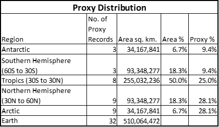
Table 1

The Marcott, et al. (2013) proxies are much more numerous in the northern hemisphere than in the south, so for this reason, we chose not to grid the data, but instead create five simple latitude bounded regional reconstructions and merge them. A great effort was made to make the process used as simple as possible and completely reproducible. All calculations were done with R, a statistical software package that is available for free (see here). As you can see in table 1, only 19% of the proxies that meet our criteria fall in the southern hemisphere below 30°S, which is 25% of the Earth. The same 25% area in the northern hemisphere contains 56% of the proxies. We hope that using our method will reduce any distortion introduced by the proxy distribution.

All R code and the R input and output text files will be made available in the supplementary materials for each post. We also provide spreadsheets containing metadata, references and plots of the original proxy temperatures. No error analysis has been done on these reconstructions, but this should be done. Readers are encouraged to use my code and data to do their own error analysis. Ideas on how to separate the various error components, such as dating error, proxy error, geographic error, depth or altitude error, etc. are welcomed. One thing that complicates the computation of error, is that in some cases different proxies were used for the same core (see 74KL, in the Arabian Sea, by Huguet et al., 2006) and the resulting reconstructions were different. This could be due to seasonal differences, depth or altitude differences or due to local weather variability (Huguet, et al. 2006). In all cases I used the original published dates, no adjustments have been made except to align them to a 1950 reference which is the standard reference for “BP.”

The Antarctic reconstruction

The final Antarctic reconstruction is shown in figure 3. The curve is the anomaly from the 9000BP to 500 BP mean.

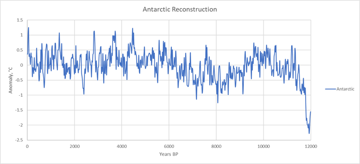
Figure 3

In the Antarctic reconstruction, we appear to see a slight Little Ice Age drop at 1230 AD. There are several peaks in the Medieval Warm Period from 1110 AD to 890 AD, but nothing very dramatic.

Marcott, et al. (2013) had four temperature proxies below 60°S. We selected three from this set, Vostok, Dome C and EDML. The proxy details and metadata are in the supplementary spreadsheet “Reconstruction_References.xlsx” which can be downloaded here. Dome F was rejected due to a 500-year resolution. These are all ice core proxies that estimate air temperature. A map of the proxies (see figure 4) shows that all are in East Antarctica.

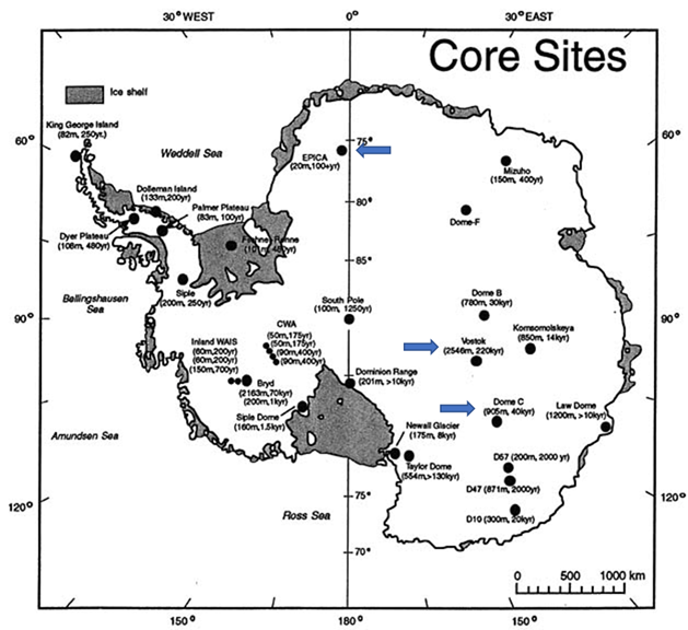
Figure 4

Figure 5 shows the three proxies used in the reconstruction. All of the proxies are anomalies from the 500BP to 9000 BP mean.

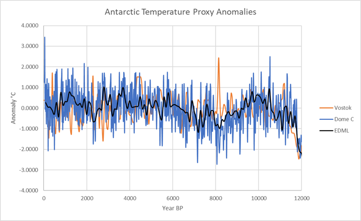
Figure 5

The three proxies generally agree with one another and the reconstruction, with minor suspicious looking differences such as the spike in the Vostok record at 8200 BP.

After reading the proxies into R, a matrix of reconstructed temperatures was created with a regular spacing of 20 years from -60 BP (2010) to 11980 BP (10,030 BC). This matrix is then populated with the proxies, taking care to average multiple values if they are within 11 years of the matrix date. Gaps in each proxy are filled with a cubic spline function allowing a maximum gap of 11 samples or 220 years. No extrapolation at the ends of the vectors was allowed, this is to reduce the chance of spurious spikes at the end of the proxy records.

After filling gaps table 2 shows the beginning of the matrix:

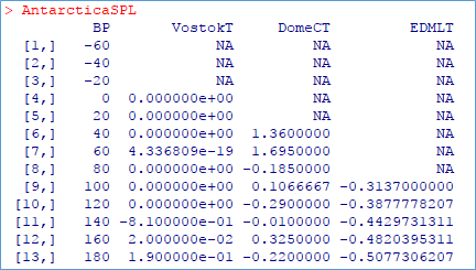
Table 2

Most of Marcott’s proxies contain actual estimated temperatures, but these proxies are all anomalies. The R missing value code is “NA.” The anomalies are from different means. The zeros from 0 BP to 120 BP in the Vostok column look suspicious, but they are in the Pettit, et al. (1997) data. By 100 BP (1850 AD) we have data for all three cores. Dome C shows warming from 100 BP to 40 BP, so the uptick at the end of the reconstruction is due to two points in one core. Table 3 shows the end of the matrix.

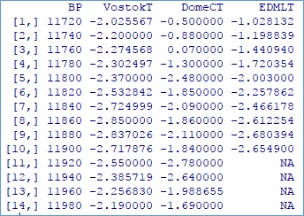
Table 3

All three cores show rapid warming from 11900 BP to 11720 BP. Each of the three proxies are converted to new anomalies from their individual mean temperatures from 9000BP to 500 BP, this is to give them all the same chronological basis. Finally, the Antarctic region reconstruction is created by averaging the three anomalies. The result is figure 3. Figure 6 is the same reconstruction, but plotted by R with an overlain smoothed curve.

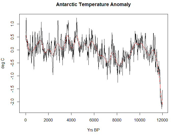
Figure 6

The graph shows Holocene climatic optima from 11000 BP to 9500 BP and 6000 BP to 3000 BP. The later period is slightly warmer than the earlier period which is very different from what is seen in the northern hemisphere and the other regions in this study. This result is similar to what has been reported by Masson, et al., 2000. Masson, et al. (2000) write:

“All the records confirm the widespread Antarctic early Holocene optimum between 11,500 and 9000 yr; in the Ross Sea sector, a secondary optimum is identified between 7000 and 5000 yr, whereas all eastern Antarctic sites show a late optimum between 6000 and 3000 yr.”

Unlike Masson, et al. (2000) we show the later optimum to be slightly warmer than the earlier one. But, the difference is only a few tenths of a degree and probably not significant. The choice of proxies can be critical when dealing with small differences in temperature. It is interesting to look at the variety of deuterium profiles presented by Masson, et al. (2000) in their figure 3, which is not reproduced here.

Likewise, the rapid warming out of the Younger Dryas seen in the northern hemisphere around 11500 BP appears to occur hundreds of years earlier in the Antarctic. It is also possible that there is no discernable Younger Dryas cooling in the southern hemisphere (Barrows, et al., 2007). Southern Ocean sea surface temperature reconstructions shown in Bostock, et al. (2013) (see their figure 3B, reproduced as our figure 7) show that the early temperature optimum in the Southern Ocean is quite variable. In some areas, it is at about 10000 BP and in others it is about 6000 BP. But, often the difference between the peaks is quite small and perhaps below the accuracy of the data.

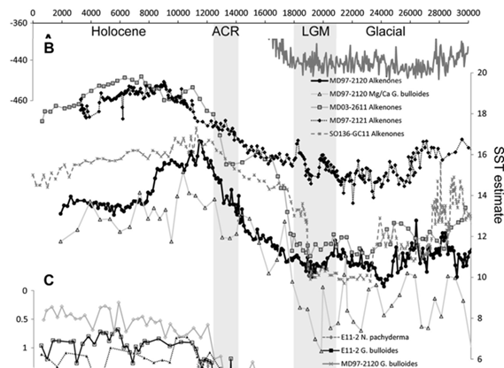
Figure 7 (source Bostock et al., 2013)

Our proxies are all eastern Antarctic land air temperature proxies and they reach a much later peak, around 6000 BP to 3000 BP by a few tenths of a degree.

Conclusions

The Marcott, et al. 2013 worldwide reconstruction has its problems, but many of the proxies used in the reconstruction are quite good and very usable.

The Antarctic reconstruction created here is comparable to previous temperature reconstructions, especially those focusing on eastern Antarctica. It shows two climatic optima, one from 11500 BP to 9000 BP and another from 6000 BP to 3000 BP. In eastern Antarctica, using our proxies, the later optimum is warmer. But, in other areas the earlier optimum is warmer, however, the difference is small.

In following posts, I will create similar reconstructions for the Arctic, the southern and northern mid-latitudes and one for the tropics. These will be area weighted and merged into one proposed global reconstruction in the final post.

The R code used to create this reconstruction and the input and output datasets can be downloaded here. The list of proxies used for all six reconstructions, the original references and links can be downloaded here.

I am very grateful to Javier who has read this post and made many very helpful suggestions. Any errors are the author’s alone.