From Dr. Roy Spencer’s Global Warming Blog
by Roy W. Spencer, Ph. D.
The Version 6 global average lower tropospheric temperature (LT) anomaly for August, 2024 was +0.88 deg. C departure from the 1991-2020 mean, up slightly from the July, 2024 anomaly of +0.85 deg. C.

Persistent global-averaged warmth was (unusually) contributed to this month by the Southern Hemisphere. Of the 27 regions we routinely monitor, 5 of them set record-warm (or near-record) high monthly temperature anomalies in August, all due to contributions from the Southern Hemisphere:
Global land: +1.35 deg. C
Southern Hemisphere land: +1.87 deg. C
Southern Hemisphere extratropical land: +2.23 deg. C
Antarctica: +3.31 deg. C (2nd place, previous record was +3.37 deg. C, Aug. 1996)
Australia: +1.80 deg. C.
The linear warming trend since January, 1979 now stands at +0.16 C/decade (+0.14 C/decade over the global-averaged oceans, and +0.21 C/decade over global-averaged land).
The following table lists various regional LT departures from the 30-year (1991-2020) average for the last 20 months (record highs are in red):
| YEAR | MO | GLOBE | NHEM. | SHEM. | TROPIC | USA48 | ARCTIC | AUST |
| 2023 | Jan | -0.04 | +0.05 | -0.13 | -0.38 | +0.12 | -0.12 | -0.50 |
| 2023 | Feb | +0.09 | +0.17 | +0.00 | -0.10 | +0.68 | -0.24 | -0.11 |
| 2023 | Mar | +0.20 | +0.24 | +0.17 | -0.13 | -1.43 | +0.17 | +0.40 |
| 2023 | Apr | +0.18 | +0.11 | +0.26 | -0.03 | -0.37 | +0.53 | +0.21 |
| 2023 | May | +0.37 | +0.30 | +0.44 | +0.40 | +0.57 | +0.66 | -0.09 |
| 2023 | June | +0.38 | +0.47 | +0.29 | +0.55 | -0.35 | +0.45 | +0.07 |
| 2023 | July | +0.64 | +0.73 | +0.56 | +0.88 | +0.53 | +0.91 | +1.44 |
| 2023 | Aug | +0.70 | +0.88 | +0.51 | +0.86 | +0.94 | +1.54 | +1.25 |
| 2023 | Sep | +0.90 | +0.94 | +0.86 | +0.93 | +0.40 | +1.13 | +1.17 |
| 2023 | Oct | +0.93 | +1.02 | +0.83 | +1.00 | +0.99 | +0.92 | +0.63 |
| 2023 | Nov | +0.91 | +1.01 | +0.82 | +1.03 | +0.65 | +1.16 | +0.42 |
| 2023 | Dec | +0.83 | +0.93 | +0.73 | +1.08 | +1.26 | +0.26 | +0.85 |
| 2024 | Jan | +0.86 | +1.06 | +0.66 | +1.27 | -0.05 | +0.40 | +1.18 |
| 2024 | Feb | +0.93 | +1.03 | +0.83 | +1.24 | +1.36 | +0.88 | +1.07 |
| 2024 | Mar | +0.95 | +1.02 | +0.88 | +1.35 | +0.23 | +1.10 | +1.29 |
| 2024 | Apr | +1.05 | +1.25 | +0.85 | +1.26 | +1.02 | +0.98 | +0.48 |
| 2024 | May | +0.90 | +0.98 | +0.83 | +1.31 | +0.38 | +0.38 | +0.45 |
| 2024 | June | +0.80 | +0.96 | +0.64 | +0.93 | +1.65 | +0.79 | +0.87 |
| 2024 | July | +0.85 | +1.02 | +0.68 | +1.06 | +0.77 | +0.67 | +0.01 |
| 2024 | August | +0.88 | +0.96 | +0.81 | +0.88 | +0.69 | +0.94 | +1.80 |
The full UAH Global Temperature Report, along with the LT global gridpoint anomaly image for August, 2024, and a more detailed analysis by John Christy, should be available within the next several days here.
Lower Troposphere:
http://vortex.nsstc.uah.edu/data/msu/v6.0/tlt/uahncdc_lt_6.0.txt
Mid-Troposphere:
http://vortex.nsstc.uah.edu/data/msu/v6.0/tmt/uahncdc_mt_6.0.txt
Tropopause:
http://vortex.nsstc.uah.edu/data/msu/v6.0/ttp/uahncdc_tp_6.0.txt
Lower Stratosphere:
http://vortex.nsstc.uah.edu/data/msu/v6.0/tls/uahncdc_ls_6.0.txt
Is this Southern contribution related to ENSO?
If it is then it is a very unusual ENSO compared to previous events in the record.
This entire post-El Nino peak is atypical. If the Hunga Tonga eruption isn’t responsible for this anomalous peak, then the experts need to be looking for another explanation.
El Niño and La Niña are two opposing climate patterns that break these normal conditions. Scientists call these phenomena the El Niño-Southern Oscillation (ENSO) cycle. El Niño and La Niña can both have global impacts
Thanks for once again showing us that you can’t comprehend a simple question.
The global impact of major El Ninos is totally obvious.. a spike and a step change.
So… Show us the global impact of La Ninas in the UAH data.
Or FAIL again.
So you FAILED again.. as expected.
The WUWT ENSO meter, found on the lower part of the right-hand column of this webpage below the listing of Bookmarks is currently reading 0.0 . . . smack in the middle of the “neutral” zone.
Hint to WUWT editors: it may be time to add another meter adjacent to the current one . . . call it the ENSO “delay time” meter, with a scale ranging from 0 to 24 months.
/sarc
I don’t get the /sarc tag?
Elevated UAH temperatures always persist for some lag period after the end of an El Nino event.
Please define “some lag period”, assuming it’s not two years or longer.
Hint: the /sarc tag is to reflect that there are no deterministic time lags or occurrence frequencies associated with ENSO events.
Enso meter is based on a small section of ocean in the middle f the ENSO region.
It does not show how wide-spread the El Nino effect is.
Are you sure about that?
WUWT editor Ric Werme maintains the WUWT ENSO meter and states that he obtains the relevant sea-surface temperature measurements from the Australian Bureau of Meteorology (BoM) . . . reference https://wattsupwiththat.com/2024/08/30/friday-funny-troll-or-serious/#comment-3962120
In turn, here is what the BoM itself has to say about calculating the ENSO:
“The Southern Oscillation Index, or SOI, gives an indication of the development and intensity of El Niño or La Niña in the Pacific Ocean. The SOI is calculated using the pressure differences between Tahiti and Darwin.”
(http://www.bom.gov.au/climate/about/?bookmark=enso )
FYI, the span distance between Tahiti and Darwin is 8,515 km . . . something few knowledgeable persons would classify as “small”.
No, probably not, just not letting it dissipate as it usually does.
Looks like some sort of stratosphere event causing the warming weather around Australia and the SH.
Record 50C temperature increase over Antarctica to shift Australia’s weather patterns – ABC News
The red text headline is, at best, an alarming half-truth for the associated hyperlinked ABC News article.
If you read the details in that article, you find the 50 °C increase is associated with a localized hot spot in the stratosphere off the east coast of Antarctica. It is not over the continent of Antarctica.
Furthermore, the article states the following:
“Technically the warming of the stratosphere is required to average at least 25C to be classified as a true SSW {sudden stratospheric warming}, and while this event’s warming has doubled that figure near the east Antarctic coast, the average warming over the whole of Antarctica may have so far peaked just below the threshold.”
with the graphic that I’ve posted here taken directly from under that statement in the article.
Two things to note:
1) the warming event took place at the 10 hPa level in the stratosphere and near the worst of the Antarctic winter,
2) the average warming over Antarctica at 10 hPa altitude at that time was only about one-third the average warming that occurs naturally between winter and summer over Antarctica.
Hmmmm . . . the “news” doesn’t appear to be really all that alarming when you look into the matter, as opposed to just reading the headline.
Unusual for this time of year, and what caused the latter half of August to be decidedly warmer than usual.
…
Guess what, the last couple of weeks of August were sort of unusually warm for this time of year.
Oh dear . . . there it is again, a dire warning of the POSSIBILITY of totally-undefined “extreme weather”.
Me? . . . I give that phrase all the importance that it deserves.
Definitely not, it is the water vapor from the HT eruption.
And it does not appear to be going away anytime soon in the Southern Hemisphere, the Northern Hemisphere is still under the effects but there are other factors at play.
Graphics produced by IDL (nasa.gov)
“it is the water vapor from the HT eruption.”
requires repeating. !!
The unusual warming over the last two years globally, seems like a slam dunk for HT. But I think there are a number of researchers out there that love WaveTran / ModTran more than they like anecdotal evidence.
The reason that Australia did not see records last year was because of the Brushfire particulates in the Stratosphere, in which the biggest fires were from 2019 – March of 2020. You can see on the middle plot of Australia UAH LT that temps were down considerably from 2021 until mid 2023. The particulates are gone now, and Australia is getting more sunlight. These are July values; it will be mid-month before August data is downloadable. The Stratosphere over Australia has been quite busy since 2016.
The top graph in your attachment defines the “lower stratosphere” over Australia to be at altitudes of 14–20 km.
I believe what you are discussing is more properly describing perturbations (including expansion in overall thickness/height) of the tropopause and not the stratosphere, which is never properly defined by reference to absolute altitude.
The Tropopause is available in the UAH catalog, the Lower Stratosphere and the Tropopause are disseminated by the UAH processing techniques.
The altitude range of all layers of the atmosphere vary with latitude, with the equator being the thickest portion and the poles being the thinnest. Those altitude ranges annotated in the title of the plot are global ranges, and not specific to Australia.
I did not provide the titles for each of the three graphs in the image that you provided above.
Assuming that you yourself did not create and title those graphs, I strongly suggest that you inform the source of those graphs (which I seriously doubt to be UAH) of your stated observations/corrections.
It is not my problem that you do not know what you are talking about. From prior experience with your comments and with your blatant lack of knowledge on the subject of atmospheric physics, I will thereby allow you to vent your chaos.
There can be no more contact, fire away.
Thank you for your permission.
“And it does not appear to be going away anytime soon in the Southern Hemisphere . . .”
It may, even, last forever!
Don’t be stupid. you make yourself look like fungal or RG
It is just dissipating rather slowly, as was initially predicted.
So, given your statements, what have you or others determined to be the exponential (or is it linear?) decay constant associated with the “dissipation”?
Remember, “don’t be stupid”.
So, you are determined to be stupid..
except maybe you don’t have a choice !
I think the upper troposphere changes are more important at the moment. This shows the water vapor is now reaching that altitude.
The Tropopause will be influenced by the radiative properties of the mid and upper stratosphere. Essentially it is feedback, because all IR leaving the planet must go through the Stratosphere, including the IR emanating from the cloud tops. One of the big problems here is there is very little known about the coupling of the radiative properties of the Stratosphere in conjunction with the Tropopause / Troposphere.
Research of these things are in their infancy at this moment in time, but this experiment by nature hopefully will shed light on how Earths energy budget really works. The claim made by many including the UAH team that significantly increasing water vapor in the Stratosphere will have little effect on the temperature of this planet appears to be based on invalid assumptions / physics.
Correct me of I’m wrong(I’m still learning the intricacies of the Globul Whaaming scam) but showing that HT is responsible for any of the alleged warming would be very inconvenient for the AGW cult. Because it takes away from their main theological point: that humans cause it.
So in no way are they inclined to point to any other possible information.
Climate scientists already accept that volcanoes can cause temperature changes. Afterall, it was climate scientists who discovered this. They even hypothesize that the HT eruption itself is partly the cause of the warming over the last couple of years and expect regional effects to last another 5 years.
HT being a contributing factor to warming is more inconvenient for contrarians because it would show that a mere 150 MtH2O was all it took. To put that into perspective 150 MtH2O represents only a 0.0003 ppm increase in the atmosphere.
Avoiding the main question, as usual.
What is the ppm in the stratosphere and not the whole atmosphere.
No, Australia’s sudden temperature rise is easily explained with a series of links from a very ‘progressive’ media outlet
“Not climate change but ‘natural phenomenon’
In September 2019 Australia’s ABC news reported on sudden stratospheric warming in Antarctica that lead to a spring spell of warming – that lasted months.
https://www.abc.net.au/news/2019-09-06/rare-weather-event-over-antarctica-drives-hot-outlook/11481498
.
In late July 2024 Australia’s ABC news reported that there was another outbreak of SSW – in which they reported that this would likely cause warming over Australia – that could last months
https://www.abc.net.au/news/2024-07-27/nsw-antarctica-warming-over-50c/104142332
.
On August 26th & 29th Australia’s ABC news reported that “Climate Change” was wholly responsible for the current August warm spell in Australia.”
https://www.abc.net.au/news/2024-08-26/winter-weather-40-degrees-in-august/104271368
https://www.abc.net.au/news/2024-08-29/winter-ends-with-heatwave-as-climate-change-upends-seasons/104279250
It is interesting how the temperature anomaly spiked up then plateaued, something not seen in previously in the record.
If you believe the UAH numerical data given in the table in the above article has a meaningful precision to the nearest 0.01 °C, then there hasn’t been any recent plateau in GLAT.
UAH claims an uncertainty of ±0.20 C for the monthly anomalies.
[Christy et al. 2003]
BFD. They don’t understand measurement uncertainty analysis any better than you (don’t).
So, why did you claim there is an acceleration of 0.028C per decade?
First…it is 0.0028 C per decade squared. Anyway that is what Excel’s LINEST function reports.
It is totally MEANINGLESS because it relies on one major El Nino event at the end of the record.
It is just a moronically stupid calculation to even bother doing with the data at hand.
Excel isn’t ‘smart’ enough to pick the correct number of significant figures. That is left up to you. Guess what?
Are you sure about that?
You tell me Clyde. Go ahead…tell me what the correct number of digits is? Don’t forget to show your work because you know I’m chomping at the bit to show you exactly what the standard error of the quadratic polynomial coefficient is and why I choose 2 significant figures. So yeah, let’s go down this rabbit hole shall we.
The last decimal place should match the uncertainty. If the uncertainty is +/- 0.2C (as YOU quote) then their average temperature should be only given to the tenths digit, not the hundredths or thousandths digit.
This legislates against calculating anomaly differences in the hundredths digit!
Just one more rule of physical science that climate science ignores, just like they ignore measurement uncertainty, data variances, and kurtosis/skewness factors for the data sets.
Excellent . . . and just so.
If he were to plot his quadratic fit inside realistic uncertainty limits, those tiny numbers of “acceleration” would look even more silly.
“The last decimal place should match the uncertainty. “
Yes, for the monthly values. Not for the decadal acceleration. The standard error for that acceleration is ~0.00054 deg/decade^2, assuming expected values for every month. If the 2 sigma uncertainly for each monthly value is +/-0.2C, that standard error zooms all the way to ~0.00067 deg/decade^2/ Still the required number of left handed zero’s to show that bd is using the right number of sig figs.
Been laughing and lurking for weeks now, but couldn’t let this one go by…
Once again you are assuming the stated value of a measurement given as “stated value +/- measurement uncertainty” is 100% accurate, thus ignoring the measurement uncertainty part of the measurement.
ANY trend line within the uncertainty interval is equally probable. Meaning you may very likely not be able to determine the actual sign of the slope if the measurement uncertainty is significant.
Your use of the term “standard error” is what gives you away as well That is how precisely you have calculated an average based on assuming the stated values are 100% accurate.
You *still* don’t have a grasp of metrology concepts at all.
“Once again you are assuming the stated value of a measurement given as “stated value +/- measurement uncertainty” is 100% accurate, thus ignoring the measurement uncertainty part of the measurement.”
And once again, you’re introducing those Big Foot unknown uncertainty sources. They might be systemic. They might not. They might be already included in the +/- measurement uncertainty (hint: they probably are), but they might not. They might be large. They might be small. But if they are systemic, they might magically line up over time in such a way as to substantially change averages, trends, trend accelerations. Through it all, your story remains. They’re out there, so any data evaluations based on current info are null and void. That’s your story, and you’re stickin’ with it.
At least you’re not venturing out of your WUWT comfort zone, so there’s that…
A classic blob hand-waved word salad.
You are so full of it that it is coming out of your ears.
All of the recognized metrology experts say that systematic measurement uncertainty is not amenable to being identified using statistical analysis – meaning you simply can’t assume that it all cancels. Assuming such *is* making a statistical assumption that is not justified.
it’s been pointed out to you before that almost all electronic measurement devices today drift in the same direction because of heating of the components due to carrying current. That means all you can assume is that the systematic bias gets larger over time, the only question to answer is how large it gets.
I asked you once to give me a material used in electronic components that shrinks when heated. You failed. I ask you again: give me an electronic component used today that shrinks when heated. I have no doubt you will fail again.
When the measurement uncertainty interval is wider than the difference you are trying to identify then there is no way to know if you have actually identified a true difference or not. That is just a plain, physical reality. It means that you can’t tell if tomorrow is cooler or warmer than today unless the difference is greater than the measurement uncertainty. It means you can’t tell if last August was warmer or cooler than this August unless the difference is greater than the measurement uncertainty. That’s the whole idea behind significant digits – so you don’t claim more resolution in your measurements than the instrument and its measurement uncertainty provides for.
You would have us believe that you and climate science have a cloudy crystal ball that you can use to abrogate that physical reality of measurement uncertainty.
Why are you using standard error as a measure of uncertainty? These are ALL single measures of different things. They fall under reproducibility conditions. This means Standard Deviation of the values is the appropriate measurement uncertainty. The SD informs one of an interval where each measurement has a 68% of falling. In addition a Type B uncertainty should be added for repeatability conditions.
Using standard error as you do, assumes each value of the dependent values are 100% accurate. Show us linear regression software that allows one to input ± measurement uncertainty values along with the stated values and assesses the combined measurement uncertainty.
Here is a paper discussing some of the issues.
https://www2.stat.duke.edu/courses/Fall14/sta101.001/slides/unit7lec3H.pdf
And a stack exchange discussion.
https://stats.stackexchange.com/questions/235693/linear-model-where-the-data-has-uncertainty-using-r
“Show us linear regression software that allows one to input ± measurement uncertainty values along with the stated values and assesses the combined measurement uncertainty.”
From your second link:
“If you know the distribution of the data you can bootstrap it using the boot package in R.”
But you can bootstrap in excel just as effectively, if less automatically. And if the data distributions changed over time, then that could be accommodated with almost no extra work. Here’s how:
https://wattsupwiththat.com/2024/09/02/uah-global-temperature-update-for-august-2024-0-88-deg-c/#comment-3964376
Cherry picking at its finest. That it doesn’t apply to the problem is irrelevant isn’t it?
Did you not read the followup answer that explained in more detail how to handle uncertainty.
Just to elucidate.
https://sites.middlebury.edu/chem103lab/2018/01/05/significant-figures-lab/
https://web.mit.edu/10.001/Web/Course_Notes/Statistics_Notes/Significant_Figures.html#Carrying%20Significant
https://web.ics.purdue.edu/~lewicki/physics218/significant
Uncertainties should usually be rounded to one significant digit. There are some instances when the largest digit is a “1” that two significant digits are appropriate.
These referencies are from highly ranked universities and show how they require measurements to be treated. It really doesn’t matter that the measurement results are from a quadratic polynomial. It is the uncertainty that controls what significant digits should be used.
First off, I defer to Tim Gorman as he beat me to it. I concur.
Secondly, you are presenting a straw man argument. I wasn’t questioning the number of digits you chose to report. I was specifically questioning your blind acceptance of anything reported by Excel instead of demonstrating that what you reported was correct.
You will have to continue chomping at the bit. I hope you don’t chip a tooth while you are at it.
I have doubts that this issue is just a result of bdgwx’s uncritical acceptance, particularly since he was the one who first highlighted the monthly uncertainty from Christy’s publication.
Further to the point and in addition to me correcting the claim of ±0.01 C when it is likely closer to ±0.2 C for the monthly anomalies Spencer and Christy also report the uncertainty of their trend as ±0.05 C.decade-1 while my own assessment using the AR(1) method suggests it was closer to ±0.1 C.decade-1 through 2002…higher than what they reported. So apparently “blind acceptance” is defined so broadly that not accepting they’re published result and doing my own analysis still somehow qualifies.
First…I think deferring to a guy who thinks sums are the same thing averages, that plus (+) is equivalent to division (/), that d(x/n)/dx = 1, that Σa^2 = (Σa)^2, and that sqrt[xy^2] = xy is pretty risky [1][2][3]. But whatever. You do you.
Second…per the rules he posted (which I have no problem with) the correct way to report the coefficient of the quadratic term is 0.028 C.decade-2.
Are you suggesting that Excel’s LINEST function has a bug?
Dipping into the enemies’ files again? You must be desperate.
You are the one that thinks the average uncertainty is the uncertainty of the average.
If q = Σx/n then the uncertainty of q is the uncertainty of Σx plus the uncertainty of n. Since the uncertainty of n is 0 (zero), the uncertainty of q is the uncertainty of Σx.
u(Σx) / n is the AVERAGE UNCERTAINTY, not the uncertainty of the average.
The uncertainty of an average is related to the variance of the data set, not to the average variance of the individual data elements. If the temperature are variables that are iid (which climate science assumes even though it is physically impossible) then the variance of the data set is the sum of the variances of the individual variables, not to the variance of a single individual variable.
Nor is the measurement uncertainty of the average value equal to the sampling uncertainty (the SEM), i.e. how precisely you have located the average value which you have also advocated. The measurement uncertainty *adds* to the sampling uncertainty.
“Second…per the rules he posted (which I have no problem with) the correct way to report the coefficient of the quadratic term is 0.028 C.decade-2.”
This makes no sense. A dimension of “C.decade-2” is meaningless. If you are trying to do addition of uncertainties is quadrature then the result is the square root of the squared value.
“Are you suggesting that Excel’s LINEST function has a bug?”
go here: https://support.microsoft.com/en-us/office/linest-function-84d7d0d9-6e50-4101-977a-fa7abf772b6d
Look at Example 3. The inputs have at most 4 significant figures. Yet the result of the function comes out with results like “13.26801148″. Far more significant digits than the inputs – meaning the LINEST function does *NOT* use significant digit rules used for physical science.
You have a statisticians blackboard view of numbers, i.e. “numbers is numbers”. You simply can’t seem to relate the numbers to physical reality. The number of digits in a result is only limited by the calculator! The real world of measurements simply don’t work that way!
ALGEBRA MISTAKE #33. A quotient (/) operator is not the same thing as a plus (+) operator.
An average is Σx divided by n. It is not Σx plus n.
And since Σx/n involves the division of Σx by n we use Taylor‘s Product & Quotient Rule 3.18 which states that δq/q = sqrt[ (δu/u)^2 + (δw/w)^2 ].
Let u = Σx and w = n and q = u/w = Σx/n
Assume δn = 0
(1) δq/q = sqrt[ (δu/u)^2 + (δw/w)^2 ].
(2) δ(Σx/n)/(Σx/n) = sqrt[ (δ(Σx)/Σx)^2 + (δn/n)^2 ]
(3) δ(Σx/n)/(Σx/n) = sqrt[ (δ(Σx)/Σx)^2 + (0/n)^2 ]
(4) δ(Σx/n)/(Σx/n) = sqrt[ (δ(Σx)/Σx)^2 + 0 ]
(5) δ(Σx/n)/(Σx/n) = sqrt[ (δ(Σx)/Σx)^2 ]
(6) δ(Σx/n)/(Σx/n) = δ(Σx)/Σx
(7) δ(Σx/n) = δ(Σx)/Σx * (Σx/n)
(8) δ(Σx/n) = δ(Σx) * 1/Σx * Σx * 1/n
(9) δ(Σx/n) = δ(Σx) * 1/n
(10) δ(Σx/n) = δ(Σx) / n
So when q = Σx/n (an average) then the uncertainty of q is equal to the combined uncertainty of the sum of the x’s divided by n such that δ(Σx/n) = δ(Σx) / n.
Fix your algebra mistake and resubmit for review.
The clown show continues, with the ruler monkeys in center ring.
bdgwx simply refuses to understand that the variance of a set of combined variables is the sum of the individual variances and not to the average value of the individual variances.
He can’t believe that the average uncertainty is *NOT* the uncertainty of the average.
Nor does he understand that the average is a STATISTICAL description and not a functional relationship! You can’t measure an average. An average is *NOT* a measurement, it is a statistical descriptor.
He’s lost in statistical world which apparently has no point of congruity with real world.
And that statistical sampling doesn’t apply to air temperature versus time, yet they hammer it in to the “standard error”.
They all refuse to sit down and learn the subject.
“Numbers is numbers!”
They are caught between a rock and a hard place when it comes to “standard error”.
Either they consider the data set to be a single sample in which case they have to *assume* a population standard deviation in order to calculate the standard error or they have to have multiple samples from which they can generate a standard error based on the CLT.
So who knows how accurate their “assumption” of a population standard deviation is if they count the data set as a single sample. That lack of knowledge of the population standard deviation adds measurement uncertainty which is additive to the SEM.
If they consider the data set to be a collection of multiple samples then the population standard deviation, the usual measure of measurement uncertainty is the SEM * sqrt(number of samples) – meaning the more samples they have the larger the measurement uncertainty becomes which is exactly what everyone familiar with metrology is telling them!
“Unskilled and Unaware”…
“ALGEBRA MISTAKE #33. A quotient (/) operator is not the same thing as a plus (+) operator.”
I didn’t state it so you could understand it I guess.
(Σx)/n is the average uncertainty.
It is *NOT* the uncertainty of the average.
Taylor’s product rule ONLY* applies to a functional relationship. The average is *NOT* a functional relationship, it is a STATISTICAL relationship.
I don’t know how many times Taylor Section 3.4 has to be repeated to you. If q = Bx then the uncertainty of q is ONLY RELATED TO THE UNCERTAINTY IN “x”. The uncertainty of B is zero.
There is no partial derivative of anything, only the relative uncertainties of q and x!
“So when q = Σx/n (an average) then the uncertainty of q is equal to the combined uncertainty of the sum of the x’s divided by n such that δ(Σx/n) = δ(Σx) / n.”
You are *still* trying to claim that the average uncertainty, u(x)/n, is the uncertainty of the average. It is *NOT*. Never has been and never will be. All this allows is using a common value times the number of elements to get the total uncertainty instead of having to add up individual uncertainties.
Again, the uncertainty of the average is related to the variance of the ENTIRE DATA SET, not just to the average variance of the individual elements in the data set. Averaging the variances of the individual elements will *not* give you the variance of the entire data set.
Var_total = Var_1 + Var_2 + …. + Var_n
Var_total is *NOT* (Var_1 + Var_2 +… + Var_n) / n
And it is Var_total that tells you the uncertainty of the average.
ALGEBRA MISTAKE #34:
(Σx)/n is not the average uncertainty. It’s not even an uncertainty. It’s just the average.
The average of the sample x is (Σx)/n.
The average uncertainty of the sample x is (Σδx)/n.
The uncertainty of the average of the sample x is δ((Σx)/n).
Fix mistakes #33 and #34 and resubmit review.
Wrong.
Look at the GUM 4.2
You say, the “average of the sample x is (Σx)/n”. It is not. If x is a sample, then it is a random variable with data points. The proper notation is x̅ = (1/n) Σxᵢ
The uncertainty is not δ((Σx)/n). The GUM says the SD is s²(xₖ) = (1/(n-1))Σ(xⱼ – x̅)².
The SDOM is s²(x̅) = s²(xₖ) / n
What is the Experimental Standard Deviation and the Experimental Standard Deviation of the Mean for that sample? That is how you calculate the uncertainty of the measurements in that sample.
ALEBRA MISTAKE #37
Contradiction of Taylor equation 2.3
δ is the symbol Taylor uses for uncertainty.
Therefore δ((Σx)/n) is the uncertainty of (Σx)/n.
You ran away from Jim’s question, clown.
No surprise.
Dude, you are cherry picking again with no knowledge of what you are picking. From Taylor:
Why don’t you read the whole damn book and work the problems.
“The uncertainty of the average of the sample x is δ((Σx)/n)”
This *IS* the average uncertainty!
It is *NOT* the uncertainty of the average!
Why can’t you address the fact that the uncertainty of the average is related to the variance of the total data set and not to the average variance of the data elements?
I’ll repeat:
Var_total = Var_1 + Var_2 + …. + Var_n
Var_total is *NOT* (Var_1 + Var_2 +… + Var_n) / n
And it is Var_total that tells you the uncertainty of the average.
Measurement uncertainty is treated exactly the same as variance.
You keep avoiding this basic fact for some reason. Is it because you *know* that the average uncertainty is *not* the uncertainty of the average but just can’t admit it?
ALGEBRA MISTAKE #36
Incorrect order of operations – PEMDAS Violation
δ is the symbol Taylor uses for uncertainty. See equation 2.3 on pg. 13.
(Σx)/n is formula for the arithmetic mean. See equation 4.5 on pg. 98.
Parentheses () are used to indicate operations that should occur first.
Using PEMDAS the expression δ((Σx)/n) means the uncertainty δ is of the quantity in the outer parentheses group just to the right. The quantity in this parathesis group is formula for the average. Therefore δ((Σx)/n) is the uncertainty of the average.
Here is a lesson on order of operations.
bozo-x doubles-down on his clown show.
I *KNOW* what Taylor uses to indicate uncertainty.
Do it terms that the GUM uses:
Let y = x1 + x2 + … +xn
The average uncertainty, u_avg(y) is thus the sum of the uncertainties of the elements of y
If the uncertainties are such that direct addition should be used then
u_avg(y) = [ u(x1) + u(x2) + … + u(xn) ] /n
If you want to do it in quadrature then you
u_avg(y)^2 = u(x1)^2 + u(x2)^2 + …. + u(xn)^2
THESE ARE AVERAGE UNCERTAINTY. Nothing more. They are *NOT* the uncertainty of the average.
The uncertainty of the average is the variance of the data elements. The higher the variance the less certain the average value becomes.
Var_total = Var_1 + Var_2 + … + Var_n
This is *exactly* the same as saying
u(ty) = u(x1) + u(x2) + …. + u(xn) as showed above.
There is *NO* division by “n” when using either the variance or the measurement uncertainty.
u(x1) to u(xn), the uncertainties of the x data elements, can be either the direct measurement uncertainty of single measurements of different things using different measurement devices or can be the variance of the a set of data from multiple measurements of the same thing using the same device.
For either case the uncertainty of the average is based on the dispersion of possible values that can be assigned to the average. That dispersion grows as more and more uncertain data elements are added into the data set. The uncertainty of the average is *NOT* the average uncertainty which you continue to try and rationalize to yourself – and which you continue to fail at.
And once again, all they can do in reply is hit the red button.
Nowhere does Dr. Taylor define uncertainty this way.
Quit cherry picking. Here is what Dr. Taylor defines as uncertainty.
Here are the correct equations from the book.
You definition is missing how to calculate σₓ or σₓ̅.
Let’s examine Dr. Taylor’s Eq. 3.18 more closely. Here is an image of the pertinent page.
As you can see, the functional relationship is:
q = (x • y • z) / (u • v • w)
Where the relative uncertainties from both the numerator and denominator add together in quadrature.
Now let’s see what you have done.
The “Σx” is not a good descriptor. It should be:
Σxᵢ
This depicts “x” as a random variable with some number of “n” entries.
The mean “μ” of a random variable is “Σxᵢ / n”. And
q = μ
The experimental standard deviation of “μ” is a well known calculation as is the experimental standard deviation of the mean.
Now, let’s examine your algebra.
With δn = 0, Eq 1 becomes,
(1) δq/q = √[ (δu/u)² + (0/n)² ] = √((δu/u)²)
Remember w = n, so if δn = 0, then δw = 0.
Now, how about Eq 2
(2) δ(Σx/n)/(Σx/n) = sqrt[ (δ(Σx)/Σx)^2 + (δn/n)^2 ]
Same result as Eq 1
(2) δ(μ)/(μ) = √((δ(μ)/ μ)² + (0/n)²) = √((δ(μ)/μ)²)
Everything that follows is superfluous!
Here is your problem.
From the GUM:
Where the other quantities are unique measurements that are combined through a functional relationship. Your insistence on using a mean as a measurement provides you with ONE single “X” measurement. That is,
Y = X₁
You can not dodge the fact that the values form a random variable and that the μ and σ of the random variable are the approriate values being derived from that random variable.
In your terms, Y = X₁ = μ = q = u/w = Σxᵢ/n
ALGEBRA MISTAKE #35
Incorrect variable substitution.
Taylor 3.18 says δq/q = sqrt[ (δa/a)^2 + (δb/b)^2 ] when q = a/b
If q = μ = a/b = Σx/n
Then per Taylor 3.18 δμ/μ = sqrt[ (δ(Σx)/Σx)^2 + (δn/n)^2 ]
However, you wrote δμ/μ = sqrt[ (δμ/μ)^2 + (0/n)^2 ] which is wrong.
Here is a lesson on how to use substitution to solve algebra equations. One tip that you might find helpful is to surround the variable to be substituted with () first and then put your substitution expression inside the parathesis.
To review:
#33 – Do not treat a quotient (/) like addition (+) when selecting a Taylor rule.
#34 – Do not confuse the average of a sample with uncertainty.
#35 – Do not incorrectly substitute an expression into variables of a formula.
Fix mistakes #33, #34, and #35 and resubmit for review.
Here is what you wrote.
Note the w = n
Therefore, δw = δn = 0
Consequently, (δw/w)² = (0/w)² = 0
Same problem with EQ 2. You said “Assume δn = 0”, not me. Therefore, (δn/n)^2 = (0/n)² = 0
Perhaps you should learn how to substitute properly.
Better yet perhaps you should learn what a random variable is, what a mean of a random variable is, what the SD and SDOM of a random variable.
Perhaps rereading TN 1900 Example 2 will help in understanding what these are.
You also need to learn what repeatable conditions and reproducibility conditions are and what dispersion of measurements values are used for each
Are you going to fix the algebra mistakes or not?
Are you going to learn anything about the subject or not?
You are a condescending fool who doesn’t know WTF you yap about, which includes your goofy ideas about thermodynamics.
The uncertainty of the average is *NOT* the average uncertainty, it is the dispersion of values that can be assigned to the average.
That dispersion of values that can be assigned to the average is *NOT* the average dispersion of each individual data element, it is the SUM of the dispersions of the individual data elements.
Why you continue to advocate that the uncertainty of the average is the average uncertainty is simply beyond understanding.
Even a first year business student learns in their first statistics course that a distribution has to be described by *both* the average and the standard deviation and not just by the average itself. Yet you, and climate science, continue to try and justify that the standard deviation can just be ignored, that it has no bearing on the uncertainty of the average.
Yes. LINEST does not allow an analysis of data that has an associated measurement uncertainty.
I get this as the second order coefficient, which I misidentified in my other comment. But wouldn’t the actual acceleration be twice that? And if so, then it’s standard error would require it to be reported as 0.006 C per decade squared, right?
https://wattsupwiththat.com/2024/09/02/uah-global-temperature-update-for-august-2024-0-88-deg-c/#comment-3964129
Yep. I get 0.00000037 C.month-2 which is 0.0054 C.decade-2 and should be reported as 0.005 C.decade-2 as the standard deviation per Tim’s rule. Note that the discrepancy between 0.005 and 0.006 may be due to rounding errors possibly caused by me using the 3-digit file. And per Tim’s rule since the standard deviation’s first digit is at the 3rd decimal place we set the significant figures of the value in question with the last digit at the 3rd decimal place so it is 0.028 C.decade-2.
I think the real question is whether you should set your significant figures based σ or 2σ. I prefer 2σ myself which would suggest 0.03 C.decade-2 as the best presentation and as I recommended doing here for WUWT’s dedicated UAH page.
I might also not be perfectly using your data set. I used the same source, but a month here, a month there…
As for the inclusion of +/- 0.2 C/month in the eval, there must be an elegant way to do it. Instead I;
Yeah, that’s how I would do it too. I think a Monte Carlo simulation like you specified is probably the easiest way.
This is a SAMPLING ERROR, not a measurement error. They admit they have no way to determine how the clouds actually impact their measurements during a scan so they “parameterize” a guess, just like all climate science does. And who knows what the actual accuracy of that guess is?
The massive amount of water injected into the stratosphere by the historic Hunga Tonga eruption (15 Jan 2022) has been suggested as a possible source for added warming. Yet most publications to date suggest Hunga Tonga water vapor will cause only slight warming. However, these new data show that some of the warmest temperatures occurred in the southern hemisphere, which is where most of the Hunga Tonga water vapor resides.
Looks like an unusual stratosphere event..
Record 50C temperature increase over Antarctica to shift Australia’s weather patterns – ABC News
El Nino warming usually escapes through the polar regions…
… not happening quickly this El Nino, possibly because of the HT moisture.
Maybe it escapes through your brain?
You poor thing.
Exposing your ignorance yet again.
Hilarious that you don’t know that energy mostly comes in in the tropics and out through the polar regions.
It couldn’t escape through your brain.. because you don’t have one.
I was just looking for reasons why you become so heated.
Too much laughter at your ignorance and incompetence.
HT water vapour blocking high latitude cooling…
Could do so for a while longer.
Even a ignorant monkey like you should understand that…
Glad to see that you are still around.
“The massive amount of water injected into the stratosphere by the historic Hunga Tonga eruption (15 Jan 2022) has been suggested as a possible source for added warming.”
And this injection of water into the upper atmosphere may have another effect on the Earth’s weather as the eruption supposedly disrupted the ozone layer, and the ozone layer has a lot to do with how the weather unfolds here on the Earth.
Some people argue the water vapor itself, and a greenhouse effect therefrom, is not sufficient to account for the increased warmth, but maybe a disruption of the ozone layer is.
Ozone is not getting enough discussion in this matter, imo.
Completely agree. The claim is that chlorine from salt water injected into the stratosphere reacted with ozone. Since ozone reduces high energy UV this should have a warming effect. In addition, the additional UV might be reducing cloud condensation nuclei which would generally reduce clouds having a secondary warming effect.
It was 150 MtH2O. To put that into perspective since the HT eruption about 50000 MtCO2 accumulated in the atmosphere.
The 150 MtH2O that went into the stratosphere is dispersed globally now.
Another person who doesn’t understand how saturation affects the GHE.
Among many, many other topics.
Here is the Monckton Pause update for August. At its peak it lasted 107 months starting in 2014/06. Since 2014/06 the warming trend is now +0.40 C/decade.
Here are some more trends over periods of interest.
1st half: +0.14 C.decade-1
2nd half: +0.23 C.decade-1
Last 10 years: +0.39 C.decade-1
Last 15 years: +0.37 C.decade-1
Last 20 years: +0.30 C.decade-1
Last 25 years: +0.22 C.decade-1
Last 30 years: +0.18 C.decade-1
The warming rate acceleration is now +0.028 C.decade-2.
Over on the dedicated UAH page here on WUWT it says “This global temperature record from 1979 shows a modest and unalarming 0.14° Celsius rise per decade (0.25⁰ Fahrenheit rise per decade) that is not accelerating.”
As noted above the trend is now +0.16 C.decade-1 and the acceleration is +0.03 C.decade-2. The page probably needs to be updated to reflect the current state of the UAH dataset.
But it won’t be.
The ongoing El Nino/HT event is really getting you all hot and bothered, isn’t it little boy.
Now.. do you have any evidence whatsoever for any human causation??
Spencer an Christy themselves said HT added “at most” hundredths of a degree to the UAH global surface temps – and that was at the time, over 2 years ago.
Poor muppet.. they made a guess, with all the weak words like could, assume, etc etc.
Seems they made a bad guess.
Let’s try again, watch you squirm and slither …
Do you have any evidence whatsoever for any human causation??
Now you know better than Spencer and Christy of UAH.
Is there any beginning to your talents?
All you have to do is look at the data.
Obviously that is beyond your capabilities.
Now, still waiting for evidence of human causation
Watching you squirm like a slimy little worm is hilarious. 🙂
You mean the data showing 14 consecutive warmest months, including 3 (to date) that occurred after the El Nino ended and over 2 years since the HT eruption?
Oh, I’m squirming, lol!
It’s pointless. It’s been posted here so many times that it’s clear that you just don’t understand it.
Even your ‘heroes’ here; Spencer, Christie, Lindzen, Happer, et al; they all accept a human influence on climate change.
Every single one of them.
Just because you don’t understand something doesn’t mean it’s not true.
You have never posted a single bit of evidence.
It is obvious that you don’t understand the difference between non-scientific propaganda and actual science.. and never will.
Look at you squirming yet again trying to pretend you do.
You have NO EVIDENCE of human causation. period.
Don’t expect any. That may have something to do with the fact that there isn’t any.
All that does is show there have been 14 consecutive warmest months.
Fairies on a pin head.
Is there any end to your feebleness?
Poor thing….. fungal has so little talent that he wouldn’t even get the part of a worm in a muppet show.
Spencer and Christy don’t know any more than anyone else what’s happening.
They provided an early order of magnitude estimate of the influence of Hunga Tonga. It seems to me that the historical observations strongly suggest revisiting the question.
Lol.
And based totally on El Nino events.
Which he knows have zero human causality.
Don’t forget Monckton’s favourite pause of all time !! He referred to it in such loving terms, you could imagine it was a real person.
It started in 1997, and ran until 2015. The start month which has always had the lowest warming trend (or during the pause, the greatest cooling trend) was December 1997.
February 2016 was the first month when he could no longer write his “Great Pause” articles. The warming rate according to the UAH data from December 1997 to date is now 0.17 degC/decade, slightly higher than the rate for the whole dataset (0.16)
I wonder how involved he’ll be in reporting on the next pause.
Does the higher temperatures in the UAH indicate more heat loss from the planet? That would be consistent with the lousy summer here on BC west coast.
Yeah, no record heat at my house. It was a fairly mild, pleasant summer around here. I would take a summer like this one every year. Not too hot, and just enough rain to keep things green. Now the hottest part of the year is over and we cool into fall. Life is Good!
Calling El Nino Nutter BeNasty2000
Calling El Nino Nutter and website Court Jester BeNasty 2000
After a year of dominance, El Niño released its hold on the tropical Pacific in May 2024, according to NOAA’s latest update.
The 2024 El Nino ended in May 2024 but the UAH temperature anomaly has barely changed. That could not happen if your El Ninos Cause All Global Warming Claptrap Theory was correct.
Your El Nino theory fell apart like a cheap suitcase.
How about a new theory?
How about an old theory? Climate is a complex, coupled, semi-chaotic system that is poorly understood, and attempting to peg any single simplistic factor as “the Cause” is both futile and juvenile. No one knows, and name-calling will not change that fact.
Exactly. One thing we can all agree on is that it wasn’t CO2 wot did this.
You still think this isn’t part of the El Nino / HT event…. how quaint ! 🙂
You probably think human CO2 caused the temperature to stay high in the southern hemisphere or something dumb like that…
Down here, the last week or so of August has been unusually warm for sure.. GORGOEOUS weather.
There was also some sort of “event” in the stratosphere at that time…
… obviously human CO2 as well. 😉
This latest UAH warmest monthly temperature record, the most recent of the past consecutive 14, is global, not just Australia.
You’ve completely run out of road, mate.
You’ve continuously said this was all down to El Nino, which ended months ago. You’re a busted flush.
Monthly warmest global and regional temperature records continue to be set in UAH, many months after the El Nino ceased to be a factor.
And to think, UAH, once so beloved of WUWT. Et tu Brute?
Oh, the tragedy of it all!
You STILL haven’t shown anything remotely scientific for human causation of the recent EL Nino.
It is a travesty 😉 You are off-road without any wheels.
And really quite hilarious watching you faff-about in complete ignorance.
It is obvious to even a blind that the current slight warming is still part of the extended El Nino event..
Or do you have some evidence that humans are somehow stopping the El Nino warming from dissipating.
We are still waiting.
You are FAILING utterly and completely
fungal and RG.. a new bedwetting fellowship.
This spike was all down to heat being released from the oceans, That it is persisting is partly due to averaging with SH heat (again from the sea) and probably partly from the HT eruption however no one (including you) knows. Just what is your point here?
Human caused [lol] sudden stratospheric warming over the Antarctic.
Record 50C temperature increase over Antarctica to shift Australia’s weather patterns – ABC News
IS this something from the HT event ?
Even the dumbest person in the world couldn’t put it down to human CO2…
…. but I’m sure you will try.
A flurry now with “sudden stratospheric events” rather than just admit that you were/are wrong.
It dies hard in some.
You can continue to be IGNORANT of what is actually happening, and the real cause for this months SH warming.
You can continue to be IGNORANT of the persistent El Nino effect.
Or you can continue to “imagine ” some sort of fantasy human causation.
Again, averaged nonsense. The Pacific Northwest has been cool for three months.
Not for June and July according to UAH.
Here is weather data I collected from southeastern New Hampshire.
April 2002 exhibited a highly dynamic and volatile temperature profile. The spread of temperature shows a lack of stability, with both early and late spring characteristics present, making the month feel unpredictable.
In contrast, April 2022 exhibited a consistent and stable temperature pattern, with less pronounced fluctuations. Temperatures indicate a more predictable and steady progression of spring. The consistency in temperature can lead to a smoother transition between seasons, making it easier for ecosystems and humans to adapt.
In both months, the same average would suggest similar climatic conditions, yet the day-to-day experience of weather was markedly different. Furthermore in subsequent calculations such as the yearly average, these months’ averages would contribute equally to the overall result.
There is a lack of physical representation. The monthly mean only reflects the central tendency of the temperatures recorded throughout the month.
Here is the minimum temperature spread for both months. An interesting observation from 2002 is that the minimum temperature range is more compressed than the maximum range.
This could suggest clear skies during the day and cloudier conditions at night, which would prevent all the heat absorbed by the ground during the day from radiating back into space. It’s another detail that gets obscured.
Nighttime temps are an exponential (or at last a polynomial) decay that is asymptotic. As the temp drops you get less and less radiation which means less change per unit time in the minimum temps. This leads to compressing the minimum temps. That’s not to say that’s the only factor, certainty the clouds figure in but probably more as a modifier to the decay constant than as a heat source.
Is that on the ground? No.
No, it’s the lower troposphere satellite data. The data you were describing as averaged nonsense.
Here’s the NOAA map for June and July, anomalies based on the 20th century average.
Introducing the Hungatongameter. It’s the global sea surface temperature (NOAA 60°N-60°S, baseline 2021). Volcanic-induced warming starts in Dec 2022, peaks at +0.5°C in Jan 2024, and has cooled by 52% since then. Global temperatures should follow with a lag of a few months.
The UAH monthly averages of global LAT show three consecutive months of rising temperatures (June, July and August). June was five months after Jan 2024.
JV – did you try SH only? Preferably SH extratropical only, since the tropics have a SST stabiliser (as per w.e.). [I’m travelling with phone only so can’t do it myself]
Every month I think this must surely be the point where satellite temperatures start to drop, but looks like we’ll have to wait another month at least.
This is the warmest August in the UAH data, 0.18C warmer than the previous record set last year, which was itself 0.31C warmer than the previous record.
The top ten warmest Augusts
Unless something really dramatic happens in the next few months, 2024 will smash the 2023 record year.
Satellite data does seem to be lagging surface data.
Here is what NASA Goddard itself has to say about GISTEMP, verbatim from https://data.giss.nasa.gov/gistemp/faq/ :
“The GISTEMP analysis recalculates consistent temperature anomaly series from 1880 to the present for a regularly spaced array of virtual stations covering the whole globe.”
(my bold emphasis added)
That’s all anyone with an IQ above room temperature needs to know.
It takes real chutzpah to compare UAH data to GISTEMP calculations.
The bellboy still hasn’t figured out that the atmosphere responds a lot more to major El Nino events than the land surface does.
Sort of like watching a parrot hanging upside down on a clothesline.
“It takes real chutzpah to compare UAH data to GISTEMP calculations.”
You do realise there are quite a lot of calculations involved in UAH?
Yes, of course, but UAH (Dr. Christy and Dr. Spencer) start with instrumental hard data measurements instead of “a regularly spaced array of virtual stations”.
ROTFL.
“ “a regularly spaced array of virtual stations”.”
ie TOTALLY FAKE !!
UAH does the same thing. Except they have 10368 “virtual stations” of which only 9504 are analyzed. The other 864 are assumed to behave like the average of the 9504. And of the 9504 that are analyzed they have to interpolate the majority of them using neighbors up to 4165 km away.
[Spencer & Christy 1992]
You apparently don’t understand that the mathematics of “binning” data is not at all the same as actually obtaining data from those separate “bins”.
Good grief!
“binning” and “virtual stations” are synonymous. In the same way that GISTEMP has 8000 “virtual stations” UAH has 10368 “virtual stations”.
And here is how UAH has changed over the years.
Year / Version / Effect / Description / Citation
Adjustment 1: 1992 : A : unknown effect : simple bias correction : Spencer & Christy 1992
Adjustment 2: 1994 : B : -0.03 C/decade : linear diurnal drift : Christy et al. 1995
Adjustment 3: 1997 : C : +0.03 C/decade : removal of residual annual cycle related to hot target variations : Christy et al. 1998
Adjustment 4: 1998 : D : +0.10 C/decade : orbital decay : Christy et al. 2000
Adjustment 5: 1998 : D : -0.07 C/decade : removal of dependence on time variations of hot target temperature : Christy et al. 2000
Adjustment 6: 2003 : 5.0 : +0.008 C/decade : non-linear diurnal drift : Christy et al. 2003
Adjustment 7: 2004 : 5.1 : -0.004 C/decade : data criteria acceptance : Karl et al. 2006
Adjustment 8: 2005 : 5.2 : +0.035 C/decade : diurnal drift : Spencer et al. 2006
Adjustment 9: 2017 : 6.0 : -0.03 C/decade : new method : Spencer et al. 2017 [open]
That is 0.307 C/decade worth of adjustments jumping from version to version netting out to +0.039 C/decade. And that does not include the adjustment in the inaugural version.
Every one of them for a known scientific reason.
As opposed to the agenda-driven fabrications and urban warming in the highly random surface data.
Pity the AGW cultists choose not to understand the difference.
Actually these just reflect the 20+ different satellites with different orbits etc. that NOAA has used over the years; bgx likes to prop up Fake Data fraud by pulling these numbers out and equating them.
Totally false.
They don’t even compensate for the variances of the data generated by each satellite. How do you jam data sets with different variances together to form an average without weighting the data in some manner?
Easy, ignore them.
Variances are ignored and dropped starting from Average Number One. They don’t even report the number of points in their averages!
Get back to me when you realize just how laughable it is to assert that a slope of GLAT temperature change per decade can be calculated to a precision of three decimal places (i.e., “0.307 C/decade”).
I’m going to tell you what I tell everyone else. I’m not going to defend your arguments especially when they are absurd.
Your whole argument is ABSURD. !
That has never stopped you before. !
Oh, you totally misunderstand (once again) . . . I never asked or implied that you should “defend” my arguments . . . only that you realize how wrong some of yours are.
I’m not the one who presented the argument that the slope of the temperature can be calculated to a precision of 3 decimal places. You are the one that first presented that argument; not me.
And for the record my position is that the uncertainty on the UAH trend is ±0.05 C.decade-1 through 2023. This is what I get when I use an AR(1) model. It might be interesting note that [Christy et al. 2003] assess the uncertainty on the trend as ±0.05 C.decade-1 through 2002 while an AR(1) model assess it as ±0.1 C.decade-1 over the same period.
It is quite obvious, for the nth time, that you simply don’t understand things you are commenting on.
In the post of mine that you referred to, I clearly stated:
“Get back to me when you realize just how laughable it is to assert that a slope of GLAT temperature change per decade can be calculated to a precision of three decimal places (i.e., “0.307 C/decade”).”
Yet, you call that presenting “the argument that the slope of the temperature can be calculated to a precision of 3 decimal places.”
Again, just laughable!
Yep. The first mention of this argument was by you here. Remember, you wanted me “Get back to me when you realize just how laughable it is to assert that a slope of GLAT temperature change per decade can be calculated to a precision of three decimal places (i.e., “0.307 C/decade”)” My posts here and here were me doing what you requested.
I know. That’s what I’m trying to tell you. And if you’re this upset by it then maybe you shouldn’t have presented the strawman argument that the slope of the temperature can be calculated to a precision of 3 decimal places in hopes that I would defend it.
Now, we can either go back and forth with this absurd argument of yours that the slope of the temperature can be calculated to a precision of 3 decimal places or we can continue down a more productive path of discussing what UAH actually does and what they say the uncertainty actually is. Like I’ve said before I grew weary quickly of telling people I’m not going to defend their absurd arguments so my vote is for the later path.
Upset? . . . only by dint of outright laughter.
The trendologists have penchant for projection.
Just laughable!
In fact, as all readers are free to see, among all the comments under the above article, the very first mention of a slope of 0.039 C/decade (i.e., a slope to three decimal places) was made by you in your post of September 2, 2024, 2:57 pm wherein you argued:
“That is 0.307 C/decade worth of adjustments jumping from version to version netting out to +0.039 C/decade.”
Yes they are.
Yep. And I stand by that statement. The net change of all adjustments as reported by Spencer and Christy is 0.039 C/decade.
Notice that I didn’t say that the warming rate as computed by UAH had a precision to 3 decimal places. You said that. All I said was that the net effect of all adjustments was 0.039 C/decade. And it is 0.039 C/decade regardless of whatever uncertainty exists for their warming rate calculation whether it is ±0.05 C/decade like what they report through 2002 or the ±0.1 C/decade which I assess over the same period. It doesn’t matter. They still changed their reported warming trends by 0.039 C/decade. No more. No less.
BTW…you can see that I report the AR(1) uncertainty here long before this discussion and it does not suggest a precision down to 3 decimal places.
bdgwx posted:
“The net change of all adjustments as reported by Spencer and Christy is 0.039 C/decade.
Notice that I didn’t say that the warming rate as computed by UAH had a precision to 3 decimal places.”
If there’s anyone—anyone at all—that can explain those two back-to-back sentences, please get in touch with me.
Meanwhile, ROTFL.
TYS,
You’re probably blue by now. Some folks here have a problem counting decimal places and significant digits.
I don’t mind clarifying if it will help. What specifically does not make sense about those two statements?
“0.039 C/decade”
“Notice that I didn’t say that the warming rate as computed by UAH had a precision to 3 decimal places.”
Accuracy: how close a measurement comes to the true value
Precision: how reliably a measurement can be repeated over and over
Resolution: The smallest increment an instrument can display
You *still* haven’t figured out what accuracy, precision, and resolution *are* in metrology.
Precision and resolution, while related, are *NOT* the same thing.
The general rule in metrology is that the last significant digit in any stated value should be in the same decimal place as the uncertainty.
That means that the measurement uncertainty associated with 0.039 C/decade would be in the thousandths digit. This is absurd. There isn’t a temperature measurement station of any type used in any system today that has a measurement uncertainty in the thousandths digit.
(the fact that PTR sensors have a resolution in the thousandths digit is *NOT* a factor in the station measurement uncertainty)
As far as I know there isn’t a temperature measurement system in use today that even has a measurement uncertainty in the hundredths digit let alone the thousandths digit.
This means that there is no way to determine a decadal difference in the thousandths digit. The decadal difference would have to be in the tenths or units digit in order to be actually identified.
This is just one more example of climate science using the memes of 1. all measurement uncertainty is random, Gaussian, and cancels so that the stated values can be considered 100% accurate and 2. numbers is numbers and don’t need to have any relationship to reality.
No it isn’t. Nor is it the measured warming rate of UAH either.
Consult with your brother on this one. He was able to correctly identify what this value is.
“Numbers is numbers”…
Yes it is. Anything that is posed as a quantity is a measurement.
Look at NIST TN1900 Ex 2. Look what it concludes.
The mean is a measurement. The uncertainty is a measurement. The interval is a measurement. Anything calculated from measurements, including trends, are also a measurement.
Are you sure? I ask because earlier you said it was a correction.
If you are sure can you 1) cite where UAH “measured” a warming rate of 0.039 C/decade so that I can review the citation to confirm that it really does confirm your assertion and 2) explain what caused you to change your mind?.
I think the problem is between your ears.
Doesn’t matter. A correction is a measurement also. Or, didn’t you know that?
“stated value +/- measurement uncertainty
MEASUREMENT UNCERTAINTY
The measurement uncertainty has the same dimension as the stated value.
E.g. 3″ +/- 1″
That value of 1″ *is* a measurement. To know what it is you have to MEASURE it.
That’s definitely new one.
So when you and/or Tim commit algebra mistake #38 and leave the left hand side of the equation as δq/q instead of solving for δq by multiplying both sides by q then I’m taking a “measurement” when I correct your mistake and report the difference between the correct answer and the right answer?
Also, where is the citation where UAH reported a warming rate 0.039 C/decade?
Only because you don’t know anything about metrology.
You think you do, but you don’t.
Not if you know how correction tables and functions are actually made.
Have you ever used a gauge block?
Have you ever used one to create a correction tables for an instrument? It sure doesn’t sound like you have!
You *still* don’t understand what a functional relationship is!
If C = A – B then you measure A and B in order to find C.
E.g. the area of a rectangle is length (A) times width (B) = C (area)
That makes C a measurement of the property of the rectangle, i.e. the area!
temperature per time *IS* a rate.
From Merriam-Webster:
“1 a
: a quantity, amount, or degree of something measured per unit of something else
C/decade is no different than miles/hour. Now tell us how miles/hour is not a “rate” either!
“And for the record my position is that the uncertainty on the UAH trend is ±0.05 C.decade-1 through 2023. This is what I get when I use an AR(1) model. It might be interesting note that [Christy et al. 2003] assess the uncertainty on the trend as ±0.05 C.decade-1 through 2002 while an AR(1) model assess it as ±0.1 C.decade-1 over the same period.”
These are *NOT* measurement uncertainty which is what should be used to determine the significant figures used in the data.
These figures are “best-fit” metrics calculated from the residuals developed from assuming the data is 100% accurate and calculating the difference between the assumed 100% accurate data and the linear regression line out to several decimal digits not supported by the actual data.
It’s just one more use of the common meme of climate science that “all measurement uncertainty is random, Gaussian, and cancels”.
Never forget this is the guy who thinks the door of a convection oven heats the inside of the oven!
Those are “corrections”. Corrections are used to reduce known errors in the measurement definition, measurement procedure, and measurement device. They are not measurement uncertainty. From the GUM.
It is difficult to precisely discuss measurement uncertainty without an accurate uncertainty budget that has been carefully developed. Items like repeatability, reproducibility, drift, calibration, resolution, etc.
You might try admitting that climate science ignores much of the measurement uncertainty and it’s propagation throughout calculations.
“UAH data to GISTEMP calculations”
UAH does exactly the same. You have a lot of observations, and you need a numerical integral to get the average. Almost everyone does that by first estimating the values on a regular grid.
Here are Spencer and Christy describing just a small part of the process of assembling their “data “, including gridding:
““The LT retrieval must be done in a harmonious way with the diurnal drift adjustment, necessitating a new way of sampling and averaging the satellite data. To meet that need, we have developed a new method for computing monthly gridpoint averages from the satellite data which involves computing averages of all view angles separately as a pre-processing step. Then, quadratic functions are statistically fit to these averages as a function of Earth-incidence angle, and all further processing is based upon the functional fits rather than the raw angle-dependent averages.”
Good grief . . . you too???
It isn’t a matter of binning. As S&C describe, you have one satellite in the sky. It can’t be vertically over every point. It has signals coming in from all sorts of angles, at all local times of day. They have to interpolate that in 3D, not 2D, to get estimates on a 3D grid (virtual stations). They have to adjust for local time diffreence. Then they have to do a weighted sum in the vertical to get LT, MT etc.
Actually, that is not at all what Dr. Spencer and Dr. Christy describe.
Here, read it in their own words, under their names, in their updated report Global Temperature Report: July 2024 available at https://www.nsstc.uah.edu/climate/2024/July/GTR_202407JUL_v1.pdf :
“Dr. Christy and Dr. Roy Spencer, an ESSC principal scientist, use data gathered by advanced microwave sounding units on NOAA, NASA and European satellites to produce temperature readings for almost all regions of the Earth. This includes remote desert, ocean and rain forest
areas where reliable climate data are not otherwise available.”
and
“There has been a delay in our ability to utilize and merge the new generation of microwave sensors (ATMS) on the NPP and JPSS satellites, but we are renewing our efforts as Dr. Braswell is now focused on this task.”
One satellite???
Also, microwave sounding instruments on orbiting spacecraft usually process signal returns that are restricted to the satellite’s nadir point (to minimize path length and reflection errors) so your comment “It has signals coming in from all sorts of angles . . .” is just plain wrong.
From Wiki
“The AMSU instruments scan continuously in a “whisk broom” mode. During about 6 seconds of each 8-second observation cycle, AMSU-A makes 30 observations at 3.3° steps from −48° to +48°. It then makes observations of a warm calibration target and of cold space before it returns to its original position for the start of the next scan. In these 8 seconds the subsatellite point moves about 45 km, so the next scan will be 45 km further along the track. AMSU-B meanwhile makes 3 scans of 90 observations each, with a spacing of 1.1°.”
That is what they have to turn into a 3D grid, as Spencer and Christy describe. It has signals comping in “from −48° to +48°”.
Regular and predictable and not affected by random air-conditioners and tin shed.
Sorry if the concept is too complicated for you nowadays.
Yes, that describes the sounding instrument scanning process, but the real question (that you left unanswered) is what part of that scan is used to actually derive the inferred LAT temperature that is recorded for the satellite’s instantaneous latitude and longitude. Check it out and I think you’ll find that it is only the data that is localized to the spacecraft’s nadir direction, which itself is revealed to high accuracy by the scan itself.
BTW, Wiki has it wrong (is that surprising to anyone???): between each 8 second-cycle of thirty observations between −48° to +48° AMSU-A does not always observe “a warm calibration target” . . . those calibration targets are located on land—where their temperatures over time can be accurately recorded for later use during data reduction calculations for the various spacecraft sounding units used by UAH. Such spacecraft often overfly and obtain data for large sections of oceans, for tens of minutes, where there are no calibration targets.
“Check it out and I think you’ll find that it is only the data that is localized to the spacecraft’s nadir direction”
It can’t be. One satellite, or even a few, can’t scan enougn area that way.
Here is Spencer’s diagram that went with the quote I gave above, The inset shows how they take a result, not from the nadir value alone, but from a weighted sum of all the angles.
Anyway, the real point is that this is all a great more calculation than goes into a surface calculation like GISS.
Here are the dimensions of the scanning footprints.
And here is the aggregate coverage over a two day period. Notice that the coverage is poor; even worse than traditional surface station datasets over the same period.
[Spencer et al. 1990]
Nick Stokes posted: “The inset shows how they take a result, not from the nadir value alone, but from a weighted sum of all the angles.”
No, the scanning figure provided by bdgwx does not show that . . . it only shows how the scanned areas from -47.34° (left) to +47.34° (right) of the satellite’s ground track vary based on 3db (signal return) “footprints”.
In particular, note the figure title statement that “Angular dimensions of 7.5° and 9.47° refer to the antenna 3 dB beamwidth and along-scan footprint spacing, respectively” (my bold emphasis added). This directly implies that only those three scanned spots (limited to less than 13 degrees off spacecraft nadir) are used in final data processing.
You provide a graphic of only two days coverage from only a single satellite (NOAA-7) to support your claim that UAH GLAT data measurement is “poor; even worse than traditional surface station datasets”.
How about providing a similar plot that includes the data from all seven or so satellites (in various orbits) that UAH incorporates AND that includes 30 or so days of sampling used by UAH to calculate the monthly-average GLAT that it reports.
First…remember that the graphic Nick posted is produced by the same person that produced the graphic I posted. Second…yes it does.
I encourage you to read the methodology publications published by Dr. Spencer and Dr. Christy. It would be beneficial to do this before commenting that you way you are commenting on what they actually do as opposed to what you thought they did
Yep. And that’s all it takes to support my position. Note that over any 2 day period in the GISTEMP every single one of their “virtual stations” has at least 4 observations. Contrast this with UAH where vast swaths of their “virtual stations” have no observations at all.
It’s a good idea. Unfortunately [Spencer et al. 1990] only includes one such graph.
Ummmm . . . 1990 was more than 30 years ago!
Yep. And 1978 was over 40 years ago. It doesn’t really matter since sun synchronous polar orbits aren’t any different today than they were 40 years ago.
Polar orbits are not material objects . . . they are mathematically described constructs. Therefore, your statement “sun synchronous polar orbits aren’t any different today than they were 40 years ago” is true but has zero practical meaning.
Sorta like saying “1+1=2” isn’t any different today than it was a thousand years ago.
The point is that a satellite orbiting in 1978 has the same coverage as one orbiting in 1990 or 2024. So insinuating that Dr. Spencer’s graphic is irrelevant today because it is 30 years old is erroneous.
He conveniently ignores the fact that “polar orbits” degrade over time so they are not constant.
“Observations” from virtual stations . . . sounds like something that might exist in a virtual universe with virtual science.
I’ll let you pick that fight with Dr. Spencer and Dr. Christy on your own.
(Sigh)
I have NO disputes with Dr. Spencer and Dr. Christy . . . in fact, I admire their work and dedication to science, both inside and outside of their association with UAH.
It is the folks over at Goddard that are way off base in asserting that “virtual stations” are meaningful things.
Dr. Spencer and Dr. Christy assert that “virtual stations” are meaningful things too.
Prove it.
I posted their methodology bibliography below. They are unequivocal on the fact that they use a 2.5×2.5 degree grid in which observations are assigned.
https://wattsupwiththat.com/2024/09/02/uah-global-temperature-update-for-august-2024-0-88-deg-c/#comment-3963348
Ummmm . . . in science, that would commonly be called “binning” or “mapping” scanned scalar data onto a 3D surface (in this case, one representing Earth’s surface).
What you continue to fail to recognize is that is assigning data to its appropriate geographical location (to a N-S and E-W error box of ±1.25 degrees each direction) . . . which is totally different from stating that data is obtained from gridded “virtual stations”.
In the case of UAH, such mapping of data is apparently part of their process of being able to conveniently calculate global average LAT by geographically weighting individual MSU scan retrievals based on the total values accumulated in each grid box in the course of one month’s data collection. I emphasize “apparently” because I don’t know for a fact how UAH computes a single value for GLAT using thousands (millions?) of scan retrievals from MSUs on numerous satellites in polar orbits around Earth.
BTW, I asked for a proof that Spencer and Christopher “assert that virtual stations are meaningful things”, not a bibliography listing of UAH methodology. Big fail on your part there.
It’s not any different. That’s what GISTEMP does. Their “virtual stations” are the 8000 grid cells in their grid mesh.
It’s explained in mind numbing detail in the bibliography I gave you. In a nutshell…they use a complex model to map O2 emissions to meaningful temperatures, they assign those observations to one of the 10368 “virtual stations” in their grid mesh, they then interpolate the “virtual stations” missing values using “virtual stations” up to 4165 km away leaving 864 “virtual stations” with no observations. To compute the GAT they do an area weighted sum of the values of the 9504 “virtual stations” with values and divide by 9504.
You ask for proof. I gave you proof. If you don’t think their use of 10368 “virtual stations” is a testament their assertion of meaning then perhaps you can explain what your definition of “meaning” is?
Ooops . . . last paragraph should refer to Christy, not Christopher.
“which is totally different from stating that data is obtained from gridded “virtual stations”.”
No, it’s exactly the same. They are doing a spatial integration. Binning is useless unless you assign a location for the bin, which is the central point. That is the “virtual station”.
OK, so I took your advice and found in https://www.ncei.noaa.gov/monitoring-content/temp-and-precip/msu/docs/uah-msu.pdf a description of the methodology they use for reducing the spacecraft (microwave) sounding units scans to reportable temperatures. In particular the following relevant text is extracted from this paper:
“Two deep-layer tropospheric temperature products, one for the lower troposphere (T2LT) and one for the midtroposphere (T2, which includes some stratospheric emissions), are based on the observations of channel 2 of the microwave sounding unit on National Oceanic and Atmospheric Administration (NOAA) polar-orbiting satellites.”
“The MSU observes 11 views per 26-s cross-track scan, with view 6 being at nadir and views 1 and 11 at the left and right limbs (47° from nadir; Spencer et al. 1990). Wentz and Schabel (1998) examined the impact on the earth-viewed brightness temperature (Tb) of these individual view angle positions as a function of satellite altitude. They discovered that as the satellite’s orbit decays, there is a differential effect on the observed Tb as a function of view angle: the outer view angle observations will show greater warming than the inner view angles (see Wentz and Schabel 1998 for details).”
(my bold emphasis added).
“The T2LT retrieval includes as part of its calculation the difference of the inner (3, 4, 8, and 9) and outer (1, 2, 10, and 11) view temperatures. . . any differential change in the inner and outer Tb will impact the calculated value of T2LT as illustrated with the retrieval formula:
T2LT = Tinner1 + 3*(Tinner2 – Touter).”
So, I was correct in stating that UAH uses the three innermost scan views (numbers 5, 6 and 7), centered on spacecraft nadir, but I did not acknowledge that they also adjust that average for a “warming error” based on the differences in averages between scan views (3, 4, 8, and 9) and (1, 2, 10, and 11).
The processing is not at all what Nick Stokes claimed to be “a weighted sum of all the {view} angles”.
So after all that, let’s remember your original claim
“It takes real chutzpah to compare UAH data to GISTEMP calculations.”
Nothing you have posted addresses the issue directly. UAH and GISTEMP are two totally different measurement systems with different measurement models, measurement procedures, and captured data. What one does can not affect the other directly.
And different measurands.
Which is the advantage of having different data sets. If two totally different different methods give reasonably consistent results, you can have more confidence in the results.
. . . unless one of the methods involves surreptitiously “adjusting” its results to obtain a closer match to the public data published by the competing method.
So you are claiming Spencer and Christie change the data to make it look the same as the surface data?
No.
So what did you mean by “surreptitiously “adjusting” its results”?
I’m glad that you remembered that.
Makes one wonder how the measurement uncertainty of this is determined and propagated throughout.
Yes, that is a very good question. I have yet to find a detailed explanation from UAH (Spencer and Christy) on how they propagate and otherwise account for errors as they convert raw microwave “view” returns into equivalent temperatures claimed to represent “global averages” on a monthly average basis. Doing such properly would likely require over a hundred pages of math-intensive explanations.
Right now, I’m very suspicious that they are not doing such properly because they/UAH regularly report such temperatures to two decimal places precision.
As for the associated claimed accuracy of UAH temperature reporting, that is another matter altogether, although I do give them kudos for using views of ground-based “truth” (i.e., calibration) panels as a regular part of their raw data collection.
My problem mainly occurs around how clouds affect brightness measurements. Then each average has a dispersion of information (a standard deviation) that must be propagated. As you point out, doing it properly should require several pages of assumptions and related calculations.
I don’t know why we never see uncertainty budgets in climate science. NOAA has standard Type B uncertainties for ASOS and and CRN. I hope they weren’t pulled out of nether regions
I have been told that the subject of measurement uncertainty propagation came up in an informal setting, and Spencer’s reaction was that he basically didn’t care about it.
Also note that in cases where the sum of readings for side views 3, 4, 8 and 9 equals the sum of readings for side views 1, 2, 10 and 11, the stated temperature retrieval equation reduces to:
T2LT = Tinner1,
that is the GLAT is then based on just the average of the nadir-centered views 5, 6 and 7.
“Wiki has it wrong (is that surprising to anyone???): between each 8 second-cycle of thirty observations between −48° to +48° AMSU-A does not always observe “a warm calibration target” . . . those calibration targets are located on land—where their temperatures over time can be accurately recorded for later use during data reduction calculations for the various spacecraft sounding units used by UAH. Such spacecraft often overfly and obtain data for large sections of oceans, for tens of minutes, where there are no calibration targets.”
No you have it wrong, the calibration is not based on land based targets!
“Contrary to some reports, the satellite measurements are not calibrated in any way with the global surface-based thermometer records of temperature. They instead use their own on-board precision redundant platinum resistance thermometers (PRTs) calibrated to a laboratory reference standard before launch.”
As those PRT sensors have current run through them they heat. As they heat the material expands. Not even PRT sensors return to the exact same previous state when the current is removed. Those changes in the material from heating are cumulative. Thus the calibration of even PRT sensors changes over time and if they are their own reference source then there is no way to actually track what those thermal changes actually are. Unless someone goes up into space every so often to recalibrate or replace the sensors they simply cannot be trusted to have zero measurement uncertainty.
Been a very different El Nino event , hasn’t it.
What could possibly have caused that ? 😉
Do you have any evidence whatsoever of any HUMAN CAUSATION. !
“What could possibly have caused that ?”
That’s the $64 question.
So, absolutely no evidence its anything to do with humans.
Finally an admission !
Mid Atlantic has been very cool for August.
We won’t know until UAH publish the grid data, which they usually do after all these arguments have been closed. Remember that this isn’t surface data, and it currently seems to be not cooling down at anything like the same rate as the surface.
All we can say from the crumbs of data Spencer throws out, is that the Northern Hemisphere as a whole was 0.96°C warmer than the 1991 – 2020 average for August.
A major El Nino exacerbated by the HT event, and the energy escape being stalled in the higher latitudes by the HT moisture.
We now have a major SSW event in the Antarctic which is channelling a lot of heat over the SH.
Record 50C temperature increase over Antarctica to shift Australia’s weather patterns – ABC News
Still waiting for any evidence of any human causation.!
The El Nino ended in May; Spencer and Christy of UAH stated that, at most, the HT event added hundredths of a degree warming to their data at the time, which was 2 1/2 years ago.
So, no.
Doesn’t matter what spencer et al “guessed 2 years ago.
Are you really saying that the HT eruption had no effect, and the El Nino event was just a very strong and persistent event. OK
You still haven’t shown any human causation for the El Nino event.
HT may have had a small effect. It emitted 150 Mtons of water. It takes us a day and a half to emit 150 Mtons of CO2.
HT may have had a small effect. It emitted 150 Mtons of water. It takes us 36 hours to emit 150 Mtons of CO2.
HT WV made a large difference in the stratosphere.
But you already knew that, and were just being disingenuous as usual.
Still waiting for evidence of any human causation for the El Nino, now the SSW over the Antarctic.
Lots of HT WV still over the high latitudes.
“We now have a major SSW event in the Antarctic which is channelling a lot of heat over the SH.”
You really don;t know what an SSW is, do you?
Yet Dr Spencer omits to mention this in his update.
He mentions 5 sub-region records, but neglects to mention that August set yet another consecutive global monthly warmest record (the 14th one in a row in UAH!)
I also found it interesting the Dr. Spencer offered no comments on the year-over-year changes for the months of September, October, November, December, January, February, March, April, May, June and July.
/sarc
Just a bit odd that someone posting monthly global temperature data fails to mention, even in passing, that it was the warmest one he’d ever published for that particular month.
If it had been the coldest do you think it would have got a mention?
I have no idea . . . why don’t you ask him?
“that it was the warmest one he’d ever published for that particular month.”
Which only goes back to 1979.
Still waiting for any evidence of human causation of this very extended El Nino/HT weather event.
Still waiting for even the slightest rational thought linking it to human CO2.
We all know we will get nothing “rational” from the fungal infection, though.
Just irrational, thought-free panic and whimpering.
Like you would understand it, lol!
You make my case for me.. thanks.
You show that you are incapable of rational thought.
Still waiting for any evidence of human causation of this very extended El Nino/HT weather event.!
Still waiting for even the slightest rational thought linking it to human CO2.!
and the oceans will soon be boiling – we must panic! 🙂
Every month you bore the hell out of everyone.
Seeing as how seem keep obsessing about standard deviations, I though it would be interesting to see what the anomalies map looked like, normalized to the standard deviation of each grid point, based on the base 1991-2020 period. Whilst we wait for the August data, here’s July.
Main point for me is that it shows how unusual the temperature was in the tropics.
So next I took the (weighted) global average deviation for each month, to see how it compared with the absolute anomaly. The overall shape is similar, but there are differences in the monthly variations. One interesting point is that using this method July had the largest deviation on record – I assume because of the warmer temperatures around the equator.
“Numbers is numbers”
I think you mean numbers are numbers.
Without factoring in the physical processes or phenomena behind the data, you are just normalizing a set of numbers without any regard for what those numbers actually represent.
Now have the August grid data. Here’s my map based on it.
And here’s the gradient fill version.
And for those who don’t like anomalies, here’s one showing absolute temperatures.
Why is this warming not reflected in reduced global snow and ice cover?
A watched globe never boils. Come back in about a billion years.
Why is this global warming not reflected regionally, on the Earth’s surface?
No records have been set around here. Not this month, and not in the last 14 months.
“Why is this global warming not reflected regionally, on the Earth’s surface?”
As well as myself, I’m pretty sure you’ve been told this many times.
And it’s not at all complicated.
Non-condensing GHGs create the baseline from witch the global weather oscillates.
They create the background state of Ein(solar)=Eout(LWIR).
(with feedbacks from WV/H2O etc).
Except that currently Ein does not equal Eout.
Weather takes place within the global climate (available energy) that has to move from hot to cold and then exit to space.
It is the weather acting within the AGW climate that causes regional variations.
Bearing in mind the Rossby waves have a proclivity to lock into favourable locations due to the topography of the NH.
GHGs are causing a slow/steady upward gradient, and weather (regional variations in temp anomaly) are the oscillations within.
OH No! The planet is going to burn to a crisp, and we’re all gonna die!!!!
/sarc
Remember, a warmer world is a healthier, richer, and happier world.
I should also point it that it is absolutely certain that we as embodied physical beings will die. The only issues are when and how. Let us hope that it is a long time from now, without pain, at home, and surrounded by those who love us.
UAH are Marxists now, lol!
You are the one in utter pathetic panic…
…. over a non-human-forced WEATHER event.
And don’t pretend you are anything but a rabid marxist.
Keep the comedy coming, wee man!
The guy who said this would all pass once the El Nino vanished is looking quite silly now, eh?
It’s all very entertaining.
Your clown act is way past slapstick comedy.. into high FARCE.
El Nino warming is still obviously hanging around, now helped by a strange atmospheric weather event in the Antarctic
As you keep showing, there is absolutely no evidence of any human causation.
(except of course in your feeble single-brain-celled imagination.)
Two-plus degrees? None of Geoff S’s plots for Australia show this.
I read somewhere that there was a “sudden stratospheric warming” event over the SH, which has probably caused the unusually warm latter half of August down here.
Been absolutely gorgeous weather after many weeks of dismal.
Right then, I shall await whatever he might post.
Here’s that link again explaining where the warmth in Australia and SH is coming from.
It is not CO2 or anything else humans have done.
Record 50C temperature increase over Antarctica to shift Australia’s weather patterns – ABC News
Weird stuff!
Australia isn’t the Southern Hemisphere. Australia was only +1.8°C. But this is for UAH data, not surface data.
If you still want your “monkey with a ruler” pause, the good news is there is still one starting in February 2016.
OMG , you think an SSW event won’t spread out over the SH.
What a weird little mind you have. !!
I see you’ve just learnt about SSWs and are no intent on spamming your excitement so many times in these comments.
SSWs happen all the time at the North Pole. They can result in changes in the weather a few weeks later, making things much colder in Northern Europe.
In the south they are much rarer, and their effects may be different, given the different land masses. But they do not spread heat over the hemisphere. They do not generate heat. They cause changes in the weather.
Here’s a graph of the Southern extra-tropical land from UAH – the area we were talking about. I’ve marked the date of the last major Antarctic SSW. This was in late September 2002. So would have had an effect in October. The anomaly for that month did rise to +1.00°C, but this was still below the high point that year of +1.45°C.
(And none of this has anything to do with the point I was making. Which is that karlo was wrong to claim Geoff’s Australian plots were not showing the spike.)
Here’s the map for October 2002.
Here is BoM’s report for August.
Here is the anomaly map:
Gosh . . . that contour plot shows me that it is hotter in desert areas away from the coastline than it is in regions near the oceans. Absolutely revolutionary findings!
/sarc
No, it tells you that the anomaly is higher. That dark red area in the middle is 5C above average for the entire month.
Here is the anomaly map for July. Not warmer in the interior.
try to comprehend, nick..
Record 50C temperature increase over Antarctica to shift Australia’s weather patterns – ABC New
the fact that the big anomaly is in the middle of the country shows it is just a WEATHER event.. with zero human causation.
It happened. I showed it.
You showed ZERO human causation.. is that what you meant to say ?
Comparing the anomaly contour plots for July 2024 against those for August 2024, both of which you presented in your recent comments, I come away concluding that something is seriously wrong/inconsistent with the data as claimed to be coming from the Australian BoM.
For example, it strains credulity to believe the average monthly temperature for the island of Tasmania could change from 0–1 °C in July to 2–3 °C in August.
“strains credulity”
Why? Hobart had an average of 15.5C in August; 12.9 in July.
Launceston: 15C in August, 12.4C in July.
Actually, you’re right . . . I failed to consider how a single strong cold front or warm front (alternatively, a persistent high pressure weather system or persistent low pressure weather system) could give false indications of the average climate for Australia for the months of July and August.
If Victoria was anything like here, it was very much a month of two halves.
Started with a sort of continual overcast drizzle, then about half way through we got a surge of blue skies and unusually warm temperature.
Pity we can’t get an anomaly map for the two halves.
Geoff’s plot does indeed show this month as being a record 1.8°C.
https://wattsupwiththat.com/2024/09/02/uah-global-temperature-update-for-august-2024-0-88-deg-c/#comment-3963331
Again.. still waiting for some evidence of human causation.
We know what caused the sudden peak in August.. and it wasn’t anything to do with human anything.
Record 50C temperature increase over Antarctica to shift Australia’s weather patterns – ABC News
“Two-plus degrees? None of Geoff S’s plots for Australia show this.”
BoM says Australia (surface) was 3.03C above average.
Nice deflection, Nitpick.
This is not to what I was referring.
BoM uses surface sites that are absolutely and totally unfit for the purpose of comparing temperatures over time.
Show us where all the temperature sites are in the deep red zone on the BoM map, Nick
STORY TIP
Even the BBC admits it!
https://www.bbc.co.uk/weather/articles/cdd7pzdr22jo
Are the pigs flying?
Admits what?
The local weather was very marginally cooler in the context of the elevated summer temperatures that have become common?
The 2024 summer CET mean was actually +0.5C (1961-90).
It ranks 106 of 366 years, pretty warm.
17 summers since 2000 are top 100.
That’s the only reason 2024 can be seen as relatively cool, because recent warming has been so pronounced.
Indeed, we have become used to warmer weather.
In the 1960s, this year’s summer temps would have been above average in the UK.
“we have become used to warmer weather.”
Oh dearie me.. you poor petals !!
I’m getting used to cooler weather. The local meteorologist reported that my area had 16 days over 100F last year in August, whereas, this year in August, we had six days over 100F. Nice!
Quote from the book ‘Forecasts, Famines and Freezes’ by John Gribbin a former assistant editor of Nature published in 1976
“Between the mid 1940s and 1970, global mean temperatures fell by about one half degree C; for the five year period 1968-72 the average temperature recorded by the nine ocean weather ships which are stationed between 35 N and 66 N was more than half a degree C below the peak of the 1940s, and this local cooling continued in 1973. In worldwide terms, we are in a situation where the Earth is cooling more quickly than it warmed up earlier in this century”
So it is no surprise that this years summer temps would have been above the average for the UK in the 1960s.
As part of the normal service, here is the update for the UAH satellite temperatures over Australia including August 2024 just ended.
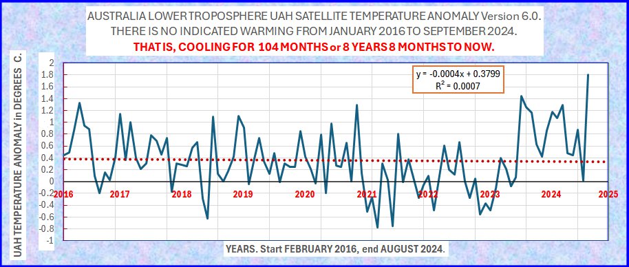
The most recent value is 1.8 degrees C, which is a record high for all time since the UAH start in December 1978.
The meaning and cause remain unclear.
To date, Australia has had less of a high peak that has been present globally and that is suspected to be related to the Hunga Tonga eruption and the large water volume it put into the stratosphere in January 2022.
This latest measurement set shows strong Southern Hemisphere warming, including over Australia.
(Thank you again, Dr Roy Spencer PhD.)
Geoff S
I show the pause starting in 2016/02 and lasting 103 months. Whatever, it’s only a month so not a big deal. Anyway, did you know that the trend is +0.51 C.decade-1 starting in 2010/07 and lasting 170 months?
Better to look at what the data actually does.
Spikes followed by cooling trends.
Explain how CO2 can do this.
Where is the evidence of human causation.
That’s easy. Just add the linear trend to the whole data set, rather than just those of the cherry-picked bits and pieces, and all will be revealed.
It’s not easy at all. To understand how a variable (e.g., temperature) changes over time, you need to account for the specific conditions under which the variable is measured.
For instance, if educational outcomes are averaged across schools with varying resources and student demographics, the resultant average probably isn’t going to reflect the true performance or needs of specific schools.
At higher altitudes, the atmosphere is much less dense compared to sea level. While the concentration of greenhouse gasses might remain constant in percentage terms, the reduced density means that the average distance a photon travels before interacting with a molecule is longer.
Why on earth would anyone expect to isolate the GHG signal, or any signal, from an average made up of measurements taken across areas with varying altitudes and physical characteristics? It’s mind-blowing.
“Why on earth would anyone expect to isolate the GHG signal, or any signal, from an average made up of measurements taken across areas with varying altitudes and physical characteristics?”
Excellent comment. That’s why the scientific frauds on here can never show us their math (along with other reasons, not least of which being that the math doesn’t exist).
When have you *ever* seen climate science provide a standard deviation for their averages? Or a kurtosis/skewness factor? If the variance of the data at different locations are different then how do you average the data without weighting the data points somehow? Since cold temps have different variance than warm temps how do you average NH and SH temps together into a “global average” without some kind of weighting scheme?
Much of climate science math is at a 3rd grade level. Just add the numbers up and find the average. Don’t worry what the numbers mean or if they are accurate at all.
As if averaging air temperature measurements across an entire country weren’t challenging enough:
Have you considered asking Dr Spencer about this yet, rather than just claiming he doesn’t understand what he’s doing?
The WMO advises using 30 years as a period of ‘climatology’.
The 30-year trend in UAH Australia currently stands at +0.16C per decade. Statistically significant warming.
Still DENYING that most of the last 23 years in Australia is made up of COOLING periods, with spike type steps between.
And still ZERO explanation or evidence of how CO2 could do that.
Squirm like the slimy little worm you are, fungal.
“The WMO advises using 30 years as a period of ‘climatology’.”
Arbitrary. Based on what?
If there is any long-term periodicity evident in the data, then the base period defining climate should be at least two or three periods. Picking a round number has no rational support.
A common “best global temperature” like 15°C would eliminate this. So would using an entire record as the baseline. I don’t think the 30 year period was picked for any other reason than to emphasize how fast things might change with a chaotic, non-linear atmosphere.
The WMO and climate science in general have sufficient annual meetings that they could easily arrive a standard global temperature to use as a baseline value for calculating ALL anomalies. The problem is that would also make their millikelvin temperature anomalies look like a joke. They could no longer say things like 0.005 ±0.001.
A metric like this would give a common base to compare temperatures to. Sadly, this would make climate science look more scientific but ruin the propaganda.
+100
They are trying to use temperature, an intensive property, as a measure of enthalpy, an extensive property. The problem is, as you note, the fact that enthalpy is not based just on temperature but on humidity and pressure as well, both of which vary widely with altitude, geography, and terrain. Yet climate science makes no attempt to weight their temperature data to account for this, not even for their daily mid-range temperature calculation.
Denying data patterns that are obvious to a blind monkey.
Hilarious..
Notice you have ZERO evidence of CO2 doing anything.
“all will be revealed.”
You have revealed that all you have is moronic brain-washed cultism, with zero scientific anything behind it.
Not understanding them is where your problem lies.
You certainly are incapable of explaining the jump followed by a period of cooling.
Your understanding and comprehension of anything is lower than that of a three toed sloth (apologies… not meant as an insult to three-toed sloths)
Even your tiny little mind must know it cannot be cause by human CO2.
You certainly have zero evidence , even if that is what your hallucinogenic drugs tell you it is.
Anyone can do that manipulation:
OMG, if you ignore what the data is actually doing and use all the spike changes..
Did you get your 5-year-old grand, grand child to do that ??
I did same as you.
You started at the up spikes, I started at the dips. Easy.
Blind is as blind does.
You are only making a FOOL of yourself.
And have got too senile to realise it.
Not only is Nick losing his capacity for rational thought in his dottage….
But he is also going totally blind.. or maybe just dim-witted and tunnel-blind.
So sad … lol !!!
Oh.
No, the cause is obvious.
The remnants of a strong persistent El Nino coupled to a strange SSW event,
Record 50C temperature increase over Antarctica to shift Australia’s weather patterns – ABC News
Neither have any possible human causation though.
Lower stratosphere high peak unexplained.
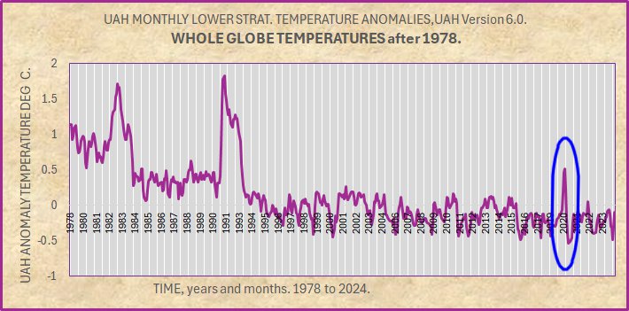
Some recent information needs to be put into context. It could be highly relevant.
For other studies, I delved into UAH lower stratosphere temperatures for the whole globe.
In simple pattern terms, there are only 3 strong excursions each showing as a high peak.
Those around years 1982 and 1991 have been researched.
Steiner et al 2020. https://doi.org/10.1175/JCLI-D-19-0998.1
Explosive volcanic eruptions such as El Chichón in
1982, Mount Pinatubo in 1991 (Robock 2000) and also
minor volcanic eruptions after 2000 affect short-term
temperature trends in the troposphere and stratosphere
(Solomon et al. 2011; Stocker et al. 2019).
Solomon 2011. https://doi.org/10.1126/science.1206027
A reasonable hypothesis would have the 2020 peak caused by volcanic eruption.
However, there would need to be a strong volcanic eruption in 2020, stronger than any since 1991, otherwise they also would show a peak for their eruption year. No such eruptions can be found by search of the literature.
The 2020 peak must therefore be attributed to another physical process.
There is not much literature as to cause in 2020. The Hunga Tonga event was 2 years later and it does not show a peak, so is easily excluded.
The Hunga Tonga simple timeline is –
“In December 2021, an eruption began on Hunga Tonga–Hunga Haʻapai, a submarine volcano in the Tongan archipelago in the southern Pacific Ocean.[6] The eruption reached a very large and powerful climax nearly four weeks later, on 15 January 2022.[7]”
https://en.wikipedia.org/wiki/2022_Hunga_Tonga%E2%80%93Hunga_Ha%CA%BBapai_eruption_and_tsunami
The main search result gives Rieger et al with their Abstract extract:
“Stratospheric aerosol, temperature, and ozone anomalies after the 2020 Australian bushfires are documented from satellite observations. Aerosol extinction is enhanced in the Southern Hemisphere (SH) lower stratosphere (LS) in early 2020, comparable in magnitude to the Calbuco eruption in 2015. Warm temperature anomalies of 1–2 K occur in the SH LS during January-April 2020 and are coincident with enhanced aerosols.”
https://agupubs.onlinelibrary.wiley.com/doi/full/10.1029/2021GL095898
…..
This does not explain the 2020 UAH peak. There have been other fires since 1978 that show no peak on the graph that can be separated from its noise.
It is plausible that this 2020 peak reflects an event that has not been noted to date.
It was a “strong” event.
If all of this is correct, we have an example of a powerful event that has affected lower stratospheric temperatures but has not yet been assigned a cause.
….
This has significant implications. Presumably (but yet to be shown) this lack of attribution could also exist for strong peaks in the troposphere.
This places a large and new uncertainty on the interpretation od UAH temperatures.
I realize you already mentioned the Australian wildfire hypothesis. Anyway, here is Dr. Spencer’s take on it.
https://www.drroyspencer.com/2020/03/australia-bushfire-smoke-now-warming-the-lower-stratosphere/
It was the Australian fires wot did it.
See aerosol graphs here ….
https://essd.copernicus.org/preprints/essd-2023-538/essd-2023-538-supplement.pdf
https://acp.copernicus.org/articles/22/9969/2022/
“More than 1 Tg smoke aerosol was emitted into the atmosphere by the exceptional 2019–2020 southeastern Australian wildfires. Triggered by the extreme fire heat, several deep pyroconvective events carried the smoke directly into the stratosphere. Once there, smoke aerosol remained airborne considerably longer than in lower atmospheric layers. The thick plumes traveled eastward, thereby being distributed across the high and mid-latitudes in the Southern Hemisphere, enhancing the atmospheric opacity. “
Anthony B,
Your argument fails unless you can show that the many other big fires around the globe over the years were not big enough to cause the effect that you blame on the Aussie 2020 fires.
Geoff S
It should be obvious that the 2020 jump in temperatures is the result of the COVID industrial shutdowns reducing the anthro’ CO2 emissions. /sarc
Rather than looking just at Australia, here’s the trend across the globe.
Lots of variation, but note the range of the trends. Some places warming or cooling at multiple degrees a decade. It’s bad enough trying to make a claim based on global changes over such a short period, let alone basing it on local trends.
.
And here’s the rate of change since the start of UAH – using the same color scale.
Globally, since December 1978 the rate of warming is 0.16°C / decade.
Since February 2016 it’s 0.39°C / decade.
Warming has come only at El Nino events.. ie NOT caused by human anything.
But you know that already.
Yes, the 2023/24 El Nino released a lot of energy.
No evidence of human causation, though, is there
All he knows how to do is regurgitate averaged averages out to the milli-Kelvins.
They quote a +/- 0.2C uncertainty for UAH meaning that the averages should be shown with no more than 1 decimal digit – i.e. the tenths digit! Yet they show averages and anomalies out to the milli-kelvin. Physical scientists they are not!
Nope!
And how many times has bwx regurgitated this 0.2°C number? As if the mere quotation of it ends all discussion.
This is SAMPLING error. Actual measurement uncertainty would be additive to this. Bottom line? It’s really impossible to know actual temperature differences to better than the units digit and possibly even the tens digit. Mill-kelvin differences are just climate scientists fooling themselves – which Feynman warned against in no uncertain terms.
Just noticing it was also the warmest summer (JJA) for the contiguous USA in the UAH record.
+1.04C on average, beating the previous record of +0.79C in 2021.
SO WHAT! All apart of the continued El Nino event, helped along by HT eruption and an arrant SSW event in the Antarctic.
You know there is absolutely ZERO evidence of any human causation.. so…
stop your incredibly STUPID and childish panic over a tiny change in NATURAL weather conditions.
You make yourself look like a little girl having a panic attack over a daddy-long-legs spider.
It is totally PATHETIC. !
Just an interesting little anecdote about US temperatures on a climate-based site operating from the US.
I thought US readers might be interested in their new record warm summer temperature and I’m pretty sure WUWT wasn’t going to tell them!
As I demonstrated earlier, a monthly mean doesn’t represent physical events or conditions. But clearly, you’re on another level, using the word ‘warmest’ to describe a 3-month average. I must be missing something – please enlighten me. I’m always keen to learn from a true expert.
Here’s some weather data I collected from the Alaskan North Slope.
I can’t help but wonder if the more frequent and intense warm spells in December 2021 had a unique impact on sea ice variations in the nearby Arctic Ocean.
But since the monthly mean for both months is identical, I guess that means the impact on sea ice extent must be exactly the same too.
No. That’s not how averages work.
You didn’t catch my sarcasm or the underlying implications.
Got it. I just wanted to make sure it was known that the average of two different samples can yield the same value even though the two samples are different.
The bigger question is whether we can truly predict the future state of the planet:
When we look closely at Bellman’s map of UAH temperature anomalies for October 2002, we notice varying anomalies depending on the region. This map is intended to provide a snapshot of the climate at that moment.
But, just as two months with the same monthly average temperature can have entirely different weather patterns and impacts, the same principle applies to the global average temperature.
The global temperature anomaly for January 24,024 might be identical to that of January 2024, but the physical state of the planet, such as the extent of polar sea ice, the position of the Intertropical Convergence Zone, Earth’s axial tilt, volcanic activity, and other factors, will almost certainly be vastly different.
Bingo, all they care about is the holy trend line.
It also highlights the perplexing nature of why TheFinalNail would use the word ‘warmest’ to describe a 3-month average, and on a more critical note, why James Hansen et al. would rely on global temperature anomalies to estimate ‘equilibrium climate sensitivity.’
Yep. Two completely different states can yield the same average value. That was my point. An example is 2023/10 and 2024/02 both of which resulted in a monthly global average temperature anomaly of +0.93 C yet the states from which that average value was computed were very different.
So you are now admitting GAT is a completely useless metric.
Good job.
You’re not missing anything. I’m pointing out that the average temperature in the US this summer was the warmest the UAH data record.
If you disagree with these figures then take it up with UAH, it’s their numbers.
Can I pick out results for the UK from this?
Yes. The August grid will be posted here in a few days.
I’ll just put this comment up for the record and we can wait to see what happens next month (4 month delay to UAH global LT temperature anomaly) and the following month (5 month delay). The Oceanic Niño Index (ONI) is one well known basis for defining El Niño/La Niña events where it reflects the rolling three-month average of sea surface temperature (SST) anomalies in the Niño-3.4 region of the equatorial Pacific Ocean. In the first figure below, the measured SST values (not the anomalies) are shown. It also shows the 30-year average SST values, which are used to compute the anomaly values.
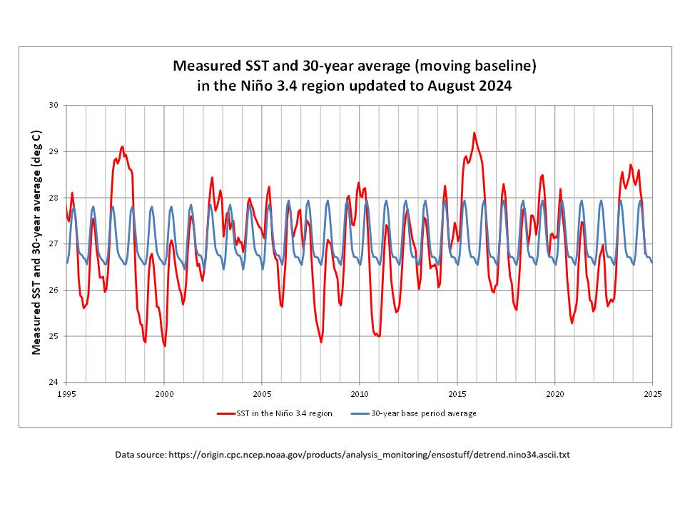
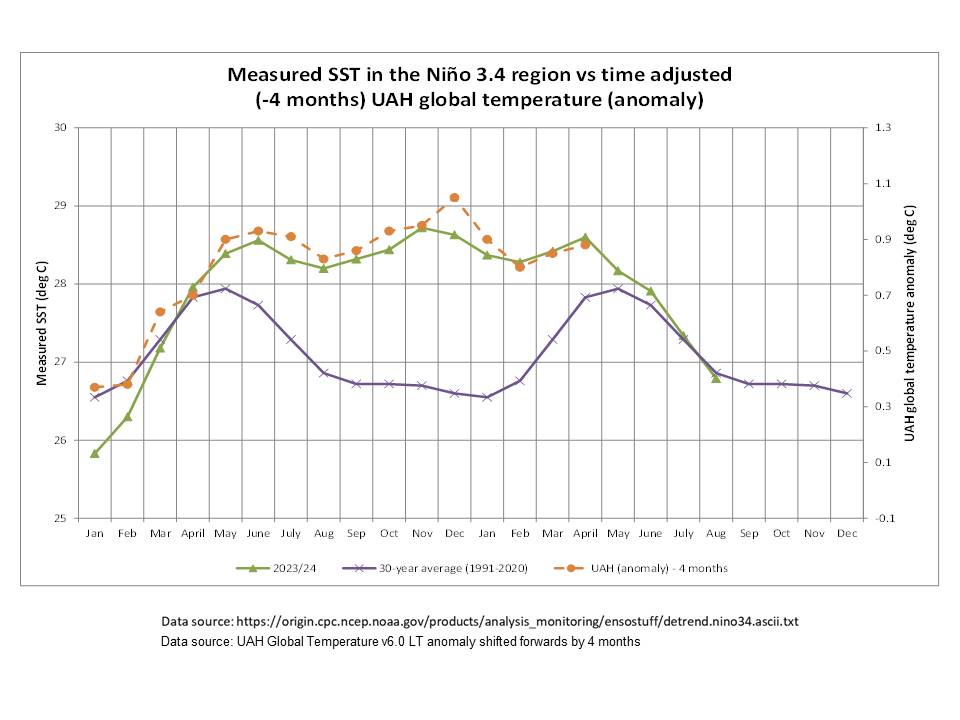
The ‘local’ SST behaviour of the very strong El Niño events (1997/1998 and 2015/2016) stand out very clearly, as does the response to the 2023/2024 event. The dominant similarities include the duration of each of these events (one year, May-May) and the fact that the raised SSTs persist for most of the event, unlike significant La Niña events which reflect a much reduced time at a minimum SST. Note that the August SST value, which is hard to see on this scale, is 26.8C, already marginally below the average for the month.
One obvious difference between the three events is the lower maximum SSTs for the recent El Niño event at around 28.5C versus 29C for the two earlier events, hence the lower ONI designation. The other difference is a bit more subtle; although the high SST duration is roughly the same, there are three distinct peaks within the recent event whereas the very strong events show one distinct SST peak, a small earlier peak, and no subsequent peak. Is this important?
In the following plot, it shows the recent SST values covering the 2023/2024 El Niño event together with the average trend. It also shows the UAH global temperature anomalies, shifted forwards by 4 months. A general delay of 4 to 5 months is well-established for global temperatures following peak ONI, so it would be interesting to see if minor variations in SST values in the Niño-3.4 region of the equatorial Pacific Ocean are also reflected in global temperatures with the same delay.
Bellman,
For simplicity, let’s focus on southeast New England, USA:
Nor’easters are common in southeast New Hampshire, forming when cold air from the north interacts with warm, moist air from the Atlantic Ocean.
The physical characteristics of nor’easters vary by season. In winter, the temperature gradient between the Arctic and the Atlantic is more pronounced. When these air masses collide, the increased atmospheric instability intensifies the storm.
In your dataset, search for temperature samples linked to this weather phenomenon and categorize them into seasonal ‘bins.’ Then, you should consider normalizing.
The entire edifice of climate science is crazy. Temperature variance is different based on season. Yet, as usual, climate science ignores this difference in variance and just jams things together with no attempt to weight the data or even to normalize it.
This is even true for some months internally, e.g. the variance of temps in the first half of August (at least here in the central US) is different from the last half of August. Yet climate science jams all the daily mid-range temps into a monthly average with no attempt to weight the data so that apples are being compared to apples.
It would make far more sense for climate science to put the data together based on the tilt angle at each step of latitude. It is this forcing that actually describes climates and climate variability. The climate models should do the same thing.
Then the station data should also be weighted based on geography and terrain. E.g. yesterday San Diego max temp was in the low 80F’s while in Ramona (30 miles inland) max temp was 100F. One is coastal and the other an inland plateau. Jamming those temps together into an average makes no physical sense at all, they are totally different climates and the variance in their temps is different.
What climate science does is similar to an HVAC engineer sizing an air conditioning unit based on the annual average temp at a location instead of on the temps during the warmest months. And yet climate science defends their methodology with religious fervor as if it was given on stone tablets found beneath a burning bush.
“Yet, as usual, climate science ignores this difference in variance and just jams things together with no attempt to weight the data or even to normalize it.”
In case you missed it, I’ve experimented with the UAH data in the way I think you are suggesting.
Here’s mad for July data, where the color indicates the deviation of temperature normalized to the standard deviation for that grid point and month, this is based on the 1991-2020 base period.
It makes it clear how unusually hot the tropics were that month. A degree or two warmer there is much more unusual than it would be in the higher latitudes.
And I then used this metric to calculate a monthly global average based on the normalized deviation for each grid point.
You totally missed the point. The ANOMALY is calculated from a baseline that has jammed data with different variances together. The monthly data for last year’s July has a different variance than the monthly data this year. And the monthly data for July from 10 years ago has a different variance than this year’s July variance.
The monthly variance is affected by the annual WEATHER each year. July in some years are wetter, some are cooler, some are warmer. Jamming them all together into a ten-year average with no weighting so you are comparing apples with apples makes no statistical sense. It’s part of the problem of trying to average an intensive property. It’s like picking up a rock in your backyard that is in sunlight at mid-day and picking one up that is in full shade of an oak tree and then averaging the two temperatures and saying that the average temperature in your backyard is that average temp. That average temp may not even exist anywhere in your backyard. It’s why Las Vegas and Miami can have the same daily mid-range temperature and vastly different climates.
It’s why enthalpy, an extensive property, is what climate science *should* be using. You *can* average extensive properties.
It’s what cymbal-monkey and others have been trying to tell you. To statisticians like you “numbers is numbers” applies to everything. It’s not a proper view of reality. The physical implications of the numbers has to be considered. And it’s not obvious what your map is telling us physically. Even worse, you haven’t included *any* indication of what the measurement uncertainty is for either the baseline or the current temps.
+100
Bellman’s maps are just images of the world with colorful blobs scattered across them.
Yes, that’s sort of how you show differences on a global scale. I tried to keep the presentation close to Spencer’s graphs – though I think his scales a little absurd.
If you want a less colorful graph you only have to download the data and produce your own.
Do what I said:
Start by gathering data tied to specific meteorological phenomena from a regional database, then organize it into seasonal bins and normalize the bins.
This way, you’re actually tracking a physical component.
It’s a far better method than simply averaging numbers over 30 or 31 days and then doing a bunch of useless calculations.
You can do that using the grids Dr. Spencer provides. That’s what they’re there for. That is if there is an analysis that is more useful to you then you are encouraged to do it using the grids provided. Dr Spencer, Bellman, myself, etc. cannot possibly anticipate all the useful ways to analyze the data and so the onerous is on you to perform this task.
Yes I get what you are saying. And there may be good uses for such an index. But, I can’t see it being popular here with the “anomalies are fraudulent” brigade.
The main problem with normalising temperatures with regard to weather conditions is that it won’t take into account changes in the frequency of weather conditions. You could have a Simpson’s paradox where everywhere looked like it was getting warmer, despite the actual average temperatures cooling. Or vice versa. This could happen if you were seeing cold and hot weather phenomena are getting warmer, but there’s been a big increase in the frequency of cold weather phenomena.
Before calculating an average based on normalized deviations, you should first disaggregate the data and analyze variance on a much more granular scale. For instance, as TG pointed out, the variance of temperature across the Central USA in August differs depending on the specific time within the month.
And as you mentioned, the frequency of these weather systems are irregular, so you will have to use a dataset that spans longer than 30 years.
Read about the Great Arctic Outbreak of 1899:
https://www.weather.gov/media/bro/research/pdf/Great_Arctic_Outbreak_1899.pdf
Nice reference! Thanks!
That should say beaches not benches!
An Analysis of the “Blizzard of ’88”
This is the second time I’ve seen you align with the Gormans. I’m curious if you are also in alignment that…
…addition (+) and division (/) are equivalent?
…Σx/n equals Σx?
…Σ(a^2) equals (Σa)^2
…a/b = b?
…d(x/n)/dx =1?
…the PEMDAS rules can be ignored?
…sqrt[xy^2] = xy?
…Taylor did not intend for δq to be the uncertainty of q?
…the NIST Uncertainty Machine does is not correct?
…NIST is a heretic?
Please advise how complete your alignment is as this may help me (and others) better respond to your posts.
Who said adding and division are the same? Nobody on here!
Do uncertainties add? Of course they do.
Why do you think relative uncertainties can can’t be added to determine a combined uncertainty.
Why do you think partial differentials are used to properly weight various measurements? Relative uncertainties don’t he same thing!
Stop just throwing stuff out to see if it sticks. Show the derivation and where any of that was said.
You are just looking more and more like a clown.
He’s more of a troll than bellcurveman.
Look at his last reference. He took what TG said literally.
Duh!
The guy is a compulsive, he keeps records of what his detractors have written that go back years. Thus the “algebra error #538” stuff, in his mind these vindicate all the crazy notions he has put out.
You did here. You said “If q = Σx/n then the uncertainty of q is the uncertainty of Σx plus the uncertainty of n.”
That is not correct. Per Taylor it is uncertainty of Σx divided by n. See equation 3.18 as I explain here.
I labeled this mistake #33 for easy identification.
Refer back to algebra mistake #14. Also #6, #8, #10, #12, #13, #16, #17, and #19 also have elements of a misunderstanding of what averages are. And, of course, for years you’ve been saying (example) the uncertainty of Σx/n is the root sum square of the uncertainties of the x’s which is incorrect since root sum square is the rule you use for Σx; not Σx/n. It is yet another conflation of sums and averages.
BTW…for the lurkers…consider the implications if uncertainty of an average were truly computed using the root sum square (RSS) rule. For example, an ASOS station records the temperature every 1-minute. The typical uncertainty might be on the order of ±1 C. If you computed a daily average using each 1-minute observation you’d erroneously conclude the daily average had an uncertainty of sqrt[ 1^2 * 1440] = ±38 C or an uncertainty of the annual average of sqrt[ 1^2 * 525600 ] = ±725 C. It doesn’t even pass the sniff test.
“That is not correct. Per Taylor it is uncertainty of Σx divided by n. See equation 3.18 as I explain here.”
Nope. You’ve been given the example from Taylor.
If y = Bx where x = x1 + x2 + … + xn –> y = B * Σx
then the uncertainty of y is u(y)/y = u(x)/x.
There is *NO* “n” in that uncertainty expression anywhere.
Eq. 3.18 ẟy/y = sqrt[ (ẟx/x)^2 + (ẟw/w)^2 ]
ẟw = 0 so you get ẟy/y = sqrt[ (ẟx/x)^2 ] = ẟx/x
This is exactly what Taylor says at the start of Section 3.4 in his example.
“That is, the fractional uncertainty in q = Bx (with B known exactly) is the same as that in x.”
Thus ẟq/q = ẟx/x. NO DIVISION BY “n”!
“BTW…for the lurkers…consider the implications if uncertainty of an average were truly computed using the root sum square (RSS) rule. For example, an ASOS station records the temperature every 1-minute. The typical uncertainty might be on the order of ±1 C. If you computed a daily average using each 1-minute observation you’d erroneously conclude the daily average had an uncertainty of sqrt[ 1^2 * 1440] = ±38 C or an uncertainty of the annual average of sqrt[ 1^2 * 525600 ] = ±725 C. It doesn’t even pass the sniff test.”
The uncertainty of the average *is* based on the variance of the data. The range of daily temperatures is typically very wide, meaning the variance is also. With a large variance values on either side of the average are very close to the average value – meaning a high uncertainty for what the actual average really is.
You’ve been given the following picture before. It displays what a statistician with real world experience would know intuitively. But you seem to continually ignore it.
Again, the average uncertainty is *NOT* the uncertainty of the average. The uncertainty of the average is the dispersion of the values that can reasonably be assigned to the estimated value. That dispersion is related to the variance of the data set.
Again, any statistician with real world experience would recognize from the shape of the temperature profile that the mid-range value (which is not an average) has a wide uncertainty. The max temperature is at the top of a sine wave with a broad peak meaning the dispersion of the values that could be attributed to the max temp is wide. The min temperature is at the bottom asymptote of an exponential decay which means the dispersion of values that could be attributed to the min temp is wide. So you have two components with wide intervals (i.e. uncertianty) of possible values being added – and that means that the uncertainties add just like variances add.
You can fight this all you want but it truly does make you look like a clown. The real world is not your statistical blackboard world.
It gets even worse – climate science *should* be working in Kelvin, not Celsius. That would be *real* science.
If the measurement uncertainty is +/- 1K (equivalent to +/- 1C) then the relative uncertainty at 293K (20C) is 1/273. Let’s say we have 1500 measurements per day and each one is 293K for an average of 293K. That gives us u(avg)/avg = sqrt[ (1/273)^2 * 1500 ].
u(avg)/avg = sqrt[ (.004)^2 * 1500 ] = sqrt[ (1.4e-5 * 1500) ] = sqrt[ .02]
u(avg)/avg = .14%
u(avg) = .14 * 293K = +/- 42K
+/- 42K is a totally believable measurement uncertainty over 1500 measurements, each with an uncertainty of +/- 1K
The fact that you can’t believe this is just more proof that you have absolutely no real world experience in metrology – and are totally unwilling to learn anything about metrology, instead stubbornly remaining willfully ignorant.
“+/- 42K is a totally believable measurement uncertainty over 1500 measurements, each with an uncertainty of +/- 1K”
It is at this point that the most generous interpretation is that Tim is just trolling us.
14% uncertainty for the relative uncertainty of a large number OF DIFFERENT THINGS is totally believable to anyone who understands metrology. Think about it! On the Celsius scale an uncertainty of 1C at 20C is about 5%. If your measurement uncertainty at 5C is still 1C then your relative uncertainty is 20%.It doesn’t take long with a 20% relative uncertainty to add up to a value that is greater than your actual measurement.
Blackboard statisticians like you and bdgwx want to believe that the average uncertainty is the uncertainty of the average. It isn’t!
Even if you are adding iid variables the variance grows. That’s because it’s based on Σ(x – x_bar). As the number of data points far from the average grows they contribute more to the variance than points that are close in. And as the variance grows so does the uncertainty of the average. Measurement uncertainty is no different.
Blackboard statisticians like you and bdgwx have the meme of all measurement uncertainty is random, Gaussian, and cancels so ingrained in your brains that you can’t avoid it. You keep saying you don’t think that way but it comes through in everything, ABSOLUTELY EVERYTHING, you both assert.
You two wouldn’t last a week in a lumberyard, machinist shop,. or production line using the standard deviation of the sample means as the measurement uncertainty you quote customers. Nor would you survive quoting the average uncertainty as the range of values a customer could expect to receive in the product they are purchasing.
Temperature measurements of different things are no different than a machinist turning out motor mounts for a ’56 Chevy Belair. Your customers are going to expect them to meet standards that are not based on the average uncertainty of your measurements but on the range (i.e. the variance) of possible values they might receive.
And they still have not learned the lesson of the average U.S. Air Force Pilot.
You try to hard. It’s just not convincing.
Tim says he has 1500 measurements made throughout the day all showing 20°C (or 293K if you prefer. It makes no difference).
Each measurement has an expanded uncertainty interval of ±1°C, which using the GUM definition means it’s reasonable to attribute a value of between 19 – 21°C to the actual individual temperature measurements. The average of the 1500 measurements is 20°C.
Time does some back of a cigarette packet and claims this means the uncertainty of the average is ±42°C. Because he’s a blackboard statistician who believes numbers is numbers, he never questions his logic, and just claims it’s reasonable to attribute a value of between -22°C and 62°C to the average of his 1500 measurements all made with an uncertainty of ±1°C.
Anyone who claims this is plausible is either trolling or in need of urgent help.
“Think about it! On the Celsius scale an uncertainty of 1C at 20C is about 5%.”
Just as you think it can’t get any dumber. Celsius is not an absolute scale. 1°C is not 5% of 20°C.
“It doesn’t take long with a 20% relative uncertainty to add up to a value that is greater than your actual measurement.”
Completely clueless. Aside from anything else when you add values, you have to add the absolute uncertainties, not the relative uncertainties. Tim knows that as he’s read every word of Taylor for meaning and done all the exercises.
“Blackboard statisticians like you and bdgwx want to believe that the average uncertainty is the uncertainty of the average. It isn’t!”
Trolling or dementia. So difficult to tell here. Tim keeps pointing out average uncertainty is not uncertainty of the average. We keep pointing out that we agree and that no-one is claiming they are the same. Yet he never remembers this and just keeps repeating the same mantra again and again as if it has some meaning for him.
“Even if you are adding iid variables the variance grows.”
And now he’s going to spell out again how little he understands this. He keeps equivocating on the word “adding”. If you are adding random variables, whether they are identically distributed or not, the variance of the sum is the sum of the variances. But he thinks this also means adding in the sense of mixing random variables.
And neither of these are the same as taking the average of random variables. The variance of the average of N random variables is the same of the variances divided by N². It’s from this you get the formula for the SEM.
“Blackboard statisticians like you and bdgwx have the meme of all measurement uncertainty is random, Gaussian, and cancels so ingrained in your brains that you can’t avoid it.”
See my comment about the “average uncertainty” nonsense.
“That gives us u(avg)/avg = sqrt[ (1/273)^2 * 1500 ].”
You can see why he hates “blackboard mathematicians”. He’s just hopeless at algebra. Writes down any old equation as long as it confirms his argument.
He’s adding 1500 temperature readings, so you have to add the absolute uncertainties not the relative uncertainties, as he’s doing here. Then he’s doing his usual thing of mixing up the sum and the average. He really needs to read Taylor for meaning, rather than juts making it up. Break the equation into it’s parts.
avg = sum / 1500. That’s adding and dividing so you have to do them separately.
The sum is adding so add the absolute uncertainties, ±1°C, in quadrature (if we can assume as Tim does that they are random.
u(sum) = √(1^2 * 1500) ≃ ±39°C.
Now divide sum by 1500 to get the average. Use the rules for combining uncertainties for divisions.
u(avg)/avg = u(sum)/sum + u(1500)/1500
and as the uncertainty of 1500 is zero.
u(avg) / avg = u(sum) / sum
It doesn’t actually matter what the relative uncertainties are at this point as it just rearranges to
u(avg) = u(sum) / 1500 ≃ 39 / 1500 ≃ ±0.03°C.
But if you want to use actual relative uncertainties
u(avg) / 293K = 39K / (293K * 1500) ≃ 8.9 * 10^(-5)
Hence
u(avg) = 39K / 1500K ≃ ±0.03K.
Hope that helps.
This will be my last comment on the subject this time, unless Tim says something even more colossally stupid than usual.
“He’s adding 1500 temperature readings, so you have to add the absolute uncertainties not the relative uncertainties, as he’s doing here.”
So I mistyped in my rush to get an answer posted.
u(avg) = quadrature addition of the individual uncertainties, not u(avg)/avg.
YOU STILL HAVEN’T ADDRESSED HOW VARIANCE ADDS EVEN WHEN THE DATA ELEMENTS ARE IID. YOU STILL HAVEN’T ADDRESSED HOW VARIANCE INCREASES EVERY TIME YOU ADD ANOTHER DATA ELEMENT.
You exhibit *NO* fundamental understanding of what variance actually is.
bellmean
———————————–
u(avg) / avg = u(sum) / sum
u(avg) = u(sum) / 1500
———————————–
Those are *NOT* the same. You have converted (avg)/sum into the number of data elements, i.e. “n”. The average divided by the sum will *NOT* be 1/1500!
You jumped from using relative uncertainties into trying to calculate the SEM. It’s all part of that meme of yours that all measurement uncertainty is random, Gaussian, and cancels so that the SEM is the uncertainty of the average.
YOU DON’T EVEN REALIZE THAT YOU DO IT!
“The average divided by the sum will *NOT* be 1/1500!”
When I said “unless Tim says something even more colossally stupid than usual.” I didn’t mean it as a challenge.
If the average equals the sum divided by 1500 it’s inevitably true that the average divided by the sum will be 1/1500. It’s basic algebra.
Everything else you rant about at great length is you asserting that the uncertainty of the sum is the uncertainty of the average, or sometimes asserting that that the uncertainty of the average is the variance of the population – you don’t even try to understand why those two claims are are a mutual contradiction, and both wrong.
There’s no point in explaining yet again why you are wrong – no matter how many times you try to provoke me with baseless insults and lies.
“If the average equals the sum divided by 1500 it’s inevitably true that the average divided by the sum will be 1/1500. It’s basic algebra.”
The uncertainty of the average is *NOT* the average uncertainty.
u(sum)/1500 is the AVERAGE UNCERTAINTY, not the uncertainty of the average.
You seem to be unable to grasp the concept that every time you add another element of uncertainty into the distribution the variance grows. The variance is the metric for the uncertainty of the average. As the variance grows so does the uncertainty of the average.
You can argue the average uncertainty is the uncertainty of the average but you can’t win. Even if every element in the “sum” has the very same average and variance the uncertainty of the average will not be the uncertainty of just one element. i.e. the average uncertainty. The expansion of the variance when you have multiple data elements *should* be a clue to anyone that it can’t happen that way. If it did then the variance of 1500 data elements with the exact same variance would have the variance of the combination the same as the variance of just one of the data elements. You would have just invalidated the accepted concept that VAR_total = ΣVAR_i where i goes from 1 to n.
“The uncertainty of the average is *NOT* the average uncertainty.”
And the usual deflection. Caught in a falsehood, claiming that “The average divided by the sum will *NOT* be 1/1500!“, he responds with something that is irrelevant to his claim.
“u(sum)/1500 is the AVERAGE UNCERTAINTY…”
No it isn’t. He’s had this explained to him hundreds of times, but his cognitive problems will not allow him to process the fact. So instead he resorts to writing it in capital letters. Somehow he thinks shouting a falsehood makes it more convincing.
“You seem to be unable to grasp the concept that every time you add another element of uncertainty into the distribution the variance grows.”
I can’t grasp it in the same way I can’t grasp the idea that the world is flat. It’s not true, I’ve explained why it’s not true, but Tim will never accept he;s wrong, and will never conduct any simple test that would demonstrate he’s wrong. So instead he just assumes anyone who understands how variance actually works, must be the one with a problem.
What he’s confusing is the fact that if you add (in the sense of summing) random variables, then the variance of the sum will be the sum of the variances. But he keeps mixing this up with the idea that the variance of the distribution of random variables increases as more elements are added (in the sense of mixing). On the whole the variance of the distribution is independent of the number of elements in it. Keep adding elements that are IID, and the variance will fluctuate, but will tend to the variance of the parent distribution.
“The variance is the metric for the uncertainty of the average.”
And here he hopes that by repeating a lie enough times it will become true. The variance of the distribution is not the uncertainty of the mean of the sample. All the roads he carefully avoids following lead to the conclusion that for a random sample of IID values taken from a population, the uncertainty of the mean will be given by the variance divided the sample size, or more usefully the standard deviation divided by the square root of the sample size.
“You can argue the average uncertainty is the uncertainty of the average...”
Either trolling or senility. No other options. There are only so many ways you can explain that nobody here is arguing that the average uncertainty is the uncertainty of the average, before you have to see that he is incapable of learning.
“Even if every element in the “sum” has the very same average and variance the uncertainty of the average will not be the uncertainty of just one element.”
Yet that’s exactly what he’s claiming when he says “The variance is the metric for the uncertainty of the average.”
“You would have just invalidated the accepted concept that VAR_total = ΣVAR_i where i goes from 1 to n.”
And he still can’t understand that an average is not a sum. The uncertainty of an average is not the uncertainty of the sum. This is the black hole at the center of all his arguments. He just can’t accept the stage where you divide the uncertainty of the sum by the sample size to get the uncertainty of the average.
Ok, here is proof. Look at equation 10 in the GUM. It is for the combined uncertainty of multiple elements.
u𝒸²(y) = Σ₁ᴺ(∂f/∂xᵢ)u²(xᵢ) (10)
One element
u𝒸²(y) = (∂f/∂x₁)u²(x₁)
Two elements
u𝒸²(y) = (∂f/∂x₁)u²(x₁) + (∂f/∂x₂)u²(x₂)
Three elements
u𝒸²(y) = (∂f/∂x₁)u²(x₁) + (∂f/∂x₂)u²(x₂) + (∂f/∂o₃)u²(x₃)
And so on.
Do you see how each new element adds to the uncertainty?
As I was saying in the comment, the problem is you keep confusing different uses of the word add.
If you sum up a number of values, then the variance increases.
var(X + Y) = var(X) + var(Y)
But you keep confusing this with the idea that as you add additional values to a sample, the variance of the sample increases in the same way. This argument is combined with the incorrect claim that the variance of the sample determines the uncertainty of the mean of the sample, and so use this to justify the idea that the larger the sample the less certain the average is.
It’s good to see you regard quoting the GUM as “proof” – maybe you could apply that to the fact that the standard deviation cannot be negative. But in this case all equation 10 shows is that if you sum multiple measurements, the uncertainty of the sum will increase. If the function is not summing, but averaging the equation shows that the uncertainty of the result will decrease as you add elements. That’s because the (∂f/∂x₁) values will be smaller the more elements are added. You are dividing each element by sample size to get the average hence,
(∂f/∂x₁) = 1/n
Also you missed the fact that the (∂f/∂x) values have to be squared.
One element
u𝒸²(y) = (∂f/∂x₁)²u²(x₁) = u²(x₁)
Two elements
u𝒸²(y) = (∂f/∂x₁)u²(x₁) + (∂f/∂x₂)u²(x₂) = (1/2)²u²(x₁) + (1/2)²u²(x₂)
Three elements
u𝒸²(y) = (∂f/∂x₁)u²(x₁) + (∂f/∂x₂)u²(x₂) + (∂f/∂o₃)u²(x₃)
= (1/3)²u²(x₁) + (1/3)²u²(x₂) + (1/3)²u²(x₃)
To test the idea that variance of the distribution increases as you add elements, lets use the UAH data for August 2024. I’ll take random grid points (without replacement) and seem what happens to the variance of the temperature as the number of grid points increases. (Note, I am not weighting by area). Here’s the first 20 values
As would be expected there is a lot of fluctuation with a small number of elements, given the large range of temperature across the globe. By chance the first two values were both near the equator, resulting in a high mean temperature and little variance. Then the 5th element was in the Antarctic which causes a big jump in the variance. After that the variance decreases as more elements are added and we start to get a more representative sample.
As you include many more elements, the variance settles down and tends towards the variance of the globe, around 175K² for this month.
Lets look at what happens when you add more elements. The variance of the distribution of 2 – 20 is 1098.12 using RSS. I added two more entries of 250 and 260 and the new variance using RSS is 1155.84.
It appears you are calculating an average of the means of some number of unique distributions. Moving the sum of means by dividing by 2 just shifts the distribution on the x-axis. The combined variance, i.e., the shape of the distribution does not change.
“Lets look at what happens when you add more elements.”
That’s what the graph shows.”
“The variance of the distribution of 2 – 20 is 1098.12 using RSS.”
RSS is not how you calculate variance.
RSS is not how you calculate variance.
Perhaps you should define what the column labeled “var” actually is. If it is variance, you must add them with RSS.
“RSS is not how you calculate variance.”
Exactly, so why claim you were using it to determine the variance. I’m beginning to suspect this is another one of those times where you are confusing everyone by using your own private Gorman definition of a term.
“Perhaps you should define what the column labeled “var” actually is.”
Maybe I should have been clearer, but I hoped it was obvious from the context. The var column is showing the variance of the sample up to that point. E.g. the variance in the 10th row is the variance of temperature in the first 10 rows. The variance in the 20th row is the variance of the first 20 temperatures.
This was to test your claim that variance always grows as you add more elements.
“If it is variance, you must add them with RSS.”
Do you actually have any understanding of the terms you use. Maybe you need to spell out what the Gorman definition of variance is, so we don’t confuse it with the correct definition.
You are the one that is mixed up. This is YOUR comment not mine. “RSS is not how you calculate variance.”. Here is the link.
https://wattsupwiththat.com/2024/09/02/uah-global-temperature-update-for-august-2024-0-88-deg-c/#comment-3967998
Sigh. I know I said that RSS is not how you calculate variance. I was assuming that as you repeated it without quotation marks, you were agreeing with me.
I didn’t want to assume you thought that RSS was how you calculated variance, because that would be assuming you were a even bigger fool than you usually appear.
So to be clear, you are saying that RSS is the correct way to calculate variance? If so then it makes most of our previous discussion pointless, because as so often when you use a term like “variance”, you mean something completely different to the expected use of the word.
Here is what you said.
I didn’t claim that is the correct way to calculate variance. I expected each row has a separate variance and were added directly by you. Your explanation still doesn’t say how the variance of each row is calculated. The fact that the single beginning row has a variance indicates the variance term is determined from other values.
“I expected each row has a separate variance and were added directly by you.”
The your expectation was wrong. Each row is a single value. But as always when I demonstrate why your original claim is wrong you play stupid and try top pretend you don’t understand the point.
I’ll repeat the var value in each row is the variance of the temperatures for all the rows up to and including that row. This is to illustrate your claim that each time you add an element to sample you increase the variance.
The variances were calculated using the cumvar function from the cumstats package in r.
“The fact that the single beginning row has a variance indicates the variance term is determined from other values.”
You need to get your eyes checked. The first row has a variance of “NA”, indicating there is no number.
Why don’t you check your evaluation of the partial derivatives again.
(∂f/∂x₁)
This is read as “the change in “f” with respect to “x₁” with all other variables held constant.. Do you see any mention of a reference to the number of terms here? That is entirely in your mind. What happens to “f” when “x₁” changes?
In essence, you have the derivative of “x₁” with all other variables being held constant. The derivative of “x₁” is “1”!
Lets look at:
(∂f/∂x₁)²u²(x₁) + (∂f/∂x₂)²u²(x₂) + (∂f/∂x₃)²u²(x₃)
We already did (∂f/∂x₁) = 1, and with x₂ and x₃ held constant their derivatives are “0”. The partials for (∂f/∂x₂) and (∂f/∂x₃) also = “1”.
Did you forget the meaning of partial derivatives? Partial derivatives take the derivative of each term separately while holding the other variables constant. That is why you need to specify the variable in the notation. Full derivatives take the derivative of each term in one fell swoop.
The derivative of a variable with an exponent of “1” is = 1. That is, x¹⁻¹⁼⁰, and x⁰ =1!
Here is a good explanation. Notice there is no 1/2 in the partial derivative of either variable for the f(x, y) = x² + y³ when there are two variables. For fun add a “z” term and see if a “1/3” appears.
https://www.mathsisfun.com/calculus/derivatives-partial.html
Your proclivity for putting 1/n in places it doesn’t belong is terribly annoying.
“Why don’t you check your evaluation of the partial derivatives again.”
What’s the point? I’ve done this dozens of times, you simply won;t accept what is a very trivial exercise.
Here. Let me find a partial derivative calculator, and see what it says.
It says the partial derivative of (x + y) / 2, with respect to x is 1/2.
https://www.symbolab.com/solver/partial-derivative-calculator/%5Cfrac%7B%5Cpartial%7D%7B%5Cpartial%20x%7D%5Cleft(%5Cfrac%7Bx%20%20%2By%7D%7B2%7D%5Cright)?or=input
It even tells you how to calculate it step by step. You try it with any number of variables, you will get the same answer.
“Do you see any mention of a reference to the number of terms here?”
When you take an average you divide the sum by the number of terms. That’s implicit tin the function of an average.
“In essence, you have the derivative of “x₁” with all other variables being held constant. The derivative of “x₁” is “1”!”
Which is why, when you add all the terms the partial derivative is 1 for each term, and the result is just the sum of the variances. But when the function is an average the function is (x1 + x2 + … + xn) / n. Hold each term constant except x1 and you get x1/n + (a load of constants). The constants contribute nothing, and you are left with x1 / n, the derivative of which is 1/n, by the Constant Multiple Rule.
Look at Dr. Taylor’s book, Page 56, Example: Measurement of q.
You can rewrite that as 2(h/t²). It doesn’t matter if you divide by 2 or multiply by 2; a constant has no uncertainty and
does not go into an combined uncertainty calculation.
The formula you are using is (1/n)(x1 + … + xn). The uncertainty equation would include u(1/2), u(x1), u(x2). The uncertainty u(1/2) = 0 and so is not included in the uncertainty calculation.
Did they never teach you proportions at school?
δh is the absolute uncertainty of the height, h is the height. δh / h is the fractional uncertainty of the height. Multiplying that by 2 and the fractional uncertainty is unchanged because 2 has no uncertainty. But 2 h is twice as big as h. Which means the absolute uncertainty from the height measurement must also be twice as big as δh, in order to preserve the fractional uncertainty.
In the example the fractional uncertainty of 2h / t² is calculated as 13.3%, mostly coming from the uncertainty of t. As g is calculated as 36.1 ft/s², which gives the uncertainty as 0.133 * 36.1 = 4.8 ft/s².
If, for some reason, the equation for g was h / t² the fractional uncertainty would still be 13.3%, but the value of g would be 46.2 / 1.6² = 18.0. Half the proper value, and so the uncertainty would be 0.133 * 18.0 = 2.4 ft/s². Half the proper uncertainty.
Why do you think Taylor is wrong in (3.9) when he says that if
q = Bx for an exact value B, then
δq = |B|δx
It requires real determination to keep ignoring this exact statement, and instead keep trying to find loopholes in examples.
You are so far out in the weeds, you’ll never find your way out. Give it up.
Look at the equation Dr. Taylor shows.
δg/g = δh/h + 2(δt/t)
Do you see a factor of 2 applied to δh/h
Look at equation 3.10
According to rule (3.10), the fractional uncertainty of t² is twice that of t. Therefore, applying the rule 3(3.8) for products and quotients to the formula g = 2h/t², we dind the fractional uncertainty
δg/g = δh/h + 2(δt/t)
I’ll say it again. The “2” in the uncertainty arises because “t” is squared and NOT FROM THE MULTIPLICATION FACTOR OF 2h!
If “t” wasn’t squared, the equation would be:
δg/g = δh/h + (δt/t)
Give some metrological resource material that supports your assertions. I tire of answering your assertions that are just your opinion of how things should work. Surely you can find something somewhere that supports you.
Pathetic. All your questions are answered in my previous comment, or by trying to understand the point of equation 10, which was where this started. Remember claimed I was wrong about the partial derivative, I provided evidence I was right – and rather than accept that you change the subject by trying to find an example you can again misunderstand.
“Do you see a factor of 2 applied to δh/h”
Once again – the factor 2 is not applied to the fractional uncertainty. The fractional uncertainty remains the same regardless of the size of h. But this means that if you scale h, you also have to scale δh in order for the fractional uncertainty to stay the same. In this example h is 46.2 ft, and δh is 0.3ft. This means that δh/h = 0.3 / 46.2 ≃ 0.7%.
The 0.7% is the fractional uncertainty. And this means that when you put 2h = 92.4 into the equation the fractional uncertainty gives you 0.7% * 92.4 = 0.6 ft. That is the absolute uncertainty of 2h that is contributing to the final absolute uncertainty.
As I say, it’s just a question of understanding how proportions work.
δh/h = (2δh)/(2h).
“Look at equation 3.10”
Why don’t you look at equation 3.9, which the one that is relevant to multiplying h by 2? You know, the one called “Measured Quantity Times Exact Number”.
Equation 10 is about raising a value to a power and is thus irrelevant to 2h. It’s relevant to t², which is why the fractional uncertainty of t is doubled. One day you and your brother really need to figure out when you are talking about fractional and when you are talking about absolute uncertainties.
“Give some metrological resource material that supports your assertions.”
Taylor equation 3.9. and Taylor’s exercises 3.9 – 3.11.
GUM equation 10.
And if you still don’t accept how the general equation works when multiplying by an exact value, try to understand the first example under “simplified forms” here:
https://physics.nist.gov/cuu/Uncertainty/combination.html
ALGEBRA MISTAKE #45
Incorrect Partial Derivative Evaluation
When y = f(x1, …, xn) = (x1 + … + xn) / n as Bellman states then ∂f/∂xi = 1/n for all xi.
The intuitive way of thinking about it in this specific case (which is an easy case) is to consider how much f changes when you change xi by 1 unit. Changing xi by 1 unit changes f by 1/n units.
And the calliope continues its merry tune…
Incorrect Partial Derivative Evaluation
Did you read this page?
https://www.mathsisfun.com/calculus/derivatives-partial.html
So, ∂f/∂x = 2x
and ∂f/∂y = 3y2
In your definition, we have no exponents.
I’ve already shown that the partial derivative of a constant term is zero.
So, your equation,
y = f(x1, …, xn) = (x1 + … + xn) / n
Turns into y = (1/n)(x1, …, xn)
And the derivative of a constant, in this case “1/n” is “0”. So, as Dr. Taylor says, “1/n” falls out of the calculation for uncertainty.
Funny, you tried this nonsense on me a few comments back and completely ignored me directing you to an online demonstration that the partial derivative of (x + y) / 2 wrt x is 1/2.
https://www.symbolab.com/solver/partial-derivative-calculator/%5Cfrac%7B%5Cpartial%7D%7B%5Cpartial%20x%7D%5Cleft(%5Cfrac%7Bx%20%20%2By%7D%7B2%7D%5Cright)
You really need to learn the difference between a result being 2x, and it being 2.
LOL at a 🤡.
You need to learn what uncertainties are and how they work. Each component in a function must have it’s uncertainty evaluated.
Your symbolab result is interesting but not pertinent.
Your function [1/2 •(x + y)] has three components.
“(1/2), (x), (y)” that must have each compnent’s uncertainty evaluated individually. A partial derivitive is simply finding the derivative of each term separately.
Put these in symbolab to see what you get.
d/dx(1/2) = 0
d/dx
Now assume (x) = 1
d/dx (y) = 1
The uncertainty is in the measurements x and y, NOT the measurement divided by “n”. Look at it this way.
Equation f(x,y) = j = (1/2)(x + y)
∂f/∂(1/2) (1/2) = 0
∂f/∂x = 1
∂f/∂y = 1
Let’s assume δx = 1.8 and δy = 1.8
So from page 79 in Dr. Taylor’s book.
δ j = √{[(∂f/∂(1/2))]δ(1/2)]² + [(∂f/∂x) δx]² + [(∂f/∂y) δy]²}
= √{0² + (1 • 1.8)² + (1 • 1.8)²} = √ = √(0 + 3.24 + 3.24) = 2.5
Now you can divide 2.5 by 2 in order to find the average uncertainty which = 1.25. But, remember what you are doing, dividing a standard deviation by 2. I’ve never seen a statistics book that says you can perform an algebraic operation like that on a variance/standard deviation and get a cogent answer.
You’re just repeating mistake #45 here.
When f(x,y) = (1/2)(x+y) then ∂f/∂x = ∂f/∂y = 1/2.
It’s hard to tell exactly what you were attempting since you got the answer wrong, but my best guess is that you may have attempted the product rule, but did it wrong. The product rule states that d(u*v)/dx = (du/dx)*v + u*(dv/dx). Note that the rules for total derivatives apply to partial derivatives as well.
Let u = 1/2 and v = x+y and f = u*v = (1/2)*(x+y)
(1) ∂f/∂x = ∂(u*v)/∂x
(2) ∂(u*v)/∂x = (∂u/∂x)*v + u*(∂v/∂x)
(3) ∂(u*v)/∂x = (∂(1/2)/∂x)*(x+y) + (1/2)*(∂(x+y)/∂x)
(4) ∂(u*v)/∂x = 0*(x+y) + (1/2)*(1 + 0)
(5) ∂(u*v)/∂x = (1/2)*(1+0)
(6) ∂(u*v)/∂x = 1/2
(7) ∂f/∂x = ∂(u*v)/∂x = 1/2
The procedure for ∂f/∂y is the same as for ∂f/∂x.
Here is the result from Wolfram Alpha [link]
The problem is in front of your keyboard.
Did posting this mess make your ego swell?
Bozo-x: self-assumed Herr Doktor Profesor of Metrology.
“Your symbolab result is interesting but not pertinent.”
Only pertinent in that it gives the correct answer to the question what is the partial derivative.
“Your function [1/2 •(x + y)] has three components.”
1/2 is just a constant.
“d/dx(1/2) = 0”
Gosh, the derivative of a constant is zero. Who’d av thunked it.
But this is not relative to the function. The partial derivative wrt x is for the function (x + x) / 2, not 1/2.
“Now assume (x) = 1
d/dx (y) = 1”
You don’t have to go to so much trouble to demonstrate you don’t understand how to do calculus.
“Equation f(x,y) = j = (1/2)(x + y)
∂f/∂(1/2) (1/2) = 0
∂f/∂x = 1
∂f/∂y = 1”
Just writing down wrong results doesn’t prove anything. The function is (1/2)(x + y), the derivatives of x and y are for that function, not some different set of functions. What do you think the f in ∂f/∂x means?
My understanding of calculus is fine. It is your lack of understanding of metrology that is sorely lacking.
Let’s go through the whole process one more time to elucidate your ignorance of uncertainty. The Eq #’s are from Dr. Taylor’s book.
1) if “q = x₁ then u(x₁) = δx₁ and:
2) If q = δx₁/w then the uncertainty is:
Now,
let’s let w =2, x₁ = 78, and δx = 1.8 we then get:
This relies on the fact that d/dx(2) = 0. In other words, stating a constant as 2 ± 0.
Now lets examine your equation of:
As I said before, you must do uncertainty term by term. You can confirm that by examining Eq. 3.18
What is the uncertainty of the “x/2” term? Well we already calculated that. It is δx. What is the uncertainty of “y/2”? Similarly, it is δy.
This is logical. What does the constant “2” contribute to the uncertainty of either the “x” term or the “y” term. Zero! A constant has no uncertainty.
Until you can convince yourself that
q = x/2 + y/2
devolves into:
δq/q = √[{((δx/x)² + (δ2/2)²] + (δy/y)² + (δ2/2)²]}
You will never understand how to calculate uncertainty. To help, ask yourself how the “1/2” contributes uncertainty to the term “x/2”.
BTW, you may not know this, but the partial differentials are only useful when the measurand has different dimensional quantities involved. That allows one to evaluate how each term affects the total. When the terms are all one dimension, there is no need for partial differentials. Simple derivatives will suffice.
“My understanding of calculus is fine”
You might want top believe that – but if you insist that the partial derivative of x/n is 1, I can tell you you are wrong.
“q = δx₁/2″
I assume you mean q = x₁/2.
”
”
And there’s your problem. q is x₁/2 = 78 / 2 = 39, hence your following lines should be
It’s fine that you make mistakes. My algebra was always pretty sloppy. But your mistakes are always serving the purpose of leading to the answer you rather than the correct answer.
You still keep ignoring Taylor (3.9) which tells you explicitly what the result of multiplying a value by an exact value will be. It’s like you just have a mental block which makes it impossible to see what you don’t want to see. As Tim keeps saying, “there’s none so blind as those who will not see.)
No mistake here. You are the one who does not understand uncertainties.
You insist on finding the average uncertainty instead of the uncertainty of the average.
You are exactly correct for one term with:
δq = 39√[(1.8/78)² = 0.9
But you realize that you have just agreed that the “1/2” has an uncertainty of zero.
So now let’s do an example of three values, each 78 ± 1.8.
Using your equation of Σxᵢ/n we get (78+78+78)/3=78 which is also:
Now let’s set up the uncertainty calculation.
This is exactly what one should expect where there is some cancelation between multiple components.
This is exactly the same as when Dr. Taylor states the coefficient of “2” in g=2h/t² has no uncertainty.
Look at Dr. Taylor’s book, Page 56, Example: Measurement of q.
The “2” is no different than the “1/2” in your equation of;
q = (1/2)(x+y) or even (1/n)(Σxᵢ)
“No mistake here.”
I’m sorry, but this drivel is wasting to much of my time. If you are not prepared to even consider why you might be mistaken you will never learn anything. I keep spelling out where you are going wrong. You never point out any mistake I might have made, you ignore my repeated attempts top get you to acknowledge Taylor 3.9. And then you just repeat the same mistakes in a slightly different form.
You are like a child trying to shove a round beg through a square hole, and lashing out at anyone who points out it will be better to try the square hole.
But let me try just one more time.
“δq/q = √{[(1.8/78)+(0/3)]² +[(1.8/78)+(0/3)]² + [(1.8/78)+(0/3)]²}”
No! No! No! When you add values, you add the absolute uncertainties not the fractional uncertainties.
“δq = 3.12”
Common sense should tell you that this is wrong.
“This is exactly what one should expect where there is some cancelation between multiple components.”
How? Each value you measured was 78 ± 1.8, implying that the true value was reasonably somewhere between 76.2 and 79.8. The sum can only reasonably be between 3*76.2 and 3*79.8. The average can therefore only reasonably be between 76.2 and 79.8. And this is assuming no cancellation. Your ±3.12 is saying you think it’s reasonable that the average can be between 74.9 and 81.1. But the only way the average could be 81.1 is if there is at least one value which was 81.1. But that would imply that the individual uncertainty was at least ±3.12.
“This is exactly the same as when Dr. Taylor states the coefficient of “2” in g=2h/t² has no uncertainty.”
You are just ignoring every other time when I and bdgwx have explained this to you. The uncertainty of 2 is zero. The impact of the number 2 is that it is making the answer twice as big and this means the same fractional uncertainty results in an absolute uncertainty that is twice as big.
There’s no more point int mew trying to explain this unless you at least acknowledge this argument, and try to explain why you think it’s wrong.
ALGEBRA MISTAKE #49
Not Following Taylor Rules Correctly.
When q = (a/x + b/y + c/z) = (t + u + v) = (78/3 + 78/3 + 78/3) you have to use both Taylor 3.16 and 3.18 to solve this problem.
Step 1
==========
Let statements
q = (a/x + b/y + c/z) = (t + u + v) = (78/3 + 78/3 + 78/3)
t = a/x, u = b/y, v = c/z
a = b = c = 78
x = y = z = 3
δa = δb = δc = 1.8
Step 2
==========
Determine δt = δ(a/x)
Use Taylor 3.18 since this is a quotient.
(1) δt/t = sqrt[ (δa/a)^2 + (δx/x)^2 ]
(2) δt/26 = sqrt[ (1.8/78)^2 + (0/3)^2 ]
(3) δt/26 = sqrt[ (0.0231)^2 + (0)^2 ]
(4) δt/26 = sqrt[ (0.000533 + 0 ]
(5) δt/26 = sqrt[ (0.000533 ]
(6) δt/26 = 0.0231
(7) δt = 26 * 0.0231
(8) δt = 0.6
It can be shown with the same procedure that δu = 0.6 and δv = 0.6 as well.
Step 3
==========
Determine δq = δ(t + u + v)
Use Taylor 3.18 since this is a sum.
(1) δq = sqrt[ δt^2 + δu^2 + δv^2 ]
(2) δq = sqrt[ 0.6^2 + 0.6^2 + 0.6^2 ]
(3) δq = sqrt[ 0.36 + 0.36 + 0.36 ]
(4) δq = sqrt[ 1.08 ]
(5) δq = 1.04
The NIST uncertainty machine confirms this result. I set a = b = c = 78 ± 1.8 and y = a/3 + b/3 + c/3. The result was 1.04 matching the result obtained by using the Taylor rules.
Your problem here was on the very first step δq/q = √{[(1.8/78)+(0/3)]² +[(1.8/78)+(0/3)]² + [(1.8/78)+(0/3)]²} which doesn’t match any Taylor rule at all.
The problem is you using the average (26). The uncertainty is in the variable “a” that equals 78 and not in the average “t” which is 26. The constant has no uncertainty and falls out of the uncertainty equations. You show the uncertainty on the right side is only in “a”. You can’t then include “3” on the left side.
If you examine his gravity example, he did not multiply either variable by the constant 2, which is equivalent to the 1/2 in you equation.
Your equation is for one measurement, technically, you need to generate a random variable with multiple measurement observations in order to assess a measurement uncertainty. Basically, something like q = {[(x1+y1+z1)/3], …, [(xn+yn+zn)/3]}. This allows the development of a probability function and an assessment of a stated value and standard deviation.
From the GUM:
I tire of trying to justify what uncertainty is when you use a funky made-up measurement equation that never exists in the real world.
Let’s discuss a real world random variable like a temperature monthly average as defined in the GUM as shown above and as done in TN 1900.
I don’t see them ever turning loose of this averaging reducing uncertainty nonsense. Air temperatures are not an instance of multiple assessments of the same variable. N was, is, and will forever remain exactly equal to one!
Their problem is in recognizing that constants disappear in an uncertainty analysis.
They just have to find an equivalent whereby uncertainty is reduced in a fashion similar to dividing by the √n.
Typo. It should be q = x₁/w.
ALGEBRA MISTAKE #48
Incorrect Multiplication
When q = x/w, x=78, and w=2 then q = 78/2 = 39.
So this step
δq/78 = √[(1.8/78)² + (0/2)²] = √[(1.8/78)² (wrong)
should be
δq/39 = √[(1.8/78)² + (0/2)²] = √[(1.8/78)² (right)
meaning
δq = 0.9
bgwxyz is a TOTAL MISTAKE.
“Now lets examine your equation of:
“What is the uncertainty of the “x/2” term? Well we already calculated that. It is δx. ”
No. You calculated it wrongly. The correct uncertainty (using Taylor 3.9, or any other method) is δx./ 2.
“This is logical.”
You’ve left it rather late to bring logic into this. The logic is simple, when you scale a value the absolute uncertainty will also have to be scaled.
“What does the constant “2” contribute to the uncertainty of either the “x” term or the “y” term”
It contributes a scaling factor. If I measure a distance on a 1:10,000 map as 23mm , with an uncertainty of 1mm. Do I expect that when I multiply it by 10,000 that I can say I know the distance is 230m with an uncertainty of ±1mm? Or should I also multiply the uncertainty by 10,000?
“Until you can convince yourself that
q = x/2 + y/2
devolves into:
δq/q = √[{((δx/x)² + (δ2/2)²] + (δy/y)² + (δ2/2)²]}”
Convince myself? I have to believe your impossible equations before I can receive true enlightenment?
δq/q = √[{((δx/x)² + (δ2/2)²] + (δy/y)² + (δ2/2)²]}
This is just wrong. You never seem to understand when you should be using relative or absolute uncertainties.
x/2 + y/2 is a sum, you use the general rule for adding x/2 top y/2, and that means you use absolute uncertainties. You need to read the parts of Taylor when he says to be careful to break up the equation into different parts to use the correct rules. In this case you can either work out the uncertainty for x/2 and y/2 separately and then apply the addition rule to add the two together, or simpler, rewrite it as (x + y) / 2. Use the adding rule to get the uncertainty of (x + y), then apply the quotient rule to divide by 2. Or much simpler, just accept the special case rule for multiplying by an exact value.
Do I really have to spoon feed you this again?
Step 1
q1 = x + y
Use summation rule
δq1 = √(δx² + δy²)
Step 2
q = q1 / 2
Use quotient rule
δq/q = √[(δq1/q1)² + (δ2 / 2)²] = δq1/q1
=>
δq = q(δq1/q1)
and as q = q1 / 2
δq = q1(δq1/q1)/2 = δq1 / 2
and expanding for q1
δq = √(δx² + δy²) / 2
” To help, ask yourself how the “1/2” contributes uncertainty to the term “x/2”.”
It might help you if you were capable of remembering all the many times I’ve explained how the 1/2 contributes, or if you could just get the algebra right and then ask yourself how it contributes. Reading Taylor’s special case for multiplication by an exact value might also help you. But that assumes you actually want to understand.
” When the terms are all one dimension, there is no need for partial differentials. Simple derivatives will suffice. ”
Nothing to do with he dimensions. If the function is linear then there is no difference between a derivative and a partial derivative for each term.
LOL! You just keep exposing your ignorance of measurments.
Dr. Taylor’s example of multiplying by an exact value supposes that one can measure a total value along with the total uncertainty. From that you can calculate an average uncertainty. The caveat is that all the sheets are exactly the same!
You fail in your assertion because the average uncertainty for a single temperature measurement at an ASOS station is 1.8°F. Guess what you get for 30 days of temperature!
1.8 • 30 = 54°F
Heck assume it is 0.5°F. That still gives a 15°F uncertainty over 30 days!
You are killing yourself with your own assertions!
“Dr. Taylor’s example of multiplying by an exact value supposes that one can measure a total value along with the total uncertainty.”
And there’s the familiar Gorman loophole argument. Having spent all this time trying to ignore the rule about multiplication by an exact value, the finally accept it but try to find a argument which they hope means it won’t work in this specific case. In this case they claim that you can only use this with a single measurement, not say a sum of measurements.
Completely absurd. The equations don;t know or care how something was measured or the uncertainty estimated. An equation cannot work for one case and not for another, unless you can demonstrate why the proof depends on the distinction.
The whole point of these rules is the propagation of errors. The point is to allow you to calculate the uncertainty for any set of operations, plugging the result of one rule as a value into another rule.
“You fail in your assertion because the average uncertainty for a single temperature measurement at an ASOS station is 1.8°F. Guess what you get for 30 days of temperature!
1.8 • 30 = 54°F”
For some reason Jim now multiplies a supposed uncertainty by 30, and claims it’s the uncertainty of a month. This would only be true if a) you assume this is a systematic error so no cancellation, and b) you are only interested in the uncertainty of the sum of 30 days worth of temperature, rather than the average.
At this point he might, but won’t reflect on why TN1900 doesn’t just add the uncertainties together, but instead divided the daily uncertainty (as defined by the standard deviation of the daily values) by the square root of the number of measurements.
Don’t you wish. That example measured the total stated value and the total uncertainty. They divided both by the number of sheets to obtain an average uncertainty PER SHEET. NOTE THE CAVEAT – EACH SHEET MUST HAVE EQUAL THICKNESS. The unstated caveat is that they must each also have the same uncertainty.
The whole rule is based upon being able to measure a collection at once with a device that has a known uncertainty. Do you have a device that will measure the entire random variable of a collection of temperatures at once? Will all the temperatures be the same? Will all the uncertainties be the same?
Look at Dr. Taylor’s derivation. It DOES NOT assume the error is systematic. It is shown as a measurement uncertainty derived from measuring a collection of objects, u𝒸(y) if you will.
You were the one that brought up Dr. Taylor’s equation for multiplying an uncertainty by a constant, not me! The calculation of 1.8 • 30 = 54°F” is exactly what multiplying an uncertainty by a constant shows. If you disagree, show the math. Otherwise learn to recognize sarcasm.
For all your self-claimed math and stats expertise, you show little compression when it comes to the physical world. You can’t even recognize when certain rules should apply. The multiplying an uncertainty by a constant requires certain assumptions be met.
Why do you think NIST TN 1900 didn’t just use a Type B uncertainty and multiply it for a combined uncertainty? Temperatures are non-repeatable events! You can find an average but the standard deviation of temperatures is just as important. It is how you know the dispersion of values surrounding the mean.
All I wish is that you were capable of trying to understand what’s being explained to you. You can derive Taylor (3.9) from any number of means, and none suggest that it only works for a simple measurement but not for a combined measurement. Assuming you are not just trolling, I feel sorry for you. You have no ability to understand how maths or logic work. You never try to understand why an equation works.
The number of things you have to misunderstand just to maintain your believe that uncertainty should increase with sample size is astonishing – how random variable are combined, how you calculate a partial derivative, how fractional uncertainties are different to absolute uncertainties, how you can use the rules pf propagation to estimate uncertainty step by step, what variance is, what Gaussian means, and so on. All this to support an assertion that is obviously nonsense – that the uncertainty of an average of things can be greater than any individual uncertainty.
“The calculation of 1.8 • 30 = 54°F” is exactly what multiplying an uncertainty by a constant shows.”
OK, I see your point now, but it’s still wrong. Multiplying an individual measurement by 30 is not the same as adding 30 independent measurements. Multiplying by 30 is equivalent to adding 30 completely dependent measurements together. Then you need equation (13) or (16) from the GUM. And see Note 1. With a simple sum of 30 values with correlation coefficients of +1, the equation reduces to a sum of all the standard uncertainties, the same as multiplying the uncertainties by 30.
“For all your self-claimed math and stats expertise, you show little compression when it comes to the physical world”
I don’t claim to have any particular expertise. Most of my understanding here has come from arguing with you. I do try to compress the physical world as little as possible though.
“The multiplying an uncertainty by a constant requires certain assumptions be met”
There are always assumptions, but in this case I can think of very few. It’s difficult to see where it would not apply – for instance it’s one of the few of the general rules that work regardless of whether the uncertainties are random or systematic. It certainly doesn’t depend on the assumptions you are claiming. If you think it depends on just a single measurement, you need to show why that would be, not just base it on the way examples are worded.
“Why do you think NIST TN 1900 didn’t just use a Type B uncertainty and multiply it for a combined uncertainty?”
That example uses exactly the same rules you say don;t apply to multiple measurements. They don’t use a Type B because they are ignoring actual measurement uncertainties, and instead treating each daily value as if it were a measurement of the mean temperature with an error. The standard deviation is an estimate of that uncertainty. Using that model you can just as easily derive the uncertainty of the average using the general rules. Just add all the values to get the sum. The uncertainty of the sum is the sum in quadrature of the daily uncertainty, i.e. the standard deviation, so the uncertainty of the sum is √22 * SD. Then take the average by dividing the sum by 22. Using Taylor’s (3.9) means dividing the uncertainty of the sum by 22, so it becomes SD / √22. Exactly the equation they use, and by no coincidence the same equation as can be used to get the SEM.
This works becasue there is no assumption in (3.9) that the value being scaled has to come from a single measurement.
You can do the same using equation 10 of the GUM, but only if you accept that the partial derivative of x/22 is 1/22.
I don’t need to show anything. The fact is that the ONLY original single measurement was of a collection of supposedly identical objects. Both the stated value and the uncertainty of that stated value was apportioned to each element of the collection. This was done to prevent having to have an extremely high-resolution device to measure each piece.
It should give you pause to think about how individual uncertainty simply adds to provide the uncertainty of the whole. No divide by “n”, no other adjustment.
It is up to you to show why the average uncertainty is the real uncertainty of a collection of temperatures rather than the sum of the parts.
Not the same thing. When dividing by 22, you are finding the average uncertainty. That is, the total uncertainty value apportioned to each individual temperature. To find the total uncertainty, you must multiply what you just divided by, i.e., end up with the uncertainty of the sum.
I don’t know how to convince you that measurement uncertainty is based upon random variables that contain a series of measurements. The statistical descriptors of that random variable are:
μ = (1/n)Σxᵢ
σ² = s²(qₖ) = [1/(n-1)]Σ(xᵢ – μ)²
Any way you cut it, σ is the standard deviation of the total distribution. You don’t see a divide by “n” again to get an individual standard deviation for each piece of data do you? This is why it is called the experimental standard deviation of the whole random variable.
As to dividing σ² by √n to achieve an experimental standard deviation of the mean, that is to find the uncertainty of the single value of μ. It is equivalent to the SEM. Dr. Taylor calls it the SDOM.
The SDOM is only applicable for repeatable measurements of the same thing. You can not justify that for temperatures. Read GUM 2.17 carefully. Then ask yourself why ISO standards require two separate uncertainties of repeatability and reproducibility.
“I don’t need to show anything.”
How convenient. Wish I could have used that answer during my exams.
“It is up to you to show why the average uncertainty is the real uncertainty of a collection of temperatures rather than the sum of the parts.”
As I keep having to say, you are either trolling or suffering from dementia at this point. The average uncertainty is not the uncertainty of the average. I’ve never claimed it was. As far as I can see the only person claiming that has been Pat Frank.
“Not the same thing.”
Really!? You don’t realize that all rules Taylor describes are derived from the general equation for error propagation?
“When dividing by 22, you are finding the average uncertainty.”
No. You are finding the average. You are then using the equation to determine the uncertainty of that average. The result of that equation is that the uncertainty is
u(avg) = √[Σu(x_i)² ] / 22
and if all uncertainties are the same size
u(avg) = u(x)² / √22
Neither of which are the average uncertainty. That would be
Σu(x_i) / 22
or
u(x)
Try to spot the difference.
“to find the total uncertainty”
Why can you never speak straight? Why do you keep bringing up undefined terms like “total uncertainty”? What do you mean by that?
“I don’t know how to convince you…”
Some suggestions. Define your terms, try to explain exactly what you are trying to achieve, try to understand what the terms you use actually mean, and try to say something that is plausible.
“…measurement uncertainty is based upon random variables that contain a series of measurements.”
See, there’s a problem straight away. random variables do not “contain” measurements. A random variable is an abstraction to describe random events. You might estimate properties of a specific variable from observations, but that does not make the observations part of the variable.
“The statistical descriptors of that random variable are:”
Some of the statistical descriptors …
“μ = (1/n)Σxᵢ”
For a finite set of outcomes the expected value (or the mean) is the weighted sum of all outcomes. For an infinite set this becomes an infinite sum. Dividing by n isn’t an option.
“σ² = s²(qₖ) = [1/(n-1)]Σ(xᵢ – μ)²”
See above. And you don’t need to divide by (n-1), a random variable isn’t a sample.
“This is why it is called the experimental standard deviation of the whole random variable.”
Nobody calls it that. The experimental standard deviation is just the sample standard deviation of your n measurements. You can then assume there is a random variable defining these measurements, with parameters estimated by that experimental set of measurements.
“As to dividing σ² by √n to achieve an experimental standard deviation of the mean, that is to find the uncertainty of the single value of μ.”
Yes. That’s what we’ve been trying to tell you for the last few years. You have a single mean for a given set of data, e.g. the average global anomaly for August 2024 was +0.88°C according to UAH. And you want to know how uncertain that single value is. (You don’t of course base this on the experimental standard deviation of the mean – it’s much more complex than that, but in general for more data it’s based on the less uncertain the result is likely to be.)
See – it wasn’t so hard to convince me.
“The SDOM is only applicable for repeatable measurements of the same thing.”
And he’s back to making up his own rules. No – just because you can use these statistical approaches for one purpose, doesn’t mean they become invalid for all other purposes. They are all based on random variables and the rules of probability. You can apply them to any applicable scenario.
You are so far off base I’m not even going to argue with you. Here are the GUM definitions, you argue with them.
4.2.1, 4.2.2, 4.2.3.
You can talk about all the mumbo jumbo of what you think statistics tells you, but these are the fundamental section that deal with a Type A evaluation.
Look at NIST TN 1900 and see what calculations NIST did to find the experimental standard deviation and the experimental standard deviation of the mean as is standard for the descriptors of a random variable. I’ll bet they meet the GUM definitions for calculating uncertainty and not yours where you recommend dividing the uncertainty by the number of values.
Read Section 4.4.3. Do you see either of the uncertainty possibilities divided by by 20?
If you can’t show a metrology reference that confirms your garbage treatment of how to develop measurement uncertainty by dividing the uncertainty by “n”, then you do not have a cogent argument. You are just waving your hands while spouting your misinformation.
I guess to someone with your understanding, hearing the correct meaning of words must seem like mumbo jumbo. All those sections of the GUM are using the term “random variable” as I and every one else does. The fact you can;t understand this is your problem. As is the fact you have to make a big deal over what was some minor correction.
“I’ll bet they meet the GUM definitions for calculating uncertainty and not yours where you recommend dividing the uncertainty by the number of values.”
They do exactly what I keep saying – divide the uncertainty of the individual measurements by the root of n. This is equivalent to adding all the individual uncertainties (i.e. the standard deviation) using quadrature to get the uncertainty of the sum, and then dividing by the number of values to get the uncertainty of the mean.
“Read Section 4.4.3. Do you see either of the uncertainty possibilities divided by by 20?”
It would be so much easier for you if you tried to understand why these equations are the way they are, rather than trying to find “gotchas” in examples.
But yes, 4.4.3 again illustrates the correct way to get the uncertainty of the mean. Work out the standard deviation of all the measurements (giving you an estimate for the uncertainty of the individual measurements), and then dividing by root 20 to get the uncertainty of the mean. Again this is equivalent to working out the uncertainty of the sum and dividing by 20.
It certainly does not show that you multiply the standard deviation by root 20. Which is what you keep arguing for. The uncertainty of the mean is less than the individual uncertainties. Something you keep denying.
“…your garbage treatment of how to develop measurement uncertainty by dividing the uncertainty by “n””
Something else that would help you is to define your terms. You keep talking about dividing the uncertainty by n – but never specify what uncertainty you think that is. This is confusing you as all the examples you give show exactly what you demand of me – metrology references that confirm my garbage treatment. It’s just you are too confused about what we are saying to see that. You fixate on the “divide by n” then claim that becasue they divide by √n that somehow proves your point. (I’m being generous in assuming you do see the divide by √n in all your examples.)
So to avoid any misunderstanding, and for future reference:
When I say divide the uncertainty by n, it’s in reference to the uncertainty of the sum of n measurements. This point came about becasue you and Tim insisted that the uncertainty of the mean was the same as the uncertainty of the sum – and I pointed out that if you are dividing the sum by n to get the average you also have to divide the uncertainty of the sum by n to get the uncertainty of the average.
This in tern leads to the well understood notion that when you add n measurements with the same random uncertainty, then the uncertainty of the sum is equal to the individual uncertainty times √n. And if you take the mean of n measurements with the same random uncertainty, then the uncertainty of the mean is equal to the individual uncertainty divided by √n.
Don’t tell me what either Tim or I have said.
By saying the bolded part of your statement, you are defying all published texts about how to find uncertainty. Read GUM 4.2.1 (Eq 3), 4.2.2 (Eq 4), 4.2.3 (Eq 5), and 4.4.3. The equations in these sections NEVER divide the standard deviations by “n” to obtain an “uncertainty of the mean”.
Uncertainties ARE DEFINED by standard deviations and not by standard deviation divided by “n”.
Look at s²(qₖ), it is divided by (n-1) already. Dividing by “n” again means you are dividing by [n(n-1)]. Show us a statistics or a metrology resource that calculates uncertainty in this fashion for an “uncertainty of the average”.
The Standard Deviation of the Mean (SDOM) “s²(q̅)” is calculated by dividing the s²(qₖ) by √n. Dividing it by “n” again to get an average SDOM is ridiculous.
Your concentration about the uncertainty of the average is crazy. Under the correct assumption, that is exactly what the SDOM provides.
“Your concentration about the uncertainty of the average is crazy. Under the correct assumption, that is exactly what the SDOM provides.”
if you would just try to read what I say, you might realise that you are agreeing with what we keep trying to tell you. The SEM/SDOM or whatever you want to call it, is the uncertainty of the mean, under the correct assumptions. And this is equal to the standard deviation of the population divided by √n. You are violently agreeing with me.
But you seem incapable if understanding that different equations can be equivalent and that some require dividing by root n, some by n, and some by n². They are still doing the same thing, just on different ways.
You really need to calm down, try to understand how algebra works, and respond to what I’m saying – for the sake of both of us.
Look at NIST TN 1900. The SD = 4.1.
According to you
Show us with the numbers from TN 1900 how you get equivalent values.
“Therefore, the √ standard uncertainty associated with the average is u(τ) = s∕ √m = 0.872 ◦C. “
4.1 / √22 ≈ 0.874°C. Same as the document allowing for rounding errors.
What do you think I did in an earlier post that you denigrated?
Rewrite that as (1/2)(x+y), then you get:
∂f/∂(1/2) (1/2) = 0
∂f/∂x (x) = 1
∂f/∂y (y) = 1
That’s funny. You do realize that gives the uncertainty of the average and not the average uncertainty. Look at Page 55 about calculating a stack of papers.
Look at a 30 day average of temperatures. Can you measure the whole month at once? Can you determine (not calculate) the total uncertainty from the device making that monthly measurement?
Now you could work backwards and say each of the individual temperatures have the same uncertainty of 1.8, therefore, the total uncertainty is 30•1.8=54! That’s what Dr. Taylor does with his sheet example.
The total uncertainty is 0.1. Each sheet has an uncertainty of 0.0005. (200)•(0.0005)=0.1! 1000 sheets would have a total uncertainty of 0.5 inches. That’s two teams of paper! Not a very good measurement to begin with.
This is now at least the 3rd time in this blog post alone that you’ve evaluated a partial derivative incorrectly.
When f(x,y) = (1/2)(x+y) then ∂f/∂x = ∂f/∂y = 1/2.
And ∂f/∂x (x) is just ∂f/∂x multiplied with x which has no relevance to this problem at all.
If you don’t know how to do partial derivatives then use a computer algebra system to do them for you.
“What do you think I did in an earlier post that you denigrated?”
Nothing like what I told you to do in the comment you quoted. As I said it’s pointless trying to keep explain this if you are unable to take any advice and just reassert your own mistakes.
“Rewrite that as (1/2)(x+y), then you get:
∂f/∂(1/2) (1/2) = 0
∂f/∂x (x) = 1
∂f/∂y (y) = 1”
Your self-believe is truly astonishing. A perfect demonstration of the Dunning–Kruger effect. I and bgdwx have not only explained repeatedly how the partial derivatives work for that function, but have shown the result using multiple online sources. Your response is to effectively say that every one else is doing it wrong.
You clearly have zero understanding of what a partial derivative is, let alone how to calculate it – yet you claim your understanding of calculus is “fine”.
A partial derivative is of a function with respect to a variable. You do not change the function if you don;t like it. You just treat all other variables as if they were constants. Your function is (1/2)(x+y). That’s the function that you have to use for the partial derivative of x and y. And that function includes the 1/2. It does not magically disappear, even if for some reason you want to treat it as a variable.
∂f/∂x (x) = 1
x is not the function. The function is (1/2)(x + y). To get the derivative with respect to x, treat why as a constant. Then the function is (1/2)x + C. C has no effect on the derivative so you just need to find the differential. ∂f/∂x for the function (1/2)x, where (1/2) is a constant. As even you must know, when you multiply a function by a constant the differential is just the differential of the function times the constant. The differential of x is 1. Multiply that by the constant (1/2) and you get
∂f/∂x = 1/2.
If you want to treat the 1/2 as a variable you can. Let’s say the function is λ(x + y). Then you still have to include it in the partial derivatives for x and y.
∂f/∂x = λ
whereas the partial derivative for λ is
∂f/∂λ = (x + y)
Hope that helps.
One final way of looking at this. Bevington page 42, on weighted sums and differences
Note the last part of that is only applicable if there is a dependency between u and v.
Now see what you get for the case a = b = 1/2.
Also regarding the idea that systematic uncertainty can cancel, Bevington goes on to say
They will generate any amount of noise to keep this garbage claim about averaging reducing “uncertainty”.
They don’t know what uncertainty is, and the bottom line is they don’t care that they don’t know.
Yep, the B&B Troll Twins, they will never understand..
ALGEBRA MISTAKE #41
Incorrect Replication of JCGM 100:2008 equation 10
The correct equation is u𝒸²(y) = Σ₁ᴺ(∂f/∂xᵢ)²u²(xᵢ) (10)
You were missing the exponent on the partial derivative.
ALGEBRA MISTAKE #42
Presumption that ∂f/∂x = 1
The partial derivative ∂f/∂x isn’t always going to equal 1. In fact, in many cases, like is the case when y = f(a, b) = (a – b) / 2, the partial derivative will be less than one thus each element adds only fractionally to the uncertainty. For y = f(a, b) = (a – b) / 2 it is the case that ∂f/∂a = ∂f/∂b = 1/2 meaning the uncertainty is less than the uncertainties u(a) and u(b).
BFD. A typing mistake.
You are doing the same false equivalence of making the calculation of a mean and the calculation of the uncertainty the same. Shame, shame.
F(a,b) = (1/2)(a + b) means you have two measurements, “a” and “b”. The uncertainty in “a” is NOT “a/2” and the same for “b”.
From Dr. Taylor’s book, Page 56, Example: Measurement of g”.
The “2” is not included in the calculation of uncertainty.
Try again.
ALGEBRA MISTAKE #43
y = (a – b) / 2 is not a mean.
I selected this measurement model intentionally to demonstrate a crucial point. That point being that the uncertainty u(y) is effectively the same as if it were a mean without it actually being a mean since you have been struggling with the understanding of what mean even is. An example use case of this measurement model is to calculate the uncertainty in the difference between two liquid volumes when a and b are in units of pints and y is in units of quarts. For example given a = 10 pints, b = 6 pints, u(a) = u(b) = 1 pint then y = (a-b)/2 = (10 pints – 6 pints) / 2 pints/quarts = 2 quarts. The uncertainty is thus u(y) = sqrt[ (∂y/∂a)^2*u(a)^2 + (∂y/∂b)*u(b)^2) ] = sqrt[ (0.5 quarts/pints)^2 * (1 pints)^2 + (0.5 quarts/pints)^2 * (1 pints)^2) ] = sqrt[ 2 * (0.5 quarts/pint)^2 * (1 pint)^2 ] = 0.7 quarts. You can verify this result with the NIST uncertainty machine.
ALGEBRA MISTAKE #44
2 is included in the calculation of uncertainty.
In regards to the example on pg. 56 of Taylor. Look at equation (3.11) for the example given. It is says δg/g = δh/h + 2δt/t. The 2 appears in g which is the denominator of the left-hand side. Remember, g = 2h/t^2.
LOL, more cherry picking with no understanding.
Let’s examine Taylor’s derivation more closely.
Rule Ed 3.10 says;
for q = xⁿ
(δq/|q|) = n (δx/|x|)
The “2” arises due to “t” being raised to the power of 2, not because of the constant “2” in the equation!
Holy cow, this is getting old!
ALGEBRA MISTAKE #46
Affirming a Disjunct
Just because you see a literal 2 in equation 3.11 on the right hand side arising as a result of t being raised to the power of 2 does not mean that the other 2 attached to h is not embedded in g appearing on the left hand side. It may be easier to see by substitution.
g = 2h/t^2
δg/g = δh/h + 2*δt/t
Therefore…
δg/(2h/t^2) = δh/h + 2*δt/t
I have boldened the 2 that you said did not exist,.
Do you hear tweety bird chirping?
GRAMMAR MISTAKE NUMBER SIX-FIFTY-SIX: COMMA ADJACENT TO PERIOD.
Nice catch. I’ll correct it now.
I have boldened the 2 that you said did not exist.
Are you going to fix your nonsense claims about cancelling systematic uncertainty?
Another lie, never posted ANYTHING of the sort.
I didn’t say it didn’t exist. I said it had no uncertainty and therefore is not included in the uncertainty calculation.
Read these again.
You have done nothing here but substitute (2h/t²) for “g”. Whoopy!
Let me show you where the “2” originates.
g=2h/t^2
δ2/2 = 0
δh/h = 0.7%
δt/t = 6.3%
δg/g = δh/h + 2*δt/t (11)
See that 2 times δt/t? That is because “t” is squared. If the factor had been t³, the uncertainty component would have been 3 times δt/t.
This is so basic it isn’t funny. I know you are trying your best to justify reducing the uncertainty but it is a lost cause.
He won’t understand, he thinks “systematic errors” have no uncertainty.
Doesn’t exist. Not included. Same thing.
Anyway the coefficient 2 attached to h is included (does exist) in the uncertainty calculation.
Let’s review
g = 2h/t^2
δg/g = δh/h + 2*δt/t
Therefore…
δg/(2h/t^2) = δh/h + 2*δt/t
Solving for δg…
δg = (2h/t^2) * (δh/h + 2*δt/t)
Are you challenging this? If so under what grounds?
δg = (2h/t^2) * (δh/h + 2*δt/t)
First – These are fractional uncertainties. They are basically percents.
Second – δg/g is a percent. (δh/h + 2*δt/t) is a percent. If you had read Taylor and understood it, you would see:
δg = (2h/t^2) * [(δh/h + 2*δt/t)/100]
So yes, the “2” is included in the calculation of the actual value of the measurand. But, the amount of the uncertainty “δg” is the value of the measurand times the percent uncertainty.
The “2” included in calculating the measurand value has zero uncertainty and is not included in the uncertainty calculation.
It is almost like you do not understand that each factor in the equation must have its uncertainty treated as a separate entity in the determination of the combined uncertainty.
For Dr. Taylor’s example, the separate values with possible uncertainty are:
“2”,
“h”,
“t²”
In your example, the values with a possible uncertainty are:
“1/2”,
“x1”,
“…”,
“xn”
Each value has its own uncertainty and must be evaluated individually. The “1/2” is a constant and has no uncertainty. Capeesh?
Maybe you don’t understand how percents are used.
You are still missing the obvious point. When you multiply something by an exact value the fractional uncertainty stays the same. Correct. No-one is disagreeing. But the consequence of that is that absolute uncertainty has to change to keep the fractional uncertainty constant. What you and Tim keep doing is mixing up these two types of uncertainty and claiming that the absolute uncertainty is unchanged.
Take Tim’s example above, where you have 1500 readings each with an absolute uncertainty of ±1K. Each reading is 293K, and you work out that the uncertainty of the sum of all these measurements is, assuming independent random uncertainty, 1 * √1500 = ±39K.
As a fractional uncertainty on the sum this is 39K / 440,000K ≃ 0.01%.
As you say, dividing the sum by 1500 to get the average does not change that fractional uncertainty. But now the uncertainty is 0.01% of 293K, or about ±0.03K.
You simply cannot say the fractional uncertainty remains unchanged, and at the same time claim the absolute uncertainty doesn’t change.
Put some numbers down.
Use the temps in NIST TN 1900. Instead of assuming no measurement uncertainty, use 0.5°C for each value in the random variable “t” and the mean is 25.6
What is δt? Do everyone a favor and show each term with its uncertainty.
Use the General Formula for Error Propagation on page 79 of Dr. Taylor’s book.
“Put some numbers down.”
I did, in the comment you are replying to. Did you not read it?
Do you really need to see numbers to understand that a percentage depends on the value it’s a percentage of? Would you sooner have 1% of $1000, or 1% of $1000000? If your answer is they are both the same as they are both 1%, maybe we could come to a business arrangement.
Perhaps you should critique Dr. Taylor’s example of Exampke: Measurement of g on Page 56. Is it correct or does it an error?
It’s correct, given it’s assumptions. Why do you think that Taylor is wrong in equation (3.9)?
“Use the temps in NIST TN 1900.”
What’s the point? If I thought that you would carefully consider the workings, and try to understand why you might be wrong, it would be worth it. But you haven’t done any such thing before.
Still,
assuming you want just the uncertainty caused by the 0.5K standard uncertainty in each maximum measurement – you have 22 measurements, and adding all the temperatures together you can use the rules for propagating uncertainties when summing, we get an uncertainty of the sum of 0.5 * √22 ≃ 2.4K.
The sum of the 22 values is about 6572K, so the fractional uncertainty is 2.4 / 6572 = 0.037%.
When we divide the sum by 22 to get the average (298.7K) we use the propagation rules quotients, so add the fractional uncertainties of the sum and 22. But as 22 is an exact number it’s uncertainty is 0, and so the fractional uncertainty of the average is equal to the fractional uncertainty of the sum.
u(avg) / avg = u(sum) / sum
that is
u(avg) / 298.7 = 0.00037
therefor,
u(avg) = 0.00037 * 298.7 = 0.11K.
This is just reiterating the special rule (3.9) that dividing the sum by 22 means we divide the absolute uncertainty of the sum by 22. That is, 2.4 / 22 = 1.1K.
Ans this in turn just gives us the common rule for averaging iid random variables SD / √N. 0.5 / √22 ≃ 0.11.
“Use the General Formula for Error Propagation on page 79 of Dr. Taylor’s book.”
What, and have people yell UNCERTAINTY IS NOT ERROR. You should be using the version from the GUM, which avoids using the word “error”.
Seriously, how many more times do I have to go through this, before you accept the answer will always be the same, and you then reject it because you don;t understand how partial differentiation works.
You have 22 values being averaged. The function is (x1 + x2 + … + x22) / 22.
You have 22 terms in the function, unless you count n as a term. But it makes no difference if you do as the uncertainty of n is 0.
The uncertainty of each term apart from n, is 0.5. The partial derivation of each term with respect to itself is 1/22.
Hence,
u(avg)² = Σ[(1/22 * x_i)²]
= Σ[(1/22)²(0.5)²]
= 22 * (1/22)² * (0.5)²
= 1/22 * 0.5²
And taking the square root of both sides
u(avg) = 1/√22 * 0.5 ≃ 0.11K
Wow.
ALGEBRA MISTAKE #47
Conflation of a Fraction with a Percent
(δh/h + 2*δt/t) is not a percent and should not be divided by 100.
And the actual value of measurand is included in the uncertainty. Therefore the 2 attached to the h is include or exists in the uncertainty of g.
Here is the math…
δg/g = δh/h + 2*δt/t
…solving for δg…
δg = g * (δh/h + 2*δt/t)
…and since g = 2h/t^2 then…
δg = (2h/t^2) * (δh/h + 2*δt/t)
δg = (2h/t^2) * [(δh/h + 2*δt/t)/100]. This correct if the values have been converted to percents as Dr. Taylor did in his example.
Example – δj / j = 0.3 cm / 20 cm = 0.015 = 1.5%
Look a Dr. Taylor’s page here.
You’ll see the fractional values converted into percents. See the blue circle.
You will see the percent divided by 100 to convert back to a decimal fraction multiplying the calculated value to find the uncertainty in the calculated value.
You know what? If it’s good enough for Dr. Taylor it is good for me too. Instead of making trite remarks, perhaps you should the time to study the subject. Doing so will make the GUM more understandable too.
He (and bellcurveman) are using Stokesian nitpicking to avoid facing the real issues.
“Unskilled and Unaware”
In the karlo marxist school there are no wrong answers in maths and any attempt to correct a pupils work is just nitpicking. All results are equal.
FIX YOUR HEAD.
“Just as you think it can’t get any dumber. Celsius is not an absolute scale. 1°C is not 5% of 20°C.”
Why do you think I used Kelvin in my analysis?
“Completely clueless. Aside from anything else when you add values, you have to add the absolute uncertainties, not the relative uncertainties. Tim knows that as he’s read every word of Taylor for meaning and done all the exercises.”
Clueless, absolutely clueless!
Taylor, Rule 3.18
ẟq/q = sqrt[ (ẟx/x)^2 + …. + (ẟw/w)^2 ]
What do you think ẟx/x represents if it isn’t the relative uncertainty?
In fact, Taylor tells you that if the magnitude of the factors in a functional relationship are different that using relative uncertainties is the only valid way to combine the measurement uncertainties. Taylor covers this in detail in Chapter 2, Sections 2.8 and 2.9 – the very start of the book!
I *HAVE* read every word of Taylor and done the exercises. It’s obvious that all you ever do is cherry pick things that you think confirm your misconceptions – while never bothering to read for understanding or working out the exercises to reinforce those understandings.
“We keep pointing out that we agree and that no-one is claiming they are the same.”
And yet you keep trying to assert that variance and measurement uncertainty doesn’t grow as you add uncertain data elements to your data set.
bellman: “Time does some back of a cigarette packet and claims this means the uncertainty of the average is ±42°C.”
If it’s not +/- 42C then WHAT IS IT?
Is it the average uncertainty of +/- 1C?
Stand up! Be BRAVE. Tell us what *YOU* think it would be! SHOW YOUR WORK!
“And neither of these are the same as taking the average of random variables. The variance of the average of N random variables is the same of the variances divided by N². It’s from this you get the formula for the SEM.”
The SEM is a metric for SAMPLING uncertainty, not for measurement uncertainty!
You have just, once more, confirmed that you *always* use the meme of “all measurement uncertainty is random, Gaussian, and cancels”. That is the *ONLY* scenario in which the SEM becomes the uncertainty of the average! It doesn’t matter how often you scream you never use that meme – it always shows up at the end in every assertion you make!
“Taylor, Rule 3.18
ẟq/q = sqrt[ (ẟx/x)^2 + …. + (ẟw/w)^2 ]
What do you think ẟx/x represents if it isn’t the relative uncertainty?”
Try reading Taylor for meaning, rather than cherry-picking. There’s a clue in the heading of that equation – “Uncertainties in Products and Quotients.” I’m talking about uncertainty when adding and subtracting values. There’s a clue in the comment you quoted – “when you add values, you have to add the absolute uncertainties, not the relative uncertainties.”. This is explained in Taylor 3.16 – “Uncertainties in Sums and Differences”.
“Try reading Taylor for meaning, rather than cherry-picking. There’s a clue in the heading of that equation – “Uncertainties in Products and Quotients.””
ROFL!! You can use relative uncertainties in ANY situation. I told you what Taylor says on the subject:
“In fact, Taylor tells you that if the magnitude of the factors in a functional relationship are different that using relative uncertainties is the only valid way to combine the measurement uncertainties. “
That fractional relationship does *NOT* have to be a quotient or division!
——————————————————–
Simpsno 260 voltmeter
Section 1.9
Item 9. *Accuracy
DC Voltage Ranges 2% of Full Scale
DC Current:
0-50uA 1.5% of FS
Others: 2% of FS
AC Voltage Ranges 3% of FS
Section 1.10
The voltage and current accuracy of this instrument is commonly expressed as a percent of full scale.This should not be confused wtih accuracy of reading (indication). For example, +2% of full scale on the 10volt range allows an error of +/- 0.20V at any point on the dial. This means that at full scale,, the accuracy reading would be +/- 2%, but at half scale it would be +/- 4%. Therefore it is advantageous to select a range which gives an indicaiton as near as possible to full scale.
————————————————————-
You just keep on demonstrating that you have absolutely no knowledge of the practice of metrology – NONE. The only cherry picking around here is yours.
“You can use relative uncertainties in ANY situation.”
You can do anything you like, you just won’t get the correct answer.
Do you have an actual quote where Taylor says you should add relative uncertainties when adding or subtracting values? Somehow I doubt it because here’s what he actually says.
Section 3.8 Propagation Step by Step
No idea why you think quoting an uncertainty as a percentage for your voltmeter is relevant. It has nothing to do with using absolute values when you add or subtract values. You just have to convert the relative values to absolute values for the specific measurements.
“Time does some back of a cigarette packet and claims this means the uncertainty of the average is ±42°C. Because he’s a blackboard statistician who believes numbers is numbers, he never questions his logic, and just claims it’s reasonable to attribute a value of between -22°C and 62°C to the average of his 1500 measurements all made with an uncertainty of ±1°C.”
You *still* don’t understand the metric of variance as it pertains to the measurement uncertainty of the average.
In order to calculate an average first you have to determine the sum of data elements. That sum *will* have a measurement uncertainty propagated from the measurement uncertainty of the individual data elements. They typical method for doing that is either direct addition of the measurement uncertainties or quadrature addition of the measurement uncertainties.
Instead of doing this method use the variance of the distribution as the uncertainty of the average. Add just two identical distributions, same average, same standard deviation, to get your sum.
You will wind up with twice the number of the same values at each data point. Since the variance is driven by (x – x_bar) those data points in the tails will add *more* to the variance than the data points close to the average. Thus the variance will grow. Meaning the uncertainty of the average will grow as well. The uncertainty of the average, as determined by the metric of variance, WILL NOT BE THE VARIANCE OF JUST ONE DATA ELEMENT BUT THE SUM OF THE VARIANCES!
This is exactly how measurement uncertainty is handled. Adding the variances is just like adding the squares of the standard deviations. When you take the square root of the sum you are, in fact, adding the standard deviations in quadrature – a well known truism in statistical analysis. If you had actually ever studied Taylor or Bevington you would recognize that this is exactly how they develop the quadrature addition of measurement uncertainties.
You don’t even realize that your ingrained meme of “all measurement uncertainty is random, Gaussian, and cancels” is driving your assertion here. If all the measurement uncertainty cancels then you can claim anything you want as being the uncertainty of the average.
You can’t even admit that variance grows when adding IID variables. You can’t even admit that variance is a metric for the uncertainty of the average.
And yet you claim that others (me specifically) are viewing measurements as “numbers is numbers”?
You are like the high school freshman learning how to calculate the length of the diagonals of a four-sided figure but has absolutely no clue as to what the length of those diagonal lengths are actually telling you!
You know by rote how to plug numbers into Excel or R to get statistical descriptors but have no idea of what those statistical descriptors are actually telling you, just like the high school student with the diagonal lengths.
Thus when Taylor says the measurement uncertainty of q in the relationship of q = Bx is u(y)/y = u(x)/x — no contribution to the measurement uncertainty from the constant B — you have absolutely no understanding of what Taylor is telling you.
That’s why you want u(y)/y to be equal to [ u(x)/x ]/ B – i.e. the average uncertainty.
Pathetic — “please support me!” — pleading for imaginary “lurkers” to back up your nonsense.
The fact remains, averaging does NOT reduce uncertainty.
And error is still not uncertainty.
He’s never addressed why variance is a metric for the uncertainty of the average and not the average measurement uncertainty. It would totally ruin his whole argument.
He tries to hide behind these inane “algebra error” claims, avoiding the real issues.
A deadly sin on bozo-x world.
Not possible.
Who are these alleged “others”?
I think I understand JG’s reference.
Consider these following dimensions:
L=∑L_k/n
W=∑W_k/n
H=∑H_k/n
Now, a pop question for you: why are these dimensions used as inputs in the measurement function f(x_1, x_2,…, x_n)?
Which reference?
Which inputs? What is the function? What is the problem being solved?
In your link, he references Type A evaluation of standard uncertainty.
I made a mistake. It should be:
Li
Wi
Hi
Actually you didn’t. What you wrote was correct for a type A evaluation. The JCGM 100:2008 nomenclature uses k as the subscript for a measurement of any x_i input measurand. See 4.1.4.
Which link? As of this posting I’ve provided 41 of them.
Are you wanting me to comment on type A evaluations in general?
Are you wanting me to comment on the scenario you defined here? If so can you add more details like how f(x_1, x_2,…, x_n) is defined? What are x_1, x_2, …, x_n and how do they related to the variables L, W, and H?
Are you wanting me to guess at how f(x_1, x_2,…, x_n) is defined? If so based on the variable names I would say L is length, W is width, and H is height. Perhaps f(x_1, x_2,…, x_n) is actually f(L, W, H) = L*W*H and computes the volume of a cube. If that is the case then per JCGM 100:2008 section 5 (type B) the uncertainty of f is u(f) = sqrt[ (WH)^2*u(L)^2 + (LH)^2*u(W)^2 + (LW)^2*u(H)^2 ] or per section 4 (type A) it is u(f) = sd[ Σ[f(L_k, W_k, H_k), k = 1 to n] / n ]. There are pros and cons of both approaches.
BTW…you can use the NIST uncertainty machine to solve for the combined uncertainty. If f(L, W, H) = L*W*H then when L = W = H = 1 m and u(L) = u(W) = u(H) = 0.1 m then f = 1 m^2 and u(f) = 0.173 m^3. If instead L = W = H = 2 m but keeping u(L) = u(W) = u(H) = 0.1 m then f = 8 m^2 and u(f) = 0.693 m^2. It’s a surprising result for some people because they erroneously think u(f) should be the same in both cases since u(L), u(W), and u(H) didn’t change. Looking above at the formula for u(f) as derived with the type B method explains why this happens. Unfortunately the explanation does require an understanding of calculus and the concept of partial derivatives.
If you feel like none of this was relevant to your question then would you mind clarifying your questions so that I might better understand what you are looking for exactly?
Let me help.
I was just going to say that without L_1, L_2,…L_N, you wouldn’t have L=∑L_k/n.
Without L=∑L_k/n, you don’t have any inputs to put into your function.
4.2.1
Equation 2: y= f(x1,x2,…,xN)
That’s your measurement model. Well technically it is an instance of the measurement model Y = f(X1,X2,…,XN) as specified in equation (1) is the actual model. Note the upper case as opposed to lower case here. Y is the output measurand while X1 through XN are the input measurands. The X’s can be anything. They can also be different (see example 4.1.1 and thus in H), Y can be used in both a type A evaluation (see 4.1.4 and 4.1.5) and a type B evaluation (see 5.1.2).
You can’t even cherry pick correctly.
Do you see the square root of the COMBINED VARIANCE? How about HAS NOT BEEN OBTAINED FROM REPEATED OBSERVATIONS?
Give it up dude. You have no training in taking measurements and evaluating them. You simply read to see something that might, and I emphasize might, be pertinent without knowing what the context is.
You want to show that you know something, fill out an uncertainty budget for a station monthly average using the following format and show it here.
These guys simply don’t understand the GUM. They have never been responsible for actual measurements and how to evaluate them.
You are repeating what I have shown them numerous times. You can have f(x1, …, xn) where each x_i is a daily temperature. And, you have a random variable [X1, …, Xn] whose mean and variance are standard calculations. Or, you can have f(x1, …, xn) become the measurand, whereby f(X1) = (x1, …, xn) / n. The problem is that f(X1) is equal to the mean, and the variance of f(X1) is the calculated using [x1, …., xn].
Every average has a distribution associated with it, ALWAYS. You can’t divide the variance of the distribution by n to get a new variance, it just doesn’t work that way.
Ultimately, it doesn’t matter how you define the function to calculate a monthly average. You still end up with the same mean “μ” and the same standard deviation “σ”. There are 30/31 pieces of data. That data forms a distribution that must be defined with statistical parameters.
You have hit the nail with your GUM references.
That’s for a type A evaluation. For a type B evaluation L can be any measurement with its associated uncertainty. For example L = 1 m and u(L) = 0.1 m are valid as inputs to f and equation 10 respectively.
H,L,W of your quantity need to be measured repeatedly, averaged, and then inserted as your input coefficients.
Thus, Type A evaluations cannot use an air temperature dataset.
Doing otherwise, the function would treat the inputs as if they were perfectly known, when in fact, the function can’t provide a meaningful estimate of the uncertainty in output y. This is because it doesn’t know how much uncertainty the inputs themselves carry.
That is one way of doing it. It’s called a type A evaluation.
Sure it can. I’ve done a type A evaluation of uncertainty on the UAH datasets in 3 different ways. 1) repeatedly sampling their grid, 2) jackknife resampling their grid, 3) repeatedly comparing their GAT with other GAT measurements.
When doing a type B evaluation you combine the known uncertainty of the inputs following the law of propagation of uncertainty. The inputs are not perfectly known. Instead they have an uncertainty already associated with them: u(L) for L, u(W) for W, and u(H) for H. Then the uncertainty of f(L, W, H) = L*W*H is u(f) = sqrt[ (WH)^2*u(L)^2 + (LH)^2*u(W)^2 + (LW)^2*u(H)^2 ].
The NIST uncertainty machine performs both a type A and type B evaluation for any measurement model you enter. For example, when I enter the measurement model y = f(L, W, H) = L*W*H then I specify L, W, H, u(L), u(W), and u(H) as inputs. I then click “Run the computation” and it will display the Monte Carlo Method (type A) results at the top and Gauss’s Formula (type B) on the bottom.
Another lie.
“Sure it can. I’ve done a type A evaluation of uncertainty on the UAH datasets in 3 different ways. 1) repeatedly sampling their grid, 2) jackknife resampling their grid, 3) repeatedly comparing their GAT with other GAT measurements.”
Malarky!
Type A uncertainty requires measuring the same thing multiple times using the same instrument under the same environmental conditions.
From the GUM:
—————————————–
4.2.1 In most cases, the best available estimate of the expectation or expected value μq of a quantity q that varies randomly [a random variable (C.2.2)], and for which n independent observations qk have been obtained under the same conditions of measurement (see B.2.15), is the arithmetic mean or average q (C.2.19) of the n observations:
B.2.15
repeatability (of results of measurements)
closeness of the agreement between the results of successive measurements of the same measurand carried out under the same conditions of measurement
—————————————————— (all bolding mine, tpg)
None of the temperature databases contain measurements that are of the same measurand carried out under the same conditions of measurement. NONE!
This has been pointed out to you over and over ad infinitum. Yet you absolutely refuse to commit it to memory.
from the GUM:
——————————————————
B.2.16
reproducibility (of results of measurements)
closeness of the agreement between the results of measurements of the same measurand carried out under changed conditions of measurement
—————————————————-(bolding mine, tpg)
The temperature databases don’t even meet the requirement for reproducibility since the same measurand is not being measured.
It doesn’t matter if you are doing statistical analysis on data being provided to you. If that data doesn’t meet the requirement for being Type A (i.e. repeatability), then it is a Type B uncertainty evaluation.
With Type A you can assume that random measurement uncertainty will cancel IF all elements of systematic bias have been eliminated or reduced to insignificance.
With temperature data not only is repeatability requirements not met, neither is the reduction of systematic bias reduced to insignificance.
All you are doing here is just confirming that to you all measurement uncertainty is random, Gaussian, and cancels – regardless of the origin of the measurement data.
With the temperature data that means you can only propagate the measurement uncertainty of the individual data elements onto the average, you can *NOT* use the SEM to evaluate the measurement uncertainty of the average. NO DIVIDING BY “N” to find the average uncertainty of the data elements. If the data elements are Type A measurements themselves then evaluate the variance of the sum of the variances. If they are Type B then either add the measurement uncertainties directly or in quadrature. For the temperature databases you will *NOT* find any measurements that actually have Type A measurement uncertainties since that would require them to have *no* systematic bias from either calibration drift or microclimate influence. And you cannot eliminate systematic bias by either homogenizing or infilling, that only spreads the systematic bias around and increases the uncertainty.
“When doing a type B evaluation you combine the known uncertainty of the inputs following the law of propagation of uncertainty. “
Temperature databases *must* be evaluated using Type B.
“Gauss’s Formula (type B) on the bottom.”
from Uncertainty Machine — User’s Manual (2013)
———————————————————————-
The GUM suggests that the Central Limit Theorem (CLT) lends support to the Gaussian approximation for the distribution of the output quantity. However, without a detailed examination of the measurement function f , and of the probability distribution of the input quantities (examinations that the GUM does not explain how to do), it is impossible to guarantee the adequacy of the Gaussian or Student’s t approximations.
The CLT states that, under some conditions, a sum of independent random variables has a probability distribution that is approximately Gaussian [Billingsley, 1979, Theorem 27.2]. The CLT is a limit theorem, in the sense that it concerns an infinite sequence of sums, and provides no indication about how close to Gaussian the distribution of a sum of a finite number of summands will be. Other results in probability theory provide such indications, but they involve more than just the means and variances that are required to apply Gauss’s formula.
—————————————————(bolding mine, tpg)
The fallacy of using Gauss’ formula on temperature databases has been continually pointed out to you yet you continue to refuse to recognize this. It may be the best that can be done using the temperature data that is available but the true measurement uncertainty is probably much larger than what it results in.
You continue to assume that the distribution of temperatures globally is a Gaussian or Student’s T WHILE NEVER JUSTIFYING THAT ASSUMPTION. And then assume that the NIST uncertainty machine gives a valid output.
Even the CLT does not provide an indication of how close to Gaussian the sample means distribution will be but you continue to assume it will be Gaussian – with no justification of the assumption.
Assuming that anomalies generated by mid-range temperatures from widely separated locations such as Montreal and Quito will form a Gaussian or Student’s T distribution would seem to be wishful thinking at best!
And since Gaussian distributions are random and symmetric around the mean, you cannot assign them to your sources of uncertainty without also accounting for systematic errors in your Type B evaluation. As we know, these systematic errors exist in the surface air temperature record, so they need to be corrected for first.
I think this is incorrect. My initial thought was that if a systematic bias is present, it not only shifts the mean of the distribution of f(x1, x2, …, xn), but also alters the distributions of the individual xi values. That’s not the case. It doesn’t change the individual xi distributions.
Of course, systematic errors still need to be corrected for, but they don’t need to be considered when assuming a distribution for xi in a Type B evaluation. Instead, the systematic errors combine with xi during the root-square-sum.
It depends on the measurement model. If y = x1 + x2 then the systematic error in x adds. If y = x1 – x2 then the systematic error in x cancels out.
The algebra here is pretty simple. Let xi = xit + xirj + xs where xit is the true value for measurand i, xirj is the random component of error for the j’th measurement of measurand i, and xs is the systematic component of error. Then when y = x1 – x2 we have y = (x1t + x1rj + xs) – (x2t + x2rj + xs) which then simplifies to y = (x1t + x1rj) – (x2t + x2rj) + (xs – xs) with the (xs – xs) being zero obviously.
This is one reason why measurements are often anomalized. It removes the systematic component of error common to all measurements.
Bullshit. You have to assume equal values for this occur. Unfortunately for you, absolutely magnitudes of systematic errors are typically unknown, and can drift with time.
Claimed by climate pseudoscientists world-wide, without evidence.
Excellent comment.
This is the fundamental core of their “all error is random, Gaussian, and cancels” mindset in which they are hopelessly mired. Without it, the entire artifice of air temperature anomalies collapses into a heap of gray ash.
This is totally unacceptable for them, so they cling to it like a boa constrictor killing prey, papering over the truth with word salad after word salad.
There is no algebra here! x1 and x2 are random variables. They have distribution as per your defintion. Their means can be averaged, but their variances add by RSS, always!
Random anything and systematic anything are standard deviations. Good grief.
You can’t simply deal with variances (uncertainties) of a random variable containing measurements by algebraically adding and subtracting their values.
V²(X + Y) = V²(X) +V²(Y) or V(X+Y) = √(V²(X) +V²(Y))
V(X – Y) = √(V²(X) +V²(Y))
Why do you think the GUM treats uncertainties as standard deviations?
Here is a graph of some summer temps I made about 3 years ago. Temps are in °C.
Lot’s of Gaussian distributions here. Santa Barbara is the only Gaussian right out the box. The Total shows what you can get with a sample size of 6 and about 60 samples. Not Gaussian, but not bad. The individual stations suck which means their uncertainties will look like TN 1900 Ex 2.
the total seems to be dominated by Santa Barbara. Santa Barbara is a coastal city so it’s not a reach to think it’s temps would be Gaussian. The other locations are inland and are multi-modal, not Gaussian at all.
You also have to remember these are histograms. What they really show is that Santa Barbara has a very small variance in temp because it is coastal and its temp is dominated by the temp of the ocean which doesn’t vary much, it’s kind of like Boston on the east coast.
I’m not sure what combining these into an “average” temp really means. Since temperature is an intensive property there really isn’t an “average” temperature across a geographical area. The biggest thing you can glean from this is the intra-seasonal temperature variation and it isn’t surprising that it is Gaussian since temps change rapidly at the start and end of summer while plateauing (i.e. lots of similar temps) during most of the summer. Tulsa and Austin are prime examples.
It is interesting to see that summer temps in Santa Barbara vary about 6C while in Charlottesville the range is about 15C. This means even the anomalies from the two locations based on temp vs time will have a similar variance. Just adding the anomalies from these two in order to create a “global” average anomaly is questionable at best, meaningless at worst. As you say, the uncertainty of the average anomaly would be significant in such a case.
,My purpose was evaluating the CLT. The sample means μ is close to the “mean of all the sample means” for what it is worth.
It is a good illustration that the CLT may give a close estimate of the mean, but the SEM by itself is not a good indicator of the variance of the population variance. The SEM is only an indicator of the interval within which the mean may lie.
As a broad brush I would estimate the sample means standard deviation ≈ 1.5. Multiplying that by the sample size of 6 gives a population standard deviation ≈ ±9 and an interval of 16 to 34. The problem is that it uses the assumption that the population distribution is normal. Fat chance!
You have no clue of what you are discussing.
1st, any kind of resampling data is not making successive measurements on the same thing. All it gives you are more counts of the same data. In other words, it gives you a higher “n”. Hell, just multiply “n” by some factor of 10 or 100
You’ll get an inflated number to divide by.
A Type A analysis requires successive measurements of the same thing under repeatable conditions. From the GUM:
Resampling existing data DOES NOT give you more new data. It just gives one a higher count of the same things.
If you read closely, the Machine expects probability distributions to be specified. The only time it will calculate them for you is when you provide the data directly to it by using the “Sample” choice.
So it does NOT perform a Type B evaluation. Have you ever seen Type B certification that comes with a device. What do you think the NOAA specs for ASOS and CRN stations are for? They put out Type B uncertainty quantities for temperature, humidity, pressure, precip, etc. in weather stations.
He won’t understand.
As others have conveyed, there are various distributions you can assign to your inputs, and the specific choice depends on the source of error and the information you have about it.
From JGCM:100:2008:
“4.3 Type B evaluation of standard uncertainty
4.3.1 For an estimate xi of an input quantity Xi that has not been obtained from repeated observations, the associated estimated variance u2(xi) or the standard uncertainty u(xi) is evaluated by scientific judgement based on all of the available information on the possible variability of Xi . The pool of information may include
Yes. I know. But that doesn’t invalidate the fact that the measurement model function y = f(x1, …, xN) can utilize inputs that are not perfectly know which was my point and which 4.3.1 confirms.
BTW…the NIST uncertainty machine handles all kinds of distributions.
No, you don’t know. If you did, you would not go around making absurd claims about how anomalies magically cancel systematic uncertainty.
You STILL don’t understand the basics, especially that error is not uncertainty, yet you pompously try to lecture people who do know these basics like you are some kind of expert.
The only ones you are fooling are your fellow ignorant trendologists, who blindly upvote your nonsense..
(bold mine)
My original statement, with the bolded words, referred to the uncertainty of xi in a measurement model during Type A evaluations, not Type B evaluations.
It seems you’re having difficulty “articulating”, (h/t bdgwx), your point once again.
: – )
“This is because it doesn’t know how much uncertainty the inputs themselves carry.”
It’s all part of their meme that “all measurement uncertainty is random, Gaussian, and cancels”. It is so ingrained in their brain that they don’t even realize when they are applying it!
In other words if a group of measurements are given as “stated value +/- measurement uncertainty” this always gets converted into “stated value” only. Only the stated values are used to determine the average and only the stated values are used to determine the SEM — ALWAYS. And they don’t even realize they do it!
If the parent distribution is (p_1 +/- u(p1), … , p_n +/- u(p_n)
assume the sample size is “a”
then sample 1 will contain elements s1_1 +/- u(s1_1), … , s1_a +/- u(s1_a)
sample 2 will contain elements s2_1 +/- u(s2_1), … s2_a +/- u(s2_a)
and so on ….
The mean of the sample 1 will be [s1_1 + … + s1_a ] / a
The uncertainty of the mean of sample 1 will be
sqrt[ u(s1_1)^2 + … + u(s1_a)^2 ]
So the mean of sample 1will be m_s1 +/- sqrt[ u(s1_1)^2 + … + u(s1_a)^2 ] –> m_s1 +/- u(s1)
mean of sample 2 will be m_s2 +/- sqrt[ u(s2_1)^2 + … + u(s2_a)^2 ] –> m_s2 +/- u(s2)
and so on.
bellman and bdgwx want to just find the SEM by dropping all the uncertainties of the means and just use the stated values (m_s1, m_s2, …, m_sa)
It’s because they always assume the measurement uncertainties, u(s1), u(s2), …. are random, Gaussian, and cancel.
AND THEY DON’T EVEN REALIZE THEY DO IT!
That is an unequivocal and indisputable violation of the Law of Propagation of Uncertainty.
Here is yet another demonstration of the absurdity of your assertion. Consider the height of males aged 20+ in the US known to within ±0.5 in. There are 124 million of us [1]. If we use your erroneous calculation we would wrongly conclude the uncertainty of the average height is ±5568 in or ±464 ft. Do you really think it is possible for the average height of an adult male in the US to approach 470 ft? Has there ever been even a single adult male in the US that approached 470 ft nevermind enough of them for the average to be 470 ft?
And again, error is not uncertainty.
When will you learn this simple fact?
“ If we use your erroneous calculation we would wrongly conclude the uncertainty of the average height is ±5568 in or ±464 ft.”
You don’t even understand what you are speaking about.
When the uncertainty overwhelms your measurements it means you need to find a better way of measuring!
It does *NOT* mean that the measurement uncertainty specifies what the maximum or minimum heights might be!
For example, use calibrated measurement devices where systematic bias is reduced to insignificant levels leaving only random uncertainty. Then make multiple measurements of each individual measurand under repeatability conditions so that a Type A uncertainty can be determined, basically the SEM of the measurements for each measurand. If that isn’t less than +/- 0.5″ then you’ll never actually know what you’ve come up with.
Then determine how large your sample size is going to be for multiple samples since you’ll never be able to measure the entire population. Then calculate the mean of each sample while propagating the uncertainties of the sample data onto that mean. Then find the mean of those sample means while also propagating the sample mean uncertainties onto the mean of the sample means.
Then quote the mean of those sample means to the same decimal digit that the uncertainty has after applying significant digit rules.
Someday you REALLY need to learn basic metrology and stop depending on Stat 101 for high school seniors.
They’ve been told this many, many times yet refuse to learn or accept reality.
It’s so cute that you think you have a point.
If you want some different analysis try doing it yourself, or explain to Dr Spencer why you think his data is wrong.
“July in some years are wetter, some are cooler, some are warmer.”
Yes, it’s called weather.
“Jamming them all together into a ten-year average with no weighting so you are comparing apples with apples makes no statistical sense.”
Nothing ever seems to make sense to you. When you average things over multiple years it’s because you want to reduce the effects of weather. Knowing that one month was different than a previous year only tells you something about the differences in the weather in those two years. Comparing two 30 year averages tells you much more about the difference in the climate.
“It’s why Las Vegas and Miami can have the same daily mid-range temperature and vastly different climates.”
You keep repeating these truisms over and over, but just keep ignoring the main point – the places can have the same temperature and different climates, but they cannot have different temperatures and the same climate. Changing temperatures over a long time is an indication of a changing climate.
“To statisticians like you”
I keep telling you that flattering though it may be, I am not a statistician. Just someone with an interest in the subject as a hobby. Just because I understand statistics enough to demonstrate your own numerous misunderstandings, does not make me a statistician, anymore than being able to explain why the Earth is not the center of the universe makes me an astronomer.
““numbers is numbers” applies to everything.”
Not to everything – but numbers are a very applicable to many situations, including things like seeing what temperatures are doing.
“The physical implications of the numbers has to be considered.”
Whoever claimed otherwise. It would be rather producing all these anomaly figures if you didn’t think they had a physical implication.
“And it’s not obvious what your map is telling us physically.”
It’s showing where, according to UAH, temperatures were warmer or colder than the temperatures for that location during the 1991-2020 period, and how unusually hot or cold they. Whether that’s a useful way of looking at the data depends on the questions you want to ask. I’m not making any claims for it’s usefulness. I just thought it might be an interesting way of looking at the data – given you were objecting to “jamming” together different anomalies whilst ignoring the variance.
“When you average things over multiple years it’s because you want to reduce the effects of weather.”
There is that “numbers is numbers” meme of statisticians and climate scientists.
WEATHER DETERMINES CLIMATE! Reducing the effects of weather means you are actually ignoring the main factor determining climate. That’s why climate science can’t tell the difference in climate between Las Vegas and Miami!
“Comparing two 30 year averages tells you much more about the difference in the climate.”
Not if you remove the effects of weather! For instance, food grains are sensitive to heat accumulation during the setting and growth of fruit. Using a mid-range daily temperature (which is *NOT* an average temperature) to analyze the climate can’t tell you *anything* about the actual climate which determines the yield of the food grain. This requires the use of a degree-day metric over the ENTIRE temperature profile, not just some hokey mid-range value.
“but they cannot have different temperatures and the same climate.”
Of course they can! This is just more “numbers is numbers” from a statistician that ignores real physical science. Have you ever heard of hardiness zones? Eastern CO, KS, the north half of OK, MO, IL are all part of the same hardiness zone but have minimum temps (F) ranging from -10:-5, -5:0, and 0:5. The entire region has basically the same climate but widely varying temps!
Again, your assertion is one made by someone that has apparently no actual life experience in reality.
” Changing temperatures over a long time is an indication of a changing climate.”
Meaning you have absolutely no understanding of what climate actually is. It’s exactly what Freeman Dyson said about climate science and their models – absolutely lacking in holistic analysis!
“Just because I understand statistics enough to demonstrate your own numerous misunderstandings”
No, what you have is the statisticians view that “numbers is numbers”. Let’s just look at the assertions you have made in this one post:
This is *all* indicative of a “numbers is numbers” meme with absolutely no understanding of physical science and reality.
“Whoever claimed otherwise. It would be rather producing all these anomaly figures if you didn’t think they had a physical implication.”
YOU HAVE SAID OTHERWISE! You said just in this post: “because you want to reduce the effects of weather.” Anomalies have *NO* physical implication without an accompanying standard deviation and measurement uncertainty. Yet *YOU* never bother with those – just like climate science doesn’t. Anomalies can’t tell you *anything* about the climate differences between Las Vegas and Miami or between McMurdo, Antarctica and Death Valley!
It’s just more “numbers is numbers” from a statistician.
“It’s showing where, according to UAH, temperatures were warmer or colder than the temperatures for that location during the 1991-2020 period”
It’s showing where someone has GUESSED at whether the temps were warmer or colder. Without the measurement uncertainty propagated onto those guesses you can’t tell if they are actual differences or just part of a guess pulled out of a crystal ball!
Excellent summary—the assertion is essentially that subtracting a 30-year baseline of some sort magically transforms weather into climate.
It don’t.
I can’t even read his rants anymore, they are pure pain.
No, subtracting a baseline turns temperature into anomaly.
You don’t need to keep pointing out that you don’t read anything I say. That’s obvious from everything you write.
/plonk/
The UAH cannot resolve the difference between San Diego and Ramona.
water vapor affects the strength of the radiation the UAH satellites will see since it will cause losses over the propagation path. The water vapor in the air over San Diego is different than the water vapor in the air over Ramona. So even if they could resolve distances less than 30 miles how would they account for the different propagation losses? If they calibrate their readings against the surface temp measurement stations at each location then they also inherit the measurement uncertainties associated with those land stations – which they seemingly always ignore just like the rest of climate science does. Meaning they can’t really distinguish temperature differences less than the tenths digit and likely in the unit digit.
Since you live in the Central USA, you’re likely aware that each tornado, for example, comes with its own unique set of circumstances—factors like size, strength, duration, and the specific atmospheric conditions that lead to its formation (i.e., humidity, temperature gradients, wind shear).
Areas directly in a tornado’s path feel its full force, while surrounding regions can experience strong winds or heavy rain from the storm system without being struck by the tornado itself.
Anyone serious about weighing their data based on variance must be extremely detail-oriented, accounting for all the variables of each storm system. My earlier example with nor’easters was just a simplified explanation; the reality is far more complex and granular.
“the reality is far more complex and granular”
Which is why climate science avoids accounting for this. It would require doing actual science, HARD won science. Far easier to just jumble a bunch of unrelated temps together and say that it means something in reality.
Being interested in New England, USA, I decided to explore how climate change has been studied in the region, focusing particularly on the methodology behind the research:
https://www.mdpi.com/2225-1154/9/12/176#B34-climate-09-00176
From the first steps in the Materials and Methods section, it’s clear what to expect.
Just as they treat their dataset as abstract figures, their Mann-Kendall test will approach the data in the same detached manner:
Do you know how many headlines from places all over the globe that are warming faster than anywhere else I have found? Geez, if you go by the headlines, the globe is actually warming faster than what the IPCC promotes!
From the chart, 1st block:
#2 inserts non-existant data
#3 assumes the measured data can actually resolve 10 mK
#4 & #5: standard deviations from these averages: ignored
Ditto for the next two blocks
Then:
#2: assume sigma/root(N) tells you everything you need to know — “error” means the error, right? DUH
NOWHERE is real measurement uncertainty used, it is assumed to be ZERO.
This is why climate science is laughed at, to include the trendology ruler monkeys who inhabit WUWT.
This is why the phrase “numbers is numbers” is so apt.
CRN stations have a Type B uncertainty of 0.3°C and ASOS 1.8°F. Temperatures in the 100ths decimal are meaningless. Temperatures should not be quoted beyond the tenths digit.
This would require:1) a working knowledge of basic experimental data handling and metrology, and 2) honesty.
(That they have to multiply stored values by 0.01 tells me it is all done with FORTRAN data statements.)
Do you think if they swapped their Figure 2 for a topographic map, they’d still ignore the standard deviations? “Numbers is numbers” indeed, LOL!
Climate scientists don’t have a clue about making measurements. They are all amateur statisticians with rudimentary knowledge of statistics.
Try and find a document that describes a measurand in detail. Describes the procedure for making measurements. What measurement model is being used. What items an uncertainty budget has and values for repeatability, reproducibility, calibration, etc. This all needs to be repeated each time a new random variable is created and previously determined uncertainty propagated forward. Instead, just wipe the whiteboard clean and start with 100% accurate numbers
Numbers is numbers.
If you are referring to [Young & Young 2021] then the answer is already no. They are not ignoring standard deviations. I counted nearly 500 references to a standard deviation or at least a concept directly related it (confidence interval, p-test, etc.)
. This is not an endorsement of the publication. MDPI is a known predatory journal publisher which means the paper may not have been adequately vetted for egregious mistakes prior to publication.
I looked at Figure 2 from the author’s work, which displays the locations of the 44 selected stations from the USHCN database.
Consider the varying elevations across these sites: two stations positioned on opposite sides of a mountain, even if close in proximity, will have different variances due to factors like orographic lift or temperature inversions.
As karlomonte pointed out regarding steps 4 and 5 of the first block, the authors neglected the standard deviations from these averages before compiling their New England regional dataset.
Statistical analysis wasn’t applied until after the univariate differencing was completed.
Yep!
They’re going to have different variances no matter what. Even if they were 1 m apart they’d have different variances.
But that’s moot because the variances you mention above arise due to weather; not measurement and so are irrelevant to the discussion of measurement uncertainty. The variance you want to consider is that arising from the act of the measurement itself if doing a type B evaluation. If doing a type A evaluation the individual variances are not needed at all. Instead you use the variance of multiple higher levels averages for comparison, jackknife resampling, or other statistical techniques to quantify the uncertainty of the higher level average.
Regardless the claim that the authors do not consider standard deviations is patently false. Actually it is absurdly false since it is mentioned nearly 500 times. You might be able to fault the authors for many things, but this is not one of them.
No, you’re wrong: they don’t take it into account when pre-processing the data. Take another look at the attached image.
And by the way, Type A evaluations, which the authors don’t even use, are meant to quantify random variations in repeated measurements.
All of their graphs contain error bars. It even says “Errors based on standard error”.
I don’t know if they do or don’t. All we know is that by the completion of the “Create annual and seasonal anomalies” the have “standard errors” for those anomalies. Did they type B it or type A it?
The image is irrelevant. It is only showing readers where the 44 USHCN stations are located. Refer to table A1 for content that is more relevant.
How do we know they didn’t type A table A1?
“Error bars” are NOT uncertainty!
Error is NOT uncertainty!
A real UA will use both!
You still just formula cherry-pick from texts you don’t understand.
“It even says “Errors based on standard error””
Measurement uncertainty ADDS to sampling uncertainty (i.e. “standard error”). Of course if it is climate science then the meme of “all measurement uncertainty is random, Gaussian, and cancels” is used to ignore that additive factor.
The mean of a sample *should* be given as “stated value +/- measurement uncertainty”. When grouping the sample means into a data set than that measurement uncertainty factor should be propagated onto the mean derived from the sample means.
But climate science never does that! Climate science only uses the stated value assuming it is 100% accurate! It’s statistical fraud.
For someone who claims not to endorse the paper, you’re certainly going out of your way to defend it.
The error bars you mentioned are applied to the anomalies in their datasets for each New England state, but that’s not the point we’re discussing. This is:
“Once the data were preprocessed, annual, and seasonal (spring, summer, fall, winter) averages and anomalies were created from the following months:
Various researchers have organized USHCN data and other temperature data sets in annual and seasonal formats specifically to reduce noise and provide a clearer signal [42,43,44]. We further reduced the noise by creating five-year and 10-year averages for the annual and seasonal data as others have done [34,45,46].
The annual and seasonal anomalies were created using the 30-year base period of 1951–1980 [47], which is near the middle of the analyzed time period. For every station’s data set, a long-term average (based on the 30-year period: 1951–1980) was created for the annual and seasonal data. The yearly anomalies were created by subtracting the long-term average from each of the yearly annual and seasonal data. The annual and seasonal anomalies from each state were averaged, providing data for all of New England. The annual and seasonal anomalies from every station for every year were then averaged into five-year (half-decade) and 10-year (decadal) data sets. The annual and seasonal data at the five-year and 10-year levels were then graphed and analyzed. Change over time for the annual and seasonal data were analyzed at the five-year and 10-year levels using a univariate differencing method [48] by subtracting the first five years (1900–1904) from the last five years (2016–2020) and the first 10 years (1900–1909) from the last 10 years (2011–2020)”
Hardly. I have reasons to be critical of the publication.
I know. What I’m telling you is that consideration of a standard deviation in their pre-processing step is not necessarily a hard requirement for creating spatial averages or assessing the uncertainty of those averages. Is it helpful? Absolutely. Can it be done another way? Absolutely.
No, that’s not what you were saying. It was obvious, but now you’ve implicitly acknowledged that you’ve been obfuscating. If you were truly sincere, this would have been the first point you raised.
Take the L.
In other words, throwing away variance in the original data because it can be recovered during later calculations! Har, har, hardy har har! When it is thrown away, it can’t be recovered, EVER!
As honest as a three-dollar bill.
That is what I’m saying. Or at least it is one of the things I’m saying.
It is never my intent to obfuscate. I’m certainly guilty of not articulating well. I’ll even be the first to admit that communicating ideas especially with text is not one of my strong points. I am learning to better communicate and organize my thoughts into text though.
The first point I raised was that [Young & Young 2021] does not ignore standard deviations because I was responding to your statement “Do you think if they swapped their Figure 2 for a topographic map, they’d still ignore the standard deviations?” I don’t think it would be sincere to quote your statement above and then make a point that didn’t apply to it.
Standard error is basically what Dr. Taylor calls Standard Error Of the Mean, or SDOM. He makes clear the conditions when this can be used for measurement uncertainty.
Chapter 5, Section 5.7, Page 147
Why does climate science use standard error (SDOM) when temperatures are non-repeatable so don’t have the same true value and probably not the same standard deviation?
It is appropriate to to again discuss repeatable (used to calculate SDOM) and reproducibile measurements.
Repeatable measurements of the same thing examples are:
Reproducible measurements of similar things are non-repeatable. Some examples are:
Repeatable measurements may be characterized by SDOM if the most important thing is followed – THE EXACT SAME THING. Without that, you move into the realm of reproducibility which is specified by SD. This doesn’t remove the need for a repeatibility uncertainty, it just means you need to obtain it via a Type B analysis.
I’ve posted this before why do your references never include this?
This would remove any doubt about proper measurement uncertainty analysis from the beginning. And remember, uncertainties add, they don’t get smaller.
Repeated measurements of the same exact thing under repeatable conditions. This can allow one to to use the SDOM as the uncertainty for repeatable conditions in an uncertainty budget for that exact same thing. However, not the next thing. The next thing must go through its own measurement uncertainty evaluation for repeatability.
Measurand’s like monthly temperature average do not meet repeatable conditions for repeatable uncertainty. Temp averages can only meet reproducibility conditions. That generally requires stating the SD as the reproducibile uncertainty, while using a Type B uncertainty for the repeatability uncertainty.
I know you probably already know this stuff but I thought it was important to reiterate this to everyone.
Well said, JG.
A lot of what JG, TG, and others say is inconsistent with established methods and procedures for quantifying uncertainty and they repeatedly commit egregious math mistakes (some so trivial that even middle school age children would spot) to justify their erroneous positions and then make yet commit more egregious math mistakes in defense of the previous ones. You can see an example of what I mean in the discussion above. It is risky to align your position with theirs. You are obviously free to align your position any way you want and thus repeat mistakes; all I can do is warn you of the error.
If you want an in depth description of how to deal with uncertainty then refer to JCGM 100:2008, NIST TN 1297, ISO 21749:2005, UKAS M3003, or equivalent literature. Use the NIST Uncertainty Machine to double check calculations.
Bullshit #1
Bullshit #2
Bullshit #3
You STILL don’t understand that error is not uncertainty, yet you think you have a handle on the subject.
You’ll notice no reference to NIST TN 1900 that focuses on temperature uncertainty for a monthly average. It hits too close to home.
No reference to NIST’s Engineering Statistical Handbook. God forbid one would learn proper calculations.
I guess I’m an “other”, heh.
A lot of what JG, TG, and others say is inconsistent with established methods and procedures for quantifying uncertainty and they repeatedly commit egregious math mistakes (some so trivial that even middle school age children would spot) to justify their erroneous positions and then make yet commit more egregious math mistakes in defense of the previous ones.
ROTFLMAO.
Dude, how come you never responded to this correcttion of YOUR dubious algebra?
Here is what you wrote.
Note the w = n
Therefore, δw = δn = 0
Consequently, (δw/w)² = (0/w)² = 0
Same problem with EQ 2. You said “Assume δn = 0”, not me. Therefore, (δn/n)^2 = (0/n)² = 0
You had a chance to correct the results but didn’t.
Finally
δ(Σx/n)/(Σx/n) = √[(δ(Σx)/Σx)^2]
And, further substitution gives:
δ(Σx/n)/(Σx/n) = δq/q and (δ(Σx)/Σx) = (δ(u)/u)
Therefore, δq/q = √(δ(u)/u)²
In essence, q = (the mean) μ of the random variable and u = the sum of all the data. And how does one evaluate the delta of the sum? Maybe by the variance?
You shouldn’t denigrate others when you are so off base!
Got it. q = Σx/n and u = Σx
Got it. δq/q = √(δ(u)/u)²
Now solve for δq and simplify the expression. You’re in the home stretch. You got this!
Nope, it’s done and you don’t even realize it.
?δq/q” is the mean of a random variable.
√(δ(u)/u)² is the deviation of the sum of data in the random variable.
These terms are exactly what we have been saying. You just don’t realize it.
“μ” is the mean of a random variable. That is “Σx/n“
“σ” is the standard deviation of that random variable around the mean. That is “(δ(Σx)/Σx)²”
You fail to realize that neither “δ(Σx)” nor “Σx” are divided by “n”. Isn’t that funny, you are just too inured into your belief that the average standard deviation (the deviation assigned equally to each data point) is the proper measurement uncertainty to use and refuse to consider anything different even though it is right before your eyes.
Go back and relearn what repeatable and reproducible measurements are.
Read these definitions from the GUM. Please note the difference I have bolded.
Tell us your definition of successive measurements and measurements that are not successive. I am interested.
Here are three links you should read.
What is Measurement Uncertainty? – Advanced Spectral Technology, Inc.
Reproducibility in Metrology – Advanced Spectral Technology, Inc.
Repeatability in Metrology – Advanced Spectral Technology, Inc.
You have yet to use these terms in your discussions. Why is that? They are general concepts and have applicability in all measurements. Show us a climate science paper that mentions these categories of determining measurement uncertainty from the very first calculation of an average daily temperature to a global anomaly value.
ALGEBRA MISTAKE #38
Incomplete solve.
In algebra when you solve for a variable it means to leave that variable and only that on one side of the equals sign. By convention it is usually the left hand side.
The equation δq/q = √(δ(u)/u)² has not yet been solved for δq. You must complete an algebraic operation to do this.
ALGEBRA MISTAKE #39
Misunderstanding of a Mean
When q = Σx/n then…
q is the arithmetic mean.
…and…
δq/q is the uncertainty of q (the mean) divided by q (the mean).
REVIEW
#33 – Do not treat a quotient (/) like addition (+) when selecting a Taylor rule.
#34 – Do not confuse the average of a sample with uncertainty.
#35 – Do not incorrectly substitute an expression into variables of a formula.
#36 – Do not ignore PEMDAS rules.
#37 – Do not contradict Taylor 2.3 in the usage of the symbol δ.
#38 – Do not leave an equation unsolved.
#39 – Do not confuse the relative uncertainty of the average with the average itself.
And the clown show continues, while the calliope is playing…
Nope, both sides are reduced to their constituent terms as you defined them. If you don’t like the results then go back and redefine your terms.
I notice you did nothing to show what terms and the substitutions were incorrect. All you have done is make up inane excuses and wave your arms just like a clown.
This is a stupid comment. Point out where the confusion occurs, don’t just suggest there is some.
You need to read Section 5 of the GUM for understanding again. Remember, the way you define the measurand as a single measurement means that Y = X₁,₀.
That is exactly what my result of your definitions proves. It shows you can not get away from the fact that uncertainty rears it head regardless of what shenanigans you try to pull
ALGEBRA MISTAKE #40
Invalid Identity
δq/q does not equal δq.
Therefore δq/q = √(δ(u)/u)² has not been solved for δq.
I showed you exactly what the mistakes were. They are all unequivocal and indisputable algebra mistakes.
Let’s review what they are.
#33 – Do not treat a quotient (/) like addition (+) when selecting a Taylor rule.
#34 – Do not confuse the average of a sample with uncertainty.
#35 – Do not incorrectly substitute an expression into variables of a formula.
#36 – Do not ignore PEMDAS rules.
#37 – Do not contradict Taylor 2.3 in the usage of the symbol δ.
#38 – Do not leave an equation unsolved.
#39 – Do not confuse the relative uncertainty of the average with the average itself.
#40 – Do not use an invalid identity like a/b = a (which is false) to justify an argument.
Let’s [tinu] not — your condescension act is fooling no one.
Have you learned that error is not uncertainty yet?
Here is what you wrote.
Are you now saying Σx/n is not the mean?
Are you saying δq is not the uncertainty in q which is the mean?
Dr. Taylor says:
Have you found a resource that refutes that?
You have screwed yourself into a rabbit hole and are now stuck.
You have inadvertently arrived at a correct answer and are too blind to recognize it.
LOL.
I’m saying it is and I’m trying to convince you of that. See algebra mistakes #34 and #39. Is this your way of accepting and correcting those mistakes?
I’m saying it is and I’m trying to convince you of that. See algebra mistake #37. Is this your way of accepting and correcting those mistakes?
I have no interest in refuting that. It seems like we’re making progress here. Let’s see if we can see it through. Based your post here I accept the definitions you provided.
q = Σx/n and u = Σx
And I accept your derivation up to this point.
δq/q = √(δ(u)/u)²
Now solve for δq and simplify the expression. You’re in the home stretch. You got this! Be mindful of algebra mistakes #38, #39, and #40. Use a compute algebra system if you need to.
Idiot.
You have yet to show an actual error in my use of your own assumptions.
Keep it up. Why don’t you show a line by line of what I did and exactly how the substitutions I did were wrong instead of just complaining about generic algebra errors.
You ran away (again) from what Jim pointed out.
No surprise.
Malarky! The only one inconsistent with established methods and procedures for METROLOGY – the science of measurement – IS YOU!.
The standard deviation of the sample means (your “standard error”) is *NOT* the established method or procedure for analyzing the accuracy of a measurement. All it can tell you is how precisely you have located the average value for the parent distribution. AND that is only true if you have multiple samples – if all you have is one sample then you have to assume the standard deviation of the single sample is a perfect match for the parent distribution. That’s an assumption you have NEVER justified for any temperature data set.
You are still caught between a rock and a hard place. Either the temperature databases are a single sample with multiple single measurements or it is a parent distribution. If the first then you have to propagate the measurement uncertainty of EACH entry onto the mean you calculate using either direct addition or quadrature addition. If the second then the standard deviation of the sample means doesn’t exist. The standard deviation of the parent distribution can be calculated directly just as the average can be. And the standard deviation of the parent distribution becomes the measurement uncertainty.
You have NEVER answered the question of whether the temperature databases are a single sample or are a parent distribution. We all know why you keep on avoiding that issue.
HUH?
You really don’t understand ANYTHING about which you lecture.
More lies, the standard deviations from all those averaging steps aren’t even calculated, WHICH JUST CLAIMED DOESN’T MATTER.
Even your hand-waving is pathetic, this is the equivalent of the Ali Shuffle.
…WHICH YOU JUST CLAIMED DOESN’T MATTER.
When you look at NIST TN 1900 Example 2 and see a ±1.8 °C measurement uncertainty at a SINGLE station for a monthly average of Tmax, it is difficult to believe that these stations have a significantly better uncertainty. And remember, this example says actual measurement uncertainty of each individual measurement is negligible. Knowing that, a 30-year baseline is also going to have a significant uncertainty.
Not even you can justify creating an anomaly by SUBTRACTING two random variables and yet NOT ADDING the variance of the two random variables. Yet climate science does exactly that.
If you want to have some credibility about uncertainty, don’t just wave your hands that it is being done correctly, show us a study that has published an uncertainty budget per ISO guidelines with appropriate entries.
Reread the GUM about Type B uncertainties. They are treated as a standard deviation and are arrived at by other means than a statistical analysis. That means in a single measurement, one must consult other information to find the correct value.
Only if a person is interested in an honest assessment of reality.
“Even if they were 1 m apart they’d have different variances.”
And because of this there should be a weighting factor applied in order to compare apples to apples instead of apples to oranges!
“But that’s moot because the variances you mention above arise due to weather; not measurement and so are irrelevant to the discussion of measurement uncertainty.”
Malarky! Just a few of the complicating factors are elevation, geography, and terrain. Which CM had already pointed out to you. Comparing coastal sites with inland sites is just one of the geographical complicating factors that is not considered at all in the analysis.
It’s nothing more than the typical “numbers is numbers” analysis that climate science is famous for. Physical reality *is* different from blackboard reality but that fact is never considered in climate science.
Liar. Go read the chart, standard deviations from all the 18,000 averages are all ignored.
And typical for a ruler monkey, you attack the messenger, Fallacy is your middle name.
More like “willful ignorance”.
There is not a single place in that paper where measurement uncertainty is even mentioned let alone analyzed.
The Mann-Kendall test is basically what I have said would be more appropriate for a global analysis. Just assign trends a +, -, or 0 and add’em all up. How each individual data element is analyzed for trend is open, I haven’t discussed that.
Establishing whether or not the trend between data points is +/-/0 *is* subject to measurement uncertainty analysis and, therefore, the total result is as well. If the difference between the two data points is less than the measurement uncertainty then the trend between the two points must be given a 0 (zero). Based on my analysis of cooling degree-days around the globe I believe that what you are going to find with such analysis is that the actual global trend will have an abundance of 0’s – meaning the actual global trend is unknown and unknowable with the data available today. Of course some points will be found to be warming and some will be found to be cooling but a global trend will be indeterminate.
OK, we had the warming, where is the crisis?
I have completely stopped paying attention to this fabricated statistic. We have all agreed a “global average temperature” is nonsensical, and regardless what the calculation produces, any differences between now and any point in time previous to now is undetectable without instruments of such sensitivity they do not yet exist, if they ever will as said differences may be truly imaginary. It means nothing to my daily life. Why bother anyway, according to [any random “expert”] who stated decisively some 20 years ago that we only have 5 years left to save the world, ergo it’s too late now to do anything about it anyway.
I will check my local thermometer before I go outside to see whether or not I need a jacket, but I see no detectable difference in how often I now need a jacket compared to 50 years ago. And yes, I am that old.
So why are we wasting effort on this pointless exercise?