By Andy May
In part 3 we discussed the relationship between changes in solar activity and climate changes. Exactly how solar changes affect climate is not understood. It isn’t the immediate change in radiation delivered to the Earth, since that is too small to have much of an effect. So, it must be how Earth’s climate system reacts to the changes. The observed impact of solar irradiance changes over the solar cycle on the climate is much larger than the change in delivered radiation can account for.[1] A likely amplifying mechanism is Earth’s convection and atmospheric circulation system. This post examines that idea. It is yet another important idea that the IPCC and AR6 ignore and brush away as unimportant, vis-à-vis global warming.
The emphasis the IPCC places on global average surface temperature and the use of the phrase “global warming” suggests that atmospheric and oceanic circulation of thermal energy are not important in discussions of global climate change. Theodore Shepherd argues that global climate is driven by thermodynamics, and only regional climate is driven by convection and atmospheric circulation.[2] He also admits that climate models are much less consistent in their predictions of precipitation than temperature, and that the difference is likely due to atmospheric circulation, which affects precipitation patterns more than temperature. Finally, he acknowledges that our understanding of atmospheric circulation is weak.
The IPCC makes much of the fact that the only way Earth gains thermal energy is through radiation that is absorbed by the atmosphere or the surface from outer space and the only way it loses energy is when radiation is emitted to outer space.[3] This is true, but the apparent corollary that movement of thermal energy from one place to another on Earth’s surface makes no difference in the overall energy imbalance, is not true. Convection and circulation largely control the residence time of the energy within the climate system.[4] When the average residence time is short, Earth cools, when the residence time is long, Earth warms.
To demonstrate this, we need to examine six critical areas of climate and geological research. The first is the areal distribution of incoming and outgoing radiation around the globe and the distribution of net radiation flux (incoming-outgoing radiation). Next, we will examine energy transport from the tropics, where there is a surplus of thermal energy, to the polar regions which have a deficit, or net loss of thermal energy to space. This thermal energy transport is called the “meridional transport” of energy. When meridional transport is strong, Earth cools, and when it is weak Earth warms. Figure 1 illustrates strong meridional flow in orange and weak (or “zonal”) flow in red.
Thirdly, tropical temperatures do not vary much over geological time because over the oceans they are limited to less than 30°C by evaporation.[5] So-called “global warming” happens almost exclusively in the higher latitudes, not in the tropics. Fourth, we examine how the temperature difference between the equator and the poles forms a characteristic equator-to-pole temperature gradient. Fifth, the equator-to-pole temperature gradient today is relatively steep, suggesting the climate of today is unusually cold. Sixth, the temperature gradient powers meridional transport, the steeper it is, all else equal, the colder the Earth is.

While the temperature gradient powers meridional transport, meridional transport has many modulators, and the gradient is only one of them. It is unclear exactly how the temperature gradient and meridional transport interact, but clearly, they are the main drivers of global climate change at all time scales.[6]
In summary, discussing annual or monthly global average surface temperature as if it represents global climate change is very misleading. Earth’s climate does not behave that way. It circulates excess energy from warmer areas with a strong greenhouse effect to colder areas that have a weak greenhouse effect. Deserts and the polar regions have a weaker greenhouse effect due to their lower humidity (water vapor is the strongest greenhouse gas[7]) and can more easily send energy to space as a result. The speed of energy transport determines whether the world warms or cools. The world is not a static uniform object that simply receives energy from the Sun and evenly emits it back into space, with a minor delay caused by greenhouse gas emissions, which seems to be how the IPCC views and models our planet’s climate.
Areal distribution of energy
The tropics (roughly 30°N to 30°S) cover half of Earth’s surface. This is the region that contains the location where the Sun is directly overhead at noon. Half of the tropics, 25% of Earth’s surface, is in daylight at any given time, and this 25% of the surface receives 62% of the solar energy that strikes Earth. This, combined with a very large tropical greenhouse effect and a low albedo,[8] creates an enormous surplus of energy in the tropics.

Because more energy is received in the tropics than is emitted to space, the excess energy must be transported elsewhere. To make the situation even more complicated, Earth has an axial tilt relative to the plane of its orbit around the Sun. The effect of this tilt is illustrated in figure 2, where the Northern Hemisphere winter net energy flux[9] profile is shown as a heavy dashed line and the Northern Hemisphere summer profile is shown as a light dotted line. The yearly average is shown as a solid line. The X axis is the latitude, positive latitudes are north of the equator and negative are south.
Because Earth is closest to the Sun (perihelion) on January 4th, more total energy is delivered during the Northern Hemisphere winter. Figure 2 illustrates how complicated the task of regulating the surface temperature of Earth is. The point receiving the maximum energy input from the Sun is constantly moving. Besides this problem, the tropics have the strongest greenhouse effect in the lower troposphere as previously mentioned.
Meridional transport
In contrast to the tropics, the polar regions have the smallest greenhouse effect in the troposphere. This is especially true in the polar winter when the relative humidity is nearly zero due to the lack of sunlight and the low air temperature. This causes the air moving into the polar region to be warmer than the surface. The water under the polar ice is relatively warm (approximately -1.8°C) but it is insulated from the colder surface by ice. Thus, there is more radiant cooling to space from the polar air than from the surface because warmer bodies emit more radiation. In the dry polar regions, most radiation in the winter is from CO2, and adding more CO2 there means more radiation to space, which increases the rate of cooling, so we observe a reverse CO2-human-enhanced greenhouse effect during polar winters.
The transport of energy from the tropics to the poles (aka meridional transport) is very large, exceeding five petawatts,[10] as illustrated in figure 3. In figure 3 the northward energy flow is positive and southward energy flow is negative.

Figure 3 is an average over the year, it conceals very large differences during the year due to storms, Earth’s axial tilt, and changes in meridional transport.[11]
Tropical temperature hardly varies
There is one more important point to make regarding surface temperature and incoming solar radiation. The tropical temperature is limited to about 30°C.[12] As the ocean surface approaches 30°C, very rapid evaporation occurs and “deep convection” commences that drives lower density humid air[13] very high (to an air pressure of about 200 hPa, or about 38,000 ft or 12 km) in the troposphere where it cools and forms clouds that shield the surface from the Sun.[14] This deep convection also causes downdrafts of cool, dry air that work to cool the ocean surface.[15]
The equator-to-pole temperature gradient
Because tropical temperatures are limited over the oceans and cannot exceed 30°C, the global energy balance forces global warming to occur at higher latitudes.[16] Thus, a temperature gradient is created from the tropics to the poles that drives meridional transport. Since tropical temperatures do not change much,[17] as the global average temperature decreases the temperature gradient increases in slope and as the average temperature increases, the gradient decreases. This is illustrated in figure 4, it is by Chris Scotese and colleagues.[18]
Figure 4 is based on a model created by making 100 maps of ancient Köppen[19] climatic belts around the world, each map represents the estimated paleoclimate of a five-million-year period, so the maps cover the past 500 million years. Scotese’s studies are significant for two reasons. First, the surface temperature ranges over the oceans and any significant body of water are limited, and since most of Earth’s surface is water, this limits the global average temperature, regardless of the greenhouse gas concentration in the atmosphere. Secondly, his work shows that the global average temperature today is unusually cold.
Today is unusually cold
Scotese’s work suggests that the “normal” surface temperature for the Earth over the past 500 million years is about 19-20 degrees, thus our surface temperature today is well below normal for Earth. Today’s average temperatures, by latitude, are marked in figure 4 with small plus signs. They tend to fall between 14- and 15-degrees global average temperature.
The last column in figure 4 is the percentage of the time each gradient shown exists in his maps. Over half the time (59%) in Earth’s recent history the global average temperature was between 19 and 20°C.

The current climate is unusual in Earth’s history, but it is unusually cold, not unusually hot. Scotese’s work is very well accepted in the geological community, yet it is ignored by the IPCC who prefer to proclaim current warming is unprecedented. In fact, although Chris Scotese is famous for his work on paleoclimate in the geological community, a search for his name in AR6 WGI comes up with nothing. In fact, his name is not referenced in any of the AR6 volumes, although his findings are relevant to all three.
Summary
Atmospheric circulation and convection do play a role in global climate change since they affect the speed and efficiency of meridional heat transport, which helps determine the equator-to-pole temperature gradient and the residence time of thermal energy in the climate system. Some would have us believe that global average temperature is only a function of thermodynamics and the global climate can be characterized by this quantity. Yet circulation patterns are very important in regional precipitation patterns, which are very poorly understood, and poorly represented in climate models.
Characterizing the global climate using the best modeled quantity (global average temperature) is not very scientific. The focus of our work should be on what we do not understand. As Shepherd states:
“Every aspect of climate change in which there is strong confidence … is based on thermodynamics. Circulation, on the other hand, is … governed by dynamics. Therefore, the earlier dichotomy can be re-stated as saying there is relatively high confidence in the thermodynamic aspects of climate change, and relatively low confidence in the dynamic aspects.”[20]
Shepherd, 2014
In other words, if we treat Earth as a static and uniform thermodynamic body, we understand it. If we look at it as a real, dynamic planet with a circulating atmosphere and ocean, we don’t. A rather obvious point, and a part of the climate system that the CMIP models do not model well. This is acknowledged, regarding regional precipitation, in AR6.[21]
In the next post, we will cover the sixth item in the list above, that the temperature gradient powers meridional transport. We will also cover the topic of storminess, that is extreme weather, is it increasing as the world gets warmer?
Download the bibliography here.
(Wigley & Raper, 1990) and (Lean, 2017). ↑
(Shepherd, 2014) ↑
(IPCC, 2021, pp. 933-934) ↑
(Vinós & May, The Sun-Climate Effect: The Winter Gatekeeper Hypothesis (III). Meridional transport, the most fundamental climate variable, 2022c) ↑
(Sud, Walker, & Lau, 1999), (Newell & Dopplick, 1979), and (Hoffert, Flannery, Callegari, Hsieh, & Wiscombe, 1983) ↑
(Vinós, Climate of the Past, Present and Future, A Scientific Debate, 2nd Edition, 2022, p. 261), (Scotese, Song, Mills, & Meer, 2021), (Liang, Czaja, Graversen, & al., 2018), and (Barry, Craig, & Thuburn, 2002) ↑
(Wijngaarden & Happer, 2020) and (Pierrehumbert, 2011) ↑
The tropics are mostly covered by oceans and oceans absorb almost all incident solar radiation. Their albedo is small, meaning they reflect less energy than land or clouds. ↑
Net energy flux is just the incoming solar energy – the outgoing (to space) energy, averaged by latitude. ↑
A petawatt is 1015 Watts or a billion megawatts. ↑
(Liang, Czaja, Graversen, & al., 2018) ↑
(Sud, Walker, & Lau, 1999) and (Hoffert, Flannery, Callegari, Hsieh, & Wiscombe, 1983) ↑
Humid air is less dense than dry air due to the low density of water vapor. ↑
(Sud, Walker, & Lau, 1999), (Newell & Dopplick, 1979), and (Hoffert, Flannery, Callegari, Hsieh, & Wiscombe, 1983) ↑
(Sud, Walker, & Lau, 1999) ↑
(Hoffert, Flannery, Callegari, Hsieh, & Wiscombe, 1983) ↑
(Scotese, Song, Mills, & Meer, 2021, Fig. 9B) ↑
(Scotese, Song, Mills, & Meer, 2021) ↑
A Köppen belt is a latitude band around the world that contains a set of diagnostic fossils and rocks that are characteristic of a climatic zone. For example, tropical rainforests have diagnostic fossils and rocks, as do deserts, temperate grasslands, and ice-covered polar regions. By dividing the world into diagnostic climatic zones, a pole-to-equator gradient can be constructed which can be translated into a global average temperature using Figure 4. See (Scotese, Song, Mills, & Meer, 2021) for more details. ↑
(Shepherd, 2014) ↑
(IPCC, 2021, pp. 452-454), especially see figure 3.13. ↑
“Exactly how solar changes affect climate is not understood. It isn’t the immediate change in radiation delivered to the Earth, since that is too small to have much of an effect.”
Here is the problem, claiming something is not understood while also claiming the effect is too small.
I’m saying the direct radiative effect is too small to produce the observed climatic effects. This is clear in Lean, 2017 and here:
The Sun-Climate Effect: The Winter Gatekeeper Hypothesis (II). Solar activity unexplained/ignored effects on climate – Andy May Petrophysicist
Also, many other sources. In other words, it is not the change in radiation, it is how the climate system uses/amplifies that change.
From part 3:
You only believe this because you have spent zero time understanding the precession cycle.
The heat input to land over a year is up 0.5ZJ since it bottomed around 1500. The extra heat input has resulted in some land ice melt but the most significant contribution to the extra sunlight is to ocean heat retention. The oceans are actually transferring less heat to the land than they were in the past; particularly during the summer months in the NH.
The extent of NH ocean surface reaching the sustainable limit of 30C is increasing at 2.5% per decade. That means the ocean surface in the NH is absorbing less heat but the land is warming strongly due to the extra sunlight.
The accumulated energy anomaly for global land excluding Antarctica is 144ZJ since the bottom.
This shows the ocean abyssal temperature anomaly.
Temp_Anom_Abyss.png
Observe that the regions with the highest heat retention are abutting NH land masses around the North Atlantic and Arctic.
A link to your data from the 1500’s would be good. I didn’t know Magellan had a zetaJoule meter along with him on his attempted circumnavigation.
Also your Abyssal temp anomaly….just how long we been reading those temps to 2000 M and coming up with a 1 degree anomaly ? An anomaly since when ?
Argo buoys kinda show zero…
The sunlight is calculated for each month by latitude in single degrees using the astropixel ephemeris and 1362W/m^2 solar constant:
http://astropixels.com/ephemeris/ephemeris.html
The abyssal anomaly is based on NODC netcdf data from 2005:
https://climexp.knmi.nl/select.cgi?id=someone@somewhere&field=nodc_heat2000
The only significant change is near land masses on the coastline of the North Atlantic and Arctic but this is the much touted ocean heat content where all of Hansen’s “trapped” heat can be found. The average change is 0.1C or 8E18J.
The trend in ocean heat content has been steadily increasing for a long time based on thermal expansion of the oceans. It is not something caused by CO2 but will be making some contribution to atmospheric CO2.
The problem with the Lean etal, ie climate science’s, viewpoint is their exclusive use of the very minor direct radiative effect.of solar activity on the atmosphere, while not seeing the major lagged ocean impact on the atmosphere from the absorbed solar radiation at depth.
The entire AGW structure is built upon the false idea that the grossly overstated atmospheric “CO2 warming” is literally driven into the ocean, warming it by overwhelming solar absorption.
I agree with you BW
It is very frustrating especially when sentences carry emotive words (e.g. immediate, much effect) rather than holding onto the premise that change doesn’t ever stop on the planet. The planet has a complex system which appears able to support many differing types of environments which may change over very long periods of time. By the same token it can produce violent changes. Both changes could result in threats to, or mass extinction of, much life. Nature’s built-in response is the evolutionary process which is also about continuous change with winners and losers.
What is weather? Gaia trying to balance the thermodynamic equations in real time.
History shows us that the current warming trend on NH land will reverse when the permafrost starts to advance southward again. I put that around 2200. That change will eventually require a lot of adaption. If people are worried about a few degrees of warming now then they will have little chance of coping with ice mountains advancing downward and southward.
I think many underestimate the power in the climate system. The notion that a little extra CO2 can have direct influence over the energy balance is absurd.
Trees actually conquered CO2 around 300M years ago and it led to their own demise. They are now a fraction of what existed back then but still 450Gt of living biomass.
The eventual glaciation will engineer its own demise once there is enough glacier calving from land to ocean to cool ocean surface such that the water cycle slows down to limit snowfall at the depths of the next cycle; probably three or four precession cycles from the present.
Since the Hadean event, Earth has been able to support life through vast transitions. Life has evolved and changed the Earth in concert. Building wind turbines and solar panels to ward off the demon CO2 is as silly as burning witches back in the day.
The Solar Irradiance the Earth has received has been the highest over the last 100 years of any hundred years for the last 400 years. https://lasp.colorado.edu/lisird/data/nrl2_tsi_P1Y
This extra heat gets stored in the oceans and has been added to continuously for the past 100 years. When the oceans warm less CO2 can dissolve in them, like beer.
That makes the oceans unable to absorb as much CO2 and makes the oceans release some of its dissolved CO2 into the atmosphere. increasing the CO2 in the atmosphere.
When human reduced their output of CO2 by 6 percent in 2020 due to the COVID-19 pandemic the increases in CO2 didn’t change a bit as far as I could tell from the graphs of monthly CO2.
https://www.co2.earth/monthly-co2
“The Solar Irradiance the Earth has received has been the highest over the last 100 years of any hundred years for the last 400 years.”
Accurate data begin in the 1970s and the change in TSI has been tiny. You are providing inaccurate sunspot count claptrap, not accurate measurements.
The Sun is more active now than over the last 8000 years
An international team of scientists has reconstructed the Sun’s activity over the last 11 millennia and forecasts decreased activity within a few decades
Reconstructions are not accurate measurements of TSI.
There is no solar signal in climate change except in the imagination of Sun Nutters.
That means whatever changes happened to the sun, they have been too small to matter (this statement does not include changes of the amount of sunlight that reaches Earth’s surface)
The sunspot cycle is completely invisible for the global average temperature,
There was global cooling from 1940 to 1975. There was global warming from 1975 to 2024. Did changes of the sun cause those trends? If so, what changes?
If there are sunspot counts involved as aproxy, the satellite data since the 1970s has a steady TOA TSI … while the sunspot counts suggest a declining TSI trend.
The sunspots are obviously wrong and not valid for a proxy of TSI at the top of the atmosphere.
The Problem with TSI – Total Solar Irradiance
It is my pleasure to publish this guest post by Tim Cullen, an independent solar system researcher. His previous post here didn’t get the attention it deserved due to the other events occurring around the same time, so take a look at that too. Tim Cullen has generously given me permission to add a link to a full pdf copy of this article. Please disseminate it widely.
Wrong. I have read multiple peer reviewed and published papers that demonstrate clearly, complete with near perfect gaussian error distributions of the reconstruction versus the actual data, that there is a clear solar irradiance signal in the climate variations.
There is no solar signal in climate change except in the imagination of Sun Nutters.
No ?
NASA Finds Sun-Climate Connection in Old Nile Records
Now, however, a group of NASA and university scientists has found a convincing link between long-term solar and climate variability in a unique and unexpected source: directly measured ancient water level records of the Nile, Earth’s longest river.
Love that weather history!
These “sun doesn’t affect climate” people are also these guys that want dimming the sun to protect earth from climate change…. 😀
The Sun Goes Haywire
Imagine you’re in California. It’s July, the middle of summer. The sun rises early; bright rays warm the ground. It’s a great day to be outside. Then, suddenly, it begins to snow – not just a little flurry, but a swirling blizzard that doesn’t stop for two weeks.
That’s what forecasters call unseasonal weather.
It sounds incredible, but “something like that just happened on the sun,” says David Hathaway, a solar physicist at NASA’s Marshall Space Flight Center.
I heard they were going to send a manned mission to the sun. They were timing it so they landed at night.
Sounds like they may also have to take skis in their carry-on!
Just because the change in TSI has been small, does not mean the resulting change in climate is small. It all depends on what happens to the circulation patterns within the climate system as a result of the change. Thinking about climate only in thermodynamic terms and not considering dynamics is a huge mistake, that is the whole point of this series.
The CO2 ppm is near the lowest it has been for the last 600 million years
Many plants need much more than 400 ppm
They became extinct and many areas became arid and desert
Most plants in greenhouses grow much faster with 800 to 1200 ppm
CO2 reduction is a suicide pact to kill off more flora and fauna, and increase desert areas.
Andy,
Your figure 2 states “net loss of energy to space”.
But these areas, at higher latitudes, do not get enough incoming solar energy. There shortages are made up by the excess from the tropics
Unfortunately the measurements of TSI-TE provided by LASP were done only from 2003-2020
“Accurate data begin in the 1970s and the change in TSI has been tiny”
Connolly et al concluded that present studies do not establish how much solar input affects temperature trends. Do you have better information?
Thanks, great links. Although warming has caused more CO2 to come out of the oceans, and they do store most of the increase in solar output during the Modern Solar Maximum, I still think most of the additional CO2 in the atmosphere is from human emissions. I just think that is a good thing.
All of the added CO2 in the atmosphere since the 1800s was caused by manmadeCO2 emissions. Nature was a CO2 absorber SINCE THE 1800S and in the very long run (4.5 billion years) NATURE HAS ALWAYS been a CO2 absorber,
The slight ocean warming since the 1800s only means nature absorbed slightly less CO2, than would have happened with no ocean warming. Probably 15 to 20ppm less absorption
Probably? An opinion, not observational data.
We get a lot of that around here from climate alarmists.
How else would we have gotten shale oil and shale gas and tar sands?
But the CO2 must first be produced by flora growth and decay, then sequestered by MOTHER NATURE, then becoming fossil fuel.
It is God’s will; remember EDEN and the snake came before Adam and Eve.
We are rapidly turning Eden into a waste dump with highly toxic wind turbines, and solar panels, and batteries in hazardous waste landfills
Total nonsense. That requires that CO2 sinks selectively distinquish between human and natural CO2. What property of CO2 permits the sinks to discriminate? You have made this claim before but have never backed it up with any rational argument or data.
There is very little “free” CO2 molecules in the oceans, because CO2 molecules combine with salt and other molecules to form many compounds.
The free CO2 ppm is determined by the ppm in the air, per Henry’s law
The CO2 ppm in air, determines the free CO2 ppm in seawater, which affects the balance of the reactions of CO2 with seawater.
If air ppm increases so does seawater ppm, by Henry’s Law
If there were no natural sources or sinks for CO2 in the atmosphere, a mass balance on the atmosphere shows that 8 gigatonnes (Gt) of human CO2 emissions would result in an increase of 1 ppm in CO2 concentration. According to the IEA, global human emissions of CO2 in 2022 were 36.8 Gt, which would correspond to 4.6 ppm of CO2 in the atmosphere. However, at Mauna Loa the CO2 concentration is rising at about 2.5 ppm / yr, meaning that “nature” is removing a net 2.1 ppm/yr, or 16.8 Gt/year, from the atmosphere.
But this net CO2 sink of -16.8 Gt/yr could be the sum of many sources and sinks, whose magnitude may be much larger than this value, or the total man-made emissions. The ocean surface in temperate regions emits CO2 to the atmosphere as water temperatures rise in spring, then reabsorbs CO2 from the atmosphere as water temperatures decrease in autumn. Shellfish can use calcium carbonate (from reaction of CO2 with Ca++ ions in sea water) to build their cells.
On land, green plants remove CO2 from the atmosphere by photosynthesis (this also occurs for phytoplankton at the ocean surface), and experiments have shown that plant growth rates accelerate with increasing CO2 concentration, so that a higher future CO2 concentration could lead to a greener Earth with higher food production. Which, according to Andy May, “is a good thing”.
Cell respiration (used by many organisms to produce energy for life) also releases CO2 to the atmosphere, as all land animals and humans exhale CO2. Fires, whether started by lightning or arsonists, also release large amounts of CO2 to the atmosphere.
As for Richard Greene’s comment below that “nature has always been a CO2 absorber”, Nature is a net CO2 absorber NOW, but there must have been a time in the past when nature was a net CO2 emitter, otherwise CO2 would have disappeared from the atmosphere. If mankind suddenly stopped using any combustion reactions for energy, and “nature” kept on removing 2.1 ppm per year, the atmosphere would run out of CO2 in about 200 years, so that nature could not have been a net CO2 absorber over the past 4.5 billion years.
But the fact that nature is a net CO2 absorber NOW means that Earth will never become another Venus with an atmosphere of nearly pure CO2 and thermal runaway. If the CO2-consuming reactions are first-order (CO2 consumption rate proportional to concentration), the natural consumption rate will catch up to the human emission rate when the CO2 concentration reaches 4.6 / 2.1 times its current concentration, or about 920 ppm, after which the CO2 concentration will reach equilibrium and stabilize at that level.
If food production is also linearly proportional to CO2 concentration, then the world would produce about 2.2 times the food it produces today, which could definitely help feed a larger population. According to a reasonable “climate sensitivity” of 1.5 C/doubling, the predicted average temperature would be about 1.7 C (3.1 F) warmer than now, which could produce slightly longer growing seasons in cool temperate regions, but not catastrophic melting of polar ice caps.
I agree with Andy May–this scenario for over 200 years into the future would be a good thing.
Unless another Maunder Minimum comes along to mess it up, as the previous Little Ice Age forced the Vikings to leave Greenland around AD 1400.
They did change a little, but that change disappeared in the error bands of the data at Mauna Loa, Hawaii. Google to get the studies
From the Summary:
‘Atmospheric circulation and convection do play a role in global climate change since they affect the speed and efficiency of meridional heat transport, which helps determine the equator-to-pole temperature gradient and the residence time of thermal energy in the climate system’
I agree. But I think that it is only half of the story. Ocean circulation and advection are the other half, and also helps to ‘determine the equator-to-pole temperature gradient and the residence time of thermal energy in the climate system’ with an importance that is of a similar magnitude to that of atmospheric circulation and convection. One fundamental difference however is that with ocean circulation residence times are much longer, years to many decades.
Ocean circulation is important close to the equator, that is less than 15 deg north or south. After that, the thermal energy must be transferred to the atmosphere for the rest of the trip, either to space or to the poles.
See figure 3.4 here:
The Sun-Climate Effect: The Winter Gatekeeper Hypothesis (III). Meridional transport, the most fundamental climate variable – Andy May Petrophysicist
The ocean transport is the turquoise colored line labeled “OHT.” Oceans aren’t good at lateral transport, and what lateral transport they do is due to surface wind. Heat enters the oceans at the surface and exits at the surface, so heat motion in the oceans is vertical, not horizontal.
Andy May,
I am not so sure about your affirmation that ocean circulation is important only close to the equator.
Shakun and Shaman published a paper on the ‘Tropical origins of North and South Pacific decadal variability’ (GEOPHYSICAL RESEARCH LETTERS, VOL. 36, L19711, 2009).
Willis Eschenbach also discussed the importance of advection in transferring heat from the tropics to the poles. (A Second Look At Radiation Versus Temperature, WUWT, June 14, 2019).
The above suggest that ocean circulation is an important mechanism in the transfer of heat from the tropics to the poles.
dh,
A good question and comment. Both Shakun and Willis write about the importance of ENSO. ENSO is the Pacific Ocean’s way of expelling tropical excess heat from the ocean to the atmosphere so it can ultimately be expelled to space (El Nino) or the reverse when it takes in heat (La Nina). It operates in the deep tropics and is very important.
The western boundary currents (Kuroshio, Brazil, Madagascar, the Gulf Stream, etc.) take heat (advection in the oceans) poleward from the tropics. On the way, through evaporation and heat transfer to winds, they transfer heat to the atmosphere, sometimes creating storms. Once the heat reaches the atmosphere or the polar region, it will make it to space eventually, something it usually cannot do directly from the ocean due to the greenhouse effect.
On average this gradual transfer is complete by 70 deg N/S as you can see in the attached figure from here:
The Sun-Climate Effect: The Winter Gatekeeper Hypothesis (III). Meridional transport, the most fundamental climate variable – Andy May Petrophysicist
I’m not saying ocean advection of heat does not occur, I’m just saying outside the tropics atmospheric transfer dominates. Most of the atmospheric transport is via storms in the middle latitudes. A preview from part 5, which I will publish tomorrow:
Leon Barry, et al., Nature, 2002
Andy, you say:
‘ENSO is the Pacific Ocean’s way of expelling tropical excess heat from the ocean to the atmosphere so it can ultimately be expelled to space (El Nino) or the reverse when it takes in heat (La Nina). It operates in the deep tropics and is very important.’
With this, I fully agree.
But with one addition. That ENSO also expels excess heat that is accumulated in oceans from ‘around the world’. This excess heat is transported to the tropical Pacific via global ocean currents (for example the Great Conveyor Belt) and surfaces in the tropical Pacific to be expelled via ENSO.
It should be noted that, in addition to ENSO’s short term periodicity, on average about 3.5 – 5 years, it also has a long term periodicity, of the order of 70 years (similar to the AMO). I hypothesize that this long term periodicity is related to the global ocean currents.
Good points. But remember the Atlantic has hurricanes that help carry heat out of the tropics and the Indian Ocean has the monsoons to carry heat out in the summer months. ENSO doesn’t do it all.
I agree. But ENSO is the ‘control knob’.
Do not forget the significant, periodic, energy pulses from volcanic eruptions on the 9000-m-deep ocean floor near Papua New Guinea.
These pulses are sufficient to get an El Niño going, every 4 to 7 years
These volcanic eruption pulses ADD to the forces that create El Niños
The strength of these pulses determines the rating of an El Niño from weak to very strong
I should add that, your comment about the ocean residence time is spot on. I think oceans can store excess heat for a long time, maybe decades, before releasing it to the atmosphere to make it to space, via El Ninos or storms.
Actually, it is the length of the thermohaline circulation which is 800 to 1000 years.
Stephen,
I think the “thermohaline” circulation is poorly understood, at least outside the Atlantic. But, I take your point, some ocean heat remains in the oceans for hundreds of years before it is ultimately released to the atmosphere to be sent to space.
As Carl Wunsch wrote in 2002 in Oceanography, The upper layers of the ocean are clearly wind driven. Below 100 m, the oceans have a fairly stable stratification. Occasionally tidal stirring and strong winds allow deeper water to surface in some areas, especially in the Southern, Indian, and eastern Pacific Oceans. Circulation, in the sense of an organized global deep current, is a bit of a misnomer.
What Is the Thermohaline Circulation? | Science
Excellent.
This needs wide distribution. We have to get the common guy to understand this. We need a back of the envelope summary. This article is great at simplifying this complex process but now we need it even simpler for the widest distribution.
Something along the lines of. The sun heats the earth. Earth’s atmosphere helps regulate the heat. The equator gets more heat than the poles. A lot of the extra heat from the equator moves toward the poles. At the poles the extra heat can escape to space.
Thanks
A bit more concise would be: the sun heats the planet. The ocean regulates the heat (massive heat sink). The atmosphere controls the rate of heat loss to space (thermal blanket).
The climate system is a complex heat engine with clouds functioning as the governor.
Only true if you have not taken the time to understand the precession cycle and the way it is constantly redistributing sunlight over global land. From that point you need only look at the obvious that land has a high positive response to solar forcing while oceans have a small non-linear response to solar forcing.
The global land mass is now getting 0.5ZJ more energy annually than it was in 1500. Overall the accumulated energy anomaly over land, excluding Antarctica, is 144ZJ.
Getting closer to my long standing suggestion that a change in the rate of energy flow through the system is capable of neutralising any net thermal effect from a change in atmospheric composition.
As Andy points out, the thermal gradient between equator and poles will determine the rate of energy flow through the system all else being equal.
A more meridional flow (wavier jet stream tracks) will allow faster loss to space and a cooling world and vice versa. Albedo changes from more clouds when the flow is meridional would amplify the cooling effect of increased meridionality.
The cause of increased meridionality would be a shift in the relative sizes and positions of the Hadley, Ferrel and Polar convection cells with consequent changes in the pattern of jet streams flowing around between them at high levels.
I have previously suggested that top down solar effects alter the gradient of tropopause height between equator and poles so as to force those shifts in the three main convective cells.
Top down effects appear to arise from solar induced ozone changes in the stratosphere.
The solar effects seem to differ above the poles as compared to above the equator such that low solar activity increases ozone over the poles to force the polar tropopause down whilst reducing ozone over the equator to allow the equatorial tropopause to rise.
The net effect is to create a stratospheric see-saw in the gradient of tropopause height between equator and poles depending on the level of solar activity.
The output of the sun in terms of particles and wavelengths is known to vary significantly when solar activity changes.
Many of the particles involved are charged and so respond to the Earth’s magnetic field. They are directed primarily towards the poles and enter the stratosphere at high latitudes.
UV changes are also involved in the ozone creation/ destruction process.
When the sun is less active there is a fall in such particles and UV over the poles with less ozone destruction so the polar stratosphere warms and the polar tropopause is pushed down to produce more jet stream meridionality and more clouds.
When the sun is more active there is a rise in such particles and UV over the poles with more ozone destruction so the polar stratosphere cools and the polar tropopause rises giving more jet stream zonality and less meridionality.
The ebb and flow of the so called ozone hole is a suitable indicator. Solar induced after all and nothing to do with cfcs.
Note that a warmer stratosphere will always push the tropopause down and a cooler stratosphere will always allow it to rise.
Ozone quantities determine the temperature of the stratosphere.
Very interesting and inciteful comments, thanks. Some of your ideas are more fully developed by Joanna Haigh here:
The Impact of Solar Variability on Climate | Science
We don’t know how it happens, but solar variability does affect our climate. Haigh uses a model for her analysis of solar variability’s effect on climate but does it in a much more reasonable way than the CMIP models.
Details matter, you need to examine the detailed effects of solar changes on circulation patterns, especially on the thermal wind balance. The changes from solar min to solar max are very significant and they are different from location to location, global averages make a mess of it. As you note, the effects in the low latitudes are opposite the effects at high latitudes in many respects.
Notice, even Haigh’s model underestimates the observed effects. There is more going on than we can model today.
Thanks, but in fact my ideas are more fully developed than those of Joanna Haigh.
She started on the right track but reversed the sign of the solar effect. She thinks a warmer stratosphere causes more meridional jets and occurs at a time of high solar activity which is rebutted by observations. She does not distinguish between polar and equatorial effects and fails to involve the Hadley, Ferrel and Polar cells. She does not see the significance of changes in the gradient of tropopause height between equator and poles.
My narrative set out above incorporates all the different observed changes that occur between periods of high and low solar activity.
Andy,
The Tropics height is usually limited to between the + 23.5 and – 23.5 parallels, per Wikipedia, etc.
Why did you use +30 and -30?
The IPCC burying Scotese’s works is an even greater scandal than the more obvious hiding of the LIA
The greenhouse effect in the polar regions is very small, because water vapor ppm is minimal.
CO2 is at most 423 ppm, absorbs the earth’s BB radiation mostly at 15 micrometer, which limits it to about 10% of available photon population.
That percent increased from 7% world average, because CO2 molecules, which also absorb at 15 micrometer have a minimal presence.
That photon population has a low absolute value, due to low levels of IR radiation
It is amazing how much higher level physics, developed around 1900, has become so useful to cut through all the fake climate “science” of the “boiling earth” folks, who likely studied in liberal arts and law schools, like Kerry, finally retired
Addition
These articles contain more of the phyics.
https://www.windtaskforce.org/profiles/blogs/natural-forces-cause-periodic-global-warming
https://www.windtaskforce.org/profiles/blogs/hunga-tonga-volcanic-eruption
https://www.linkedin.com/pulse/greenhouse-model-co2-cyril-huijsmans
30/30 is more convenient in many respects. It is exactly half the Earth’s surface, and it is the average location of the subtropical jet stream, which marks the usual boundary between the Hadley and Ferrell cells. The latitudes that you give are the approximate latitudes where the Sun is directly overhead at the winter and summer solstices. Astronomically they are correct, but from a climatic perspective, the best boundaries are 30/30. Just my opinion and NOAA’s.
NOAA write:
The Jet Stream | National Oceanic and Atmospheric Administration (noaa.gov)
Very good points and a good question. I certainly agree ignoring Scotese is a crime against science.
Link of the solar magnetic field with terrestrial temperature, sea level and ice areasThis post is a brief extract of the recent results published in the paper by Zharkova and Vasilieva, 2023, read it here
Here is the summary of the findings with the plots read it here .
This research proves that the Sun’s background magnetic field (or solar activity) and tte Sun’s position with respect to the barycentre (focus of ellipse) of the solar system caused by the gravitation of the large planets of the solar system (Jupiter, Saturn, Neptune and Uranus) define the variations of terrestrial temperature and sea level as well as the area covered by the ice in Arctics.
Thanks, good points. I do agree that solar activity is declining and foreshadows a lessening of global warming or even a decrease in temperature for the next decade or two. I’m less convinced that we are entering an SGM (solar grand minimum).
‘Scotese work is relevant but not mentioned in AR6’. Par for the IPCC course.
If it doesn’t fit the alarmist IPCC narrative, it doesn’t make IPCC ARx. There are thousands of examples post the UAE ‘leak’ email promises in 2008.
A few multipaper examples:
That is why sites like WUWT are so important.
Perhaps you meant the UEA ‘leak’ email? I was wondering what the United Arab Emirates was cooking up for 2008. I’d be lying if I said I don’t make typos as well.
Exactly, thank you.
Very good explanation of the importance of meridional flow, but you seem to suggest that it is primarily dependent on temperature gradients.
You describe how the air in the tropics becomes warmer and more humid, and thus rises to altitudes where it becomes cooler and dryer, but this air does not sink back to the same latitude against the upward flow. It is pushed to higher latitudes, taking its tropical energy with it, and thus contributes directly to both meridional and zonal energy flows. I suggest that this energy flow is at least as important as the temperature-gradient energy conduction that you mention.
Good comment. But, right at the equator and just north and south of it, the winds are easterly, in fact they are named “easterlies.” They push the heat to the western edges of the ocean basins, where both the winds and the heat move poleward and there are higher latitude and altitude components that move east, the so-called “westerlies” and the Walker circulation and the Atlantic analogue.
As for the sinking, higher density cool air. You are correct, it generally does sink at a higher latitude, but then moves southwest back to the equator cooling the tropical oceans through evaporation, since the returning air is very dry.
Andy,
If the post is about climate model bias then it is odd that it barely mentions climate models at all. The only thing you do state is that the dynamics is “ a part of the climate system that the CMIP models do not model well. “
So where is the evidence for that statement? Clearly from your essay the atmospheric circulation and transport of energy is well understood and has been so for many decades so it would be very surprising if there wasn’t a similar level of accuracy in the climate models as there is in your figure 3 for example.
Izaak,
According to this article ‘[w]hen meridional transport is strong, Earth cools, and when it is weak Earth warms.’ Is the shift between these two modes of transport accurately reflected in the models? And when I say ‘accurately’, is the behavior consistent among a group of models?
Izaak,
The main point of this series of posts is that the central IPCC/CMIP conceptual model that CO2 and other greenhouse gases control our climate and have caused the recent global warming is both outdated and invalidated by recent research into convection and atmospheric circulation patterns.
Remember, the AMO, NAO, PDO, etc. were all discovered after the IPCC (and others) wrote the CO2 controls climate idea (see the Lacis articles in the bibliography and p 179 in AR6) in stone.
As AR6 and others have written plainly, their models don’t work. There are many references and quotes in this post and in the rest of the series. The main bias in AR6 are reporting and confirmation biases. I try and mention the papers that they left out and explain why the models get it wrong.
See the quote from Shepherd, 2014 in the post and Shepherd’s 2014 article. Other good discussions of how AR6 screws it up can be found in AR6 (p. 990) and in Eade, 2022, mentioned in post 1. There will be more examples in the next post (post 5) tomorrow.
Andy,
you appear not to understand what Shepherd is saying in his 2014 paper. It is not that climate models do not represent the circulation well but rather that internal variability dominates some aspects of climate change like rainfall making predictions hard and scientists need to make probabilistic forecasts. This is in contrast to statements about other aspects of climate change such as the rise in temperature which is robust.
And if you believe that Shepherd was correct in his paper then you also should accept his statement about the robustness of future temperature rises. This is what he says in the conclusion of his 2014 paper:
“The role of atmospheric circulation in many aspects of climate change has profound implications for how climate change is discussed. For thermodynamic aspects of climate, the observational record speaks for itself and confident statements about future pro-
jections are possible. Yet these statements, especially for precipitation-related extremes such as droughts and flooding, may not be very useful on the regional scale, because of the role of circulation, for which the observational record is ambiguous and confident
statements about future projections are not forthcoming. ”
So again, the temperature predictions from climate models are robust and we can make confident predictions about future warming. But on the local scale internal variability rules and we are less confident.
“For thermodynamic aspects of climate, the observational record speaks for itself and confident statements about future projections are possible.”
Except the measurement uncertainty in the temperature record subsumes any differences attempting to be identified out in the hundredths digit and, in reality, even in the units digit. Stating the temperature rise as something like 0.13C per decade is a joke when the measurement uncertainty of the devices doing the measuring is 0.5C. That value of 0.13 is just part of the Great Unknown. It’s basically a value picked by hucksters out of a cloudy crystal ball with no understanding or concern about the accuracy.
Linear extrapolations from bad/fraudulent data, count me out.
Define confident. How much error is acceptable? The error in the CMIP6 projections, as defined by the model spread is huge, it is larger than the warming they predict.
How much of the prediction is based on thermodynamics, can you tell me that? The variability is all in the dynamics, I can agree with that. But I suspect that the dynamic aspects of climate change are much larger than the thermodynamic aspects.
That should be spelled “CONfidence” level. 🙂
Confidence levels are just educated guesses.
Guesses are not definitive.
The IPCC is reduced to pretending guesses confrim their alarmist climate change claims. That’s because they have no evidence to offer, but they want to keep their jobs, so they pretend they are very confident.
““For thermodynamic aspects of climate, the observational record speaks for itself and confident statements about future projections are possible.”
Another victim of the Hockey Stick temperature chart fraud.
Bastardizing historical temperature records, which the bogus Hockey Stick chart does, leads this expert astray. He assumes too much based on the bastardization of the temperature record.
Without the bogus Hockey Stick chart, the climate alarmists would have nothig to point to as backing up their claims. That’s why this particualr expert is pointing at it, because he has nothing else.
The bogus, bastardized Hockey Stick global “temperature” chart is the BIG LIE of alarmist climate science.
“Remember, the AMO, NAO, PDO, etc. were all discovered after the IPCC (and others) wrote the CO2 controls climate idea (see the Lacis articles in the bibliography and p 179 in AR6) in stone.”
I would have more confidence in the IPCCs conclusions if they were made in 2090 rather than a century before. Just think of how much more scientific knowledge we will have then than we had 34 years ago. Fire, aim, ready has never worked very well.
“the equator-to-pole temperature gradient today is relatively steep, suggesting the climate of today is unusually cold”
The steeper N.H. temperature gradient should moderate weather in the Northern Hemisphere, per Meteorology 101
The claim that today is unusually cold is one of the most bizarre data mining. claims I have ever read.
A greenhouse period ran from 260 million years ago to 33.9 million years ago. To claim Earth is colder now, we may need to go back 34 million years. What is the purpose of such data mining?
Earth is expected to continue to transition between glacial and interglacial periods until the end of the Quaternary Ice Age and will then enter another greenhouse state.
Predicted changes in orbital forcing suggest that
the next glacial period would begin at least 50,000 years from now (see Milankovitch cycles),
Why not look at the last 2.5 million years?
Earth is currently in an ice age called the Quaternary Ice Age which began around 2.5 million years ago and is still in progress. We are currently in an interglacial stage of this ice age.
We are also in a warming trend during an interglacial. This is an ideal climate for humans and animals. It is a warm period during an ice age (icehouse period).
This interglacial is now about 12,000 years old. So the next glaciation could begin any time over the next 8,000 years or so.
Better yet, look at the last 50 years
Global warming
Warmer, not cooler.
Warmest in at least a few hundred years
Good news
Really strange to call this “unusually cold”
Since 12000 years ago, present temp and CO2 ppm are at historic lows, which is deathly for many flora species, which have become extinct
Richard,
Your comment makes no sense to me and looks like a Harris “word salad.”
Yesterday it was warmer than today where I live, so what?
All I said, and it is true, Earth’s normal average surface temperature is 19-20 deg, and it has had temperatures as cold as now or colder 4% of the time since the Pre-Cambrian. Factual and very clear. Today is unusually cold for Earth.
The word salad is similar to what is the daily fare of the lapdog Mass Media
“The claim that today is unusually cold is one of the most bizarre data mining. claims I have ever read.”
Perhaps you should consider doing more reading. You might want to start with the work of Christopher Scotese which Andy mentions and who I strongly suspect you have never heard of. The most accessible link is probably http://scotese.com/ — a.k.a. the Paleomap Project. What you will find there is maps of the last half billion years showing probable landmass locations and climates. I’d call your attention to the chart on the lead in page to climate history section that clearly shows modern climates to be the coldest since the “Snowball Earth” interval 640-710 million years ago. The only period in between that approached today’s temperatures was in the late Carboniferous/Early Permian and even then the Earth was probably as warm as the currrent interglacial and substantially warmer than the glacial intervals that dominate modern climates.
How good are the Paleomap projections? Certainly not perfect. They depend on somewhat spotty data as well as quite a few assumptions. But so do the IPCC climate models. Of the two, my guess is that Scotese’s maps are much more credible.
BTW, I have considerable actual experience working with mathematical models and real data. Enough to have a fair understanding of how numerical models work and of their limitations. I reckon that makes me an expert. Since you clearly respect self-annointed experts, it follows that what I tell you three times is true. Repeat after me. The IPCC climate models are seriously flawed and are not currently credible. The IPCC climate models are seriously flawed and are not currently credible. The IPCC climate models are seriously flawed and are not currently credible.
“a temperature gradient is created from the tropics to the poles that drives meridional transport.”
Let’s think about the actual changes in temperature gradients in the past 50 years.
There are two relevant gradients, one for the NH and one for the SH.
In addition, the NH gradient changes for the six colder months of the year have been different than the NH gradient changes for the six warmer months of the year
Northern Hemisphere
Six coldest months of the year
Significant warming of the Arctic
Small amount of NH tropics warming
Larger temperature gradient increase
Northern Hemisphere
Six warmest months of the year
No warming of the Arctic
Small amount of NH tropics warming
Small temperature gradient increase
Southern Hemisphere
No warming of Antarctica
Small amount of SH tropics warming
Small temperature gradient increase
Summary:
The only large tropics to poles
temperature gradient increase since 1975 has been for the Northern Hemisphere during the coldest six months of the year.
Dear Andy,
The only transect-based, sea surface temperature study that Frontiers in Marine Science refused to publish, used data available from the Australian Institute of Marine Science and weather station data from Australia’s Bureau of Meteorology. The study showed sea surface temperature (SST) cools both north (toward the Equator) and south between September and March, from a point estimated to be ‑13.5 degrees Latitude.
I published a preliminary version of the study here: http://www.bomwatch.com.au/bureau-of-meteorology/trends-in-sea-surface-temperature-at-townsville-great-barrier-reef/, which was summarised on WUWT here: https://wattsupwiththat.com/2021/08/26/great-barrier-reef-sea-surface-temperature-no-change-in-150-years/, then updated the study and submitted it to the journal.
The study showed that while the sun is virtually directly overhead from when it crosses to the southern hemisphere, until it returns north, homeostasis is maintained by the ‘heat pump’ otherwise known as the Monsoon. SST and maximum terrestrial temperature COOL toward the equator north of -13.5 degrees Latitude. Data for the limited study are available.
There is no other equivalent N-S transect study that uses two independent data sources. Furthermore, the study found that SST measured by AIMS over recent decades is not different to an 1871 SST dataset measured by leading scientists of the day, using bucket-samples and calibrated thermometers.
If there is no change since 1871 and the Monsoon heat-pump ejects heat originating from surface warm-pools in the tropical oceans to space, as proposed here: https://wattsupwiththat.com/2021/05/23/ocean-surface-temperature-limit-part-1/; the warming-cooling hypothesis, including atmospheric and sea-borne heat transfers from the tropics to the poles, falls apart.
With data available and studies done, why do we keep pushing a theory based on conjecture and models, uphill? Why would heat be transferred at ever-increasing rates between the topics and the poles due to CO2?. And if it were, why would that not show-up in SST or surface temperature data?
Yours sincerely,
Dr Bill Johnston
http://www.bomwatch.com.au
Oh wait,
Lets have an opinion from Karlo and Jim Gorman about the GUM!
Bill
Have you contacted the JCGM and informed them of your opinions about the subject yet?
I’ve lost interest. Anyway, you are the person arguing the point, you contact them … or talk to Jim.
Cheers,
Bill
No, you are the one making extraordinary claims; figured you would run away from the challenge.
Modern metrology and uncertainty analysis has already exposed the folly of the global climate models:
Frank P (2019) Propagation of Error and the Reliability of Global Air Temperature Projections. Front. Earth Sci. 7:223.
doi: 10.3389/feart.2019.00223
Dear karlo,
It is not extraordinary that Type A GUM uncertainties are exactly the same as standard deviations and standard errors you could have learnt about in Stats 1.01 half a century ago. What is truly extraordinary, is that after all the time-wasting debate, you don’t get that.
Going out into your desert with a machine and a 500-page manual but no protocol, would have to be the most absurd challenge ever.
Oh wait …. buying 10,000 lengths of wood from Jim that I don’t need, when if I did, I’d order them from a lumber-yard cut to specification +/- 1mm, comes close second. Oh.. maybe not. Maybe it comes first, but then…. Jim had no protocol either. What if used a stretchy tape … Want to buy a perfectly good steel bridge, riveted not bolted or welded, harbour views and all?
Applying GUM Type B uncertainty (you know the numbers they make-up), do you feel that sea surface temperature along the Great Barrier Reef is getting warmer, cooler or staying the same?
Did you also know that multiple sources of data show the North Queensland Current loses heat as it travels toward the Equator north of -13.5 degLatitude at the time the sun is virtually overhead through summer? Have you thought about why that might be?
Now, karlo, that would be challenge, wouldn’t it? Come-on karlo, you can do it, I could send you the data (and a protocol) and you could work it for yourself.
Yours sincerely,
Dr Bill Johnston
http://www.bomwatch.com.au
Latest BillRant skipped, unread.
Here’s another for you to run away from:
You have a weather station, and you order your technician to get the anemometer calibration. The tech dutifully dismounts the instrument and ships it out to a cal lab.
The instrument comes back some time later, and inside the shipping box is a nice new calibration certificate.
Two questions for you to ignore:
How do you know the calibration you just paid $$$s for is any good?
What do you do with the information on the certificate?
You toss it in the bin because that is not how an anemometer is calibrated.
What you do is suck your finger and hold it up while you count the cups going round and round and round for 24-hours. Then divide by (or possibly multiply by) the Type B GUM thingy, or the square root of the age of your grandmother, until you get a feel for the answer, or at least a vibe for what you want it to be.
After all, that is the new woke-beige world of GUM-science.
Find a protocol and a ladder Dude, and work it out for yourself!
(If you had a grasp of SD, SE and other concepts you could also do some statistical tests and even graphical analysis. Failing that you could appeal to authority and ask Jim.) Incidentally, I don’t care if you can’t read.
All the best,
Bill Johnston
http://www.bomwatch.com.au
This is your answer for instrument calibration?
The Great and Mighty Doctor Bill Johnston never uses the services of a calibration lab?
This explains a lot.
And your pride is flaring again.
Bill has never heard of “repeatability conditions”. How do you calibrate a field instrument if you don’t know the value of what you are measuring at any point in time?
His incompetence when it comes to measurements, instrumentation and calibration is astounding.
Dear Tim,
You sit a bunch of professors in a circle, use the seance method to come with a feeling that is not numeric, express it to four decimal places and write the methodology up in the GUM as Type B.
After all, Type A is is nothing more than the same Standard Deviation and [Standard Error multiplied by the spread factor k, which is the same Students-t value], which calculates a CI for the mean] that you would have learnt in Stats 1.01 half a century ago. Nothing new there.
All the best,
Bill
Still no metrology in those stats books, WokeBill.
Sorry for the late reply. You have absolutely no understanding of what a Type B uncertainty value is formed from. Typically it is manufacturers specifications. The CRN measurement uncertainty values listed in the documentation (+/- 0.3C) ARE TYPE B UNCERTAINTY SPECS.
Oh dear Tim,
It does not matter to me that you are suddenly an expert in what I don’t know. You rude aggressive person. Save it for your friends, or talk to karlo, he knows everything. He even knows the gear-box of an anemometer gets calibrated instead of being serviced like any other gear-box. Wata larf, then he lashes-out with childish insults. Regular bundle-of-fun, our karlo.
Is that a derangement syndrome or what? Neither of you are familiar with the instruments you claim to be experts about, let alone have used them!
Where do you think they get ‘manufactures specifications‘ from? Surely that is not the 95% CI calculated from the ‘spread factor’, oops, Students-t multiplied by the ‘standard uncertainty’, opps, the SEM derived from multiple measurements/instruments under lab-conditions using a protocol just like they did in the olden-days? Oh that’s right, scientists and statisticians don’t know anything, only those with stretchy tape-measures do. How many measurands did you produce today?
Today’s funny is that measurands exist in the domain of theory, whereas measurements and observations exist in the domain of reality!! Howzat!!
Oh, wait, look under Section 4.2.8 (page 11) “The discussion of Type A evaluation of standard uncertainty in 4.2.1 to 4.2.7 is not meant to be exhaustive; there are many situations, some rather complex, that can be treated by statistical methods.” Oh no, not statistical methods, not in the GUM.
Wanna buy a bridge with that, steel, riveted not welded, with harbor views?
Have a nice day,
Bill Johnston
The great expert has never heard of an ultrasonic anemometer.
And you ran away from answering how you deal with instrument recalibrations, of any kind, except to claim that stupendous Australian “gear” doesn’t need recalibration.
Who should be laughing here?
Me. I’m having a good chuckle.
If you wanted one, and they are around and will probably become more common as AWS are upgraded, you would buy a NATA-certified one, and because it has no moving parts its gear-box it won’t need servicing; will it karlo?
So long as electricity stays switched on and it does not get GUMed-up with dust or wasp-nests, it will keep producing numbers, and you probably won’t have to worry or nit-pick as much as you do. I’m all for win-win.
Oh, wait … which brand does no come with a 500-page manual and a horse with no name so you can ride off into the desert without a protocol and check it?
ACOEM say on their website “NATA is the recognised leading accreditation authority for internationally recognised standards …. The Australia service & calibration centre is assessed and audited by NATA every 18 months, including on-site technical & practical audits. This ongoing verification ensures Acoem staff are technically competent, using validated procedures ….”.
I’d say don’t skimp on price by going on eBay. Buy what you need, keep some spares, calibrate it regularly in-service like the Bureau of Meteorology does, and replace it as necessary. (BoM also operates a NATA-certified metrology lab.)
But you can do what you like karlo. Borrow Jim’s stretchy tape-measure for instance and calibrate it with that.
Cheers,
Dr Bill
So Great Expert, how you do you use statistics to get the true value of wind speed out of a cup anemometer dead band?
As I said, you suck your finger and hold it up while you count the numbers of times the cups go around in 24-hours. Because you are interested in the traveling time of 1-cup, you divide that number by the number of cups, multiply by the square root of the age of your neighbors grandmother, stand around in a circle, say three Ommmm’s and apply the GUM Type B thingy.
If that dies not work, ask Jim for his stretchy tape measure, or take a nap and see if it it goes away.
At least try those things before getting back to me. (I wish you’d find someone else to annoy.)
Cheers,
Dr Bill
Oh look, statistics could not help poor old dottering Bill answer the question. And he doesn’t even know that cup anemometers have dead bands.
And the real irony is — your vaunted Australian cal lab? In order for it to be recognized, it has to be assessed and audited according to ISO 17025 (that “government bureaucracy” you poo-poo).
If you knew anything about ISO 17025 (which you don’t) you might understand that a certified lab is required to perform an uncertainty analysis for any calibrations they generate.
In addition, they are required to report uncertainty intervals with all calibration results that adhere to:
The Guide to the Expression of Uncertainty in Measurement.
So stick your finger where the sun don’t shine, @ur momisugly$$h@ur momisuglyt.
(I’ve used some of your bolding so that perhaps the meanings can get past your failing eyeballs.)
Dear karlo,
You are choking on red-tape. Why doesn’t your mother tell you go outside and play?
You are also confusing cup-anemometers with mechanical wind vanes. But don’t worry, what you claim sounds good and it probably feels good to unpack all that BS.
The GUM has a role in quality assurance of instruments, not of observations made by calibrated instruments. That is the role of protocols, training and skill. Next you will be telling me that you can calculate a SD for a single number, like 47 (or 136), ask Jim.
As for the bold, its you who said you could not read.
All the very best.
Dr Bill
Not interested.
Find another outlet for your obsessions.
Dear karlo,
Thanks for all the fish.
What I realised is that the only instruments at a manually-observed weather station that need re-calibration are the thermometers, or perhaps, if you rely on them, the various paper chart-recorders – thermographs, hygrographs, barographs and their various combinations.
Recorders can be calibrated in-situ anyway because, except for barographs, the data needed for that derive from temperature data. We had a mercury barometer, and while it was not a required metric, we could have reported air pressure corrected for ambient-T as they did in the olden days. Aneroid barometers and chart recorders had long-overtaken Torricelli barometers anyway. It looked sciency tho; so, although never used, good to have hanging on the wall of the lab!
The only exception is the Dines pluviometer, also a chart recorder. However, in that case, accumulated rainfall intensity per unit time, which is tricker to calculate than you may think, should sum to rainfall recorded on the same day (or several days) by the static rain gauge.
Subjective data aside (visibility, cloud, wind force etc.), that is all there is. Everything (including thermometers) can be calibrated using ice-baths and lab-grade thermometers, measuring cylinders (rainfall), or serviced (anemometers) either in situ or on-site. A skilled observer would know if something was going haywire, say the breeze was from the east but the wind vane was stuck and pointed north.
You and Jim going off-your-faces the way you have been, is absurd and nothing more than an arrogant display of your pettiness and ignorance.
Your promise to finally bugger-off is welcome. Hopefully you take your foul-mouth assertions with you.
By the way, do you know any jokes? Any at all?
Yours sincerely,
Dr Bill Johnston
http://www.bomwatch.com.au
Not interested, go find another outlet for your obsessions.
“It does not matter to me that you are suddenly an expert in what I don’t know. You rude aggressive person. Save it for your friends, or talk to karlo,”
Wow! Talk about the pot calling the kettle black.
“Where do you think they get ‘manufactures specifications‘ from? Surely that is not the 95% CI calculated from the ‘spread factor’”
How the manufacturer came up with the instruments measurement uncertainty. What *I* care about is the uncertainty of *MY* measurements when I use the instrument. And the manufacturer spec is part of that uncertainty.
You should get Taylor’s book and Bevington;s book and study them. And read the GUM instead of just complaining about it. It plainly says that manufacturer specs are used for Type B uncertainty. And it says Type B uncertainty is just as valid as Type A. Type A uncertainty during an experiment is typically developed using a CALIBRATED instrument in a lab setting. That simply doesn’t apply to a field instrument that hasn’t been maintained for a year or that has bounced around in a van every day on the way to and from job sites.
You have now been reduced to whining and putting words in people’s mouth that they never said. Grow up.
Yep. He whines, a lot, even more than bellman.
Dear karlo,
They are an analogue instrument with a fixed-ratio gear-box – a slightly smaller and more refined version of that of a T-model Ford. If its gets GUMed-up you change the oil (probably graphite grease actually, or they have sealed bearings – they run forever anyway, otherwise they stop and you buy a new one). A keen observer can tell when the wind is blowing at say Beaufort 1 or 2 and the thing is not going around. They also come with an instruction manual (protocol) for fixing it should you need to.
So what are your feelings about SST along the Great Barrier Reef, and how come satellite measurements (which are modelled) show warming trends that multiple temperature loggers don’t? What do you think is happening? Which is more likely to be wrong?
And while you ponder that and chew GUM at the same time, how can sea level be measured to the nearest mm relative to the centre of the earth, by satellites that pass over the same patch of heaving ocean every 30-days or so? Ummmm .. interesting.
And why is there a difference between sea level measured relative to the land by the fixed-gauge at Funafuti, Tuvalu (the Pacific sea level monitoring project run by the Bureau of Meteorology) and that measured by satellites for the same grid-point? How come SL data measured by CSIRO and the University of Colorado, Boulder are different, when they use the same satellites? And why did the CSIRO group in Hobart claim years ago, that SL was rising rapidly in the middle of the Tasman Sea, when it was not rising at Port Kembla or Eden?
Focus on the big questions mate, the GUM is irrelevant.
All the very best and lets just move-on. Oh, and about that bridge. Don’t book a sky-hook, they decided to keep it there so Extinction Rebellion can practice blocking it during peak-hour.
Dr Bill Johnston
http://www.bomwatch.com.au
Yer a nutter, Bill.
You don’t know what you don’t know.
Dear karlo,
True, true, true, true but my humerus still works – not GUMed-up as they say.
Hopefully you smiled a bit, therapeutic eh? Perhaps you owe me a beer rather than another of your silly challenges.
Catching fish is enough of a challenge for me! Where do you buy your line?. Is it truly 15-pounds, did you check the GUM Type B thingy? Just asking. Relevant to the task do you think?
By the way, if I was ever going to buy gear in OZ (which is highly unlikely (P <0.0000), like other scientists I would look for NATA-certified stuff, not cheap stretchy, run-of the mill tape measures.
Do you want a log with that? How about 10,000 … Ohhhh, I’m over it, go ask Jim.
Life’s a journey, I hold no grudges and mean no malice.
All the best,
Dr Bill
Yep — you don’t know anything about metrology.
Don’t lie — putting lipstick on your insults.
Hypocrite.
Just glanced and saw this little gem from Bill:
Who are you trying to gaslight, I plainly stated exactly the opposite — another BillLie.
Not a single one of your stats books will tell you anything about metrology.
Now about that harbour bridge. What if I can get 10% off but only until next week? How about a used anemometer? reduced?
And what about sea surface temperatures from Port Stephens to Cape Sidmouth and so-on. Hard to keep you on the job karlo!
Bill
You are a liar Bill, embrace your identity it is so woke.
From the GUM:
2.3.2
Type A evaluation (of uncertainty)
method of evaluation of uncertainty by the statistical analysis of series of observations
2.3.3
Type B evaluation (of uncertainty)
method of evaluation of uncertainty by means other than the statistical analysis of series of observations
3.3.4 The purpose of the Type A and Type B classification is to indicate the two different ways of evaluating uncertainty components and is for convenience of discussion only; the classification is not meant to indicate that there is any difference in the nature of the components resulting from the two types of evaluation. Both types of evaluation are based on probability distributions (C.2.3), and the uncertainty components resulting from either type are quantified by variances or standard deviations.
4.3 Type B evaluation of standard uncertainty
4.3.1 For an estimate xi of an input quantity Xi that has not been obtained from repeated observations, the associated estimated variance u2(xi) or the standard uncertainty u(xi) is evaluated by scientific judgement based on all of the available information on the possible variability of Xi . The pool of information may include
⎯ previous measurement data;
⎯ experience with or general knowledge of the behaviour and properties of relevant materials and instruments;
⎯ manufacturer’s specifications;
⎯ data provided in calibration and other certificates;
⎯ uncertainties assigned to reference data taken from handbooks.
None of these indicate that a Type B uncertainty is “made up” Manufacture’s specifications and calibration certificates are used all the time to determine measurement uncertainty since most users don’t have the time, expertise, or infrastructure (e.g. measurement standards) to undertake a calibration lab protocol by measuring a measurement standard multiple times to generate a Type A uncertainty distribution.
After lying that I said a Type A uncertainty is not standard stats, Bill went on to claim the GUM is “woke” “government bureaucracy”.
Too bad his stats books never mention anything about metrology.
You can identify a statistician immediately because they state measurement values as “stated value” only while ignoring the measurement uncertainty part of the measurement.
I have certainty come to appreciate this truth since reading WUWT.
They have a secret hand-shake as well, Tim, they all walk to the left and can’t chew GUM at the same time.
On the other hand, people who have never undertaken weather observations display innate, perfect knowledge about every protocol and instrument, which invariably leads them to drawing immature and inane conclusions about those who have. Fancy your mate karlo sending an anemometer off to be calibrated. A font of knowledge is our karlo.
Anyway, How do you feel about SST along the Great Barrier Reef?
Have a nice day.
Bill
Do you feel better now that you stepped on others to elevate yourself, WokeBill?
A very religious activity, this.
And the point that flew right over your pointy head: what kind of instrument was irrelevant for the example.
How do gauge the competence of a calibration lab to which you pay money for their services?
What do you do with the information on the calibration certificate that comes back from the lab?
But I forget, you don’t need any instrument recalibrations, you just wave your stats books over them and presto! Problem solved.
Oh dear karlo, ha, haa, haaa, haaaa, haaaaa …
Maybe you don’t get the term taking the piss, check it out on Wiki “be joking, without the element of offense”. Happens all the time amongst mates. Faced with boorishness and bullying, in some interactions it keeps the possibility of mateship alive and afloat.
However, the lowest form of defense is to play the race, homo or liar card. Think about that karlo (or not, I don’t care).
The GUM is indefensible wonk-speak. Pass the word, tell Jim.
Cheers,
Dr Bill
Request DENIED.
The bully here is you, Doctor Woke.
As expected you ran away from giving any kind of rational answer — the only possible conclusion is that you know nothing about instrument calibration.
Zip. Zero. Nada.
The GUM is an INTERNATIONAL standard. It is not a statistics textbook, you need some level of knowledge of metrology for it to make sense. I.e. all measurements have uncertainty, a measurement must be given as “stated value +/- uncertainty” or as just the interval that can be reasonably assigned to the measurand. E.g. 15C +/- 0.5C or as 14.5C-15.5C. The later technique actually makes more sense to me. It eliminates statisticians from assuming a stated value is 100% correct.
His answer about “buying gear” with some kind of Australian sticker on it was something from the Twilight Zone; from this point on recalibration is not necessary, apparently. Quite obvious he has never had any kind of real experience in manufacturing, for one. Bizarre considering most people I know who run serious meteorology systems know recalibration of instruments on an on-going basis is a fact of life.
My guess is that if you set him down at a jewelers workbench with twelve 1mm and 2mm diamonds to flush mount in a ring that he would 1. assume that the stated value of all the diamond’s diameters were 100% accurate and 2. that his calipers were 100% accurate to the hundredths of a millimeter and never need calibration. Bottom line? 25% of the settings he would make would be too small, 25% would be too large, and only 50% would be able to have their diamonds solidly mounted.
And he would be losing money hand-over-fist.
Bill,
CO2 ppm plays a minute role regarding greenhouse effect in the tropics.
In the tropics, with high temps and high humidity, WV molecules are about 60 times more abundant than CO2 molecules, plus abundant WV molecules also absorb at 15 micrometer, which is the main absorption wavelength of CO2 absorption.
On a worldwide basis, CO2 greenhouse effect is limited to 7% and the WV effect to 93%
Dear wilpost and Andy (news tip),
My main points are:
Hard data does not support the global warming thesis.
Up to 30 years of SST data for multiple specific-sites along the GBR show no trend, However, satellite data (which are modelled) and HadSST data (which are homogenised) (i.e., data that scientists use and which they scare us with every day), do. Why?
There is no change or trend in sea surface height relative to land at Cooktown (N.Qld), or Townsville. No trend in sea level at Port Alma, Rockhampton. I submitted a study on Rosslyn Bay sea level near Rocky but they would not publish it. I analysed sources of variation in SL data and explained that in addition to systematic non-tidal effects, SL also depended on runoff and leakage from the land to the GBR lagoon. Aerial photographs and other info showed how dredging caused the Rosslyn tide gauge to fall, not sea level to rise. Rosslyn Bay is an Australian Baseline Sea Level Monitoring Program gauge that essentially floats on mud
No trend also in Tmax at Cairns, Townsville or Rockhampton airports. There is also no trend in Tmax at Sydney Observatory since 1850 or Sydney airport. No trend at Launceston airport, Hobart, Cape Bruny or for places south. That covers from the tropics (~12 degS) to southern Tasmania (~43 S), Other studies cover from the east to the west coast of WA.
Like at Cooktown, aerial photographs from Qld to southern NSW, including a long-run of photos around Sydney Harbour and Botany Bay, show no material or measurable change in wetting fronts along beaches. Likewise, tide gauge data for Eden in southern NSW.
There is some serious min-information floating around, most generated by scientists and governments. In posts like you have written, Andy, I don’t know how you deal with the reality that no data actually supports either side of the debate. It is not about one theory being wrong or right, it is that both sides of the debate need a reality check.
Either all the data are no good, OR they are making it up and embedding trend in most off-the-shelf datasets, including HadSST, satellite temperature and SL data.
I don’t believe you can use THEIR data to disprove what they claim, or to re-invent their reasoning or theories, especially given how in Australia, Bureau of Meteorology scientists have spent their entire professional lives homogenising temperature data so they agree with models, and CSIRO and university professors are paid big$ by government, to use models to justify policy. Circulatory in this is not a conspiracy theory, it is there in plain sight.
Yours sincerely,
Dr Bill Johnston
http://www.bomwatch.com.au
Excellent work, thank you. Storms are nature’s heat pumps, both in the tropics and in the middle to high latitudes.
Ozone is diamagnetic and therefore the strong magnetic field of the solar wind pushes ozone from above the pole, when the solar wind is weak ozone moves according to the geomagnetic field in high latitudes. During the winter season, ozone in the stratosphere is pushed toward the Arctic Circle, and there it accumulates the most. This has a fundamental effect on temperature differences and the pattern of the polar vortex.

“Ozone is created when high-energy ultraviolet light from the Sun interacts with oxygen. During the Maunder Minimum, the Sun emitted less strong ultraviolet light, and so less ozone formed. The decrease in ozone affected planetary waves, the giant wiggles in the jet stream that we are used to seeing on television weather reports.”
Another excellent article. I hope you will pardon me for mentioning albedo again:
“It isn’t the immediate change in radiation delivered to the Earth, since that is too small to have much of an effect. So, it must be how Earth’s climate system reacts to the changes.”
I would prefer to say:
“It isn’t the immediate change in radiation delivered in the direction of the Earth, since that is too small to have much of an effect. So, it must be how Earth’s climate system, and its effect on albedo, reacts to the changes.”
Further down:
“The tropical temperature is limited to about 30°C.[12] As the ocean surface approaches 30°C, very rapid evaporation occurs and “deep convection” commences that drives lower density humid air[13] very high (to an air pressure of about 200 hPa, or about 38,000 ft or 12 km) in the troposphere where it cools and forms clouds that shield the surface from the Sun.[14]”
Yes, the tropical clouds not only shield the surface, but also increase the reflection of sunlight, thus reducing the amount of incoming energy absorbed by Earth to increase global temperatures.
In other words this is a negative feedback mechanism that should be considered alongside the positive feedback mechanism of increased water vapour (the main GHG) when discussing the consequences of increased CO2. Of course, the problem is that there is no direct way to measure this negative feedback, so it gets mostly ignored, leading to overestimates of the average warming effect of CO2.
Instead of the “main” GHG, write “the 800-gorilla” GHG, except on the poles, where WV is nearly absent, but CO2 is about 423 ppm
Mention albedo all you want. Albedo is clearly the elephant in the room, just poorly understood. I would write more about it if I understood it better. I did write this:
Clouds and Global Warming – Andy May Petrophysicist
I suspect a connection between clouds, albedo, and meridional transport through storminess, but I don’t know how it works. Oddly, albedo is always symmetrical between the Northern and Southern Hemispheres, and no one knows why. The climate models don’t get that right either.
Why is albedo symmetric? Apparently, storms enforce the symmetry somehow in the mid-latitudes.
Earth’s Albedo and Its Symmetry – Datseris – 2021 – AGU Advances – Wiley Online Library
There is a lot we don’t understand about climate.
It is necessary to understand how the height of the tropopause changes depending on access to solar radiation. During the winter season, the polar vortex in the stratosphere directly affects the course of the jet stream.


Thanks for another excellent writeup in this series!
Where is the longwave emitter maxed out? The tropics. What does this do? It serves to retain energy in the atmosphere and oceans to drive heat transport from the equator toward the poles.
Where is there excess capacity in the longwave emitter? From the mid-latitudes toward the poles.
It’s not that hard to grasp that the end result is dynamic self-regulation. Good luck trying to isolate the minor static radiative effect of incremental CO2 for reliable attribution of the reported “global” warming.
Although I wouldn’t normally refer to a paper by Michael Mann et al, but I have vague recollections of an article discussing resonance in Rossby(?) waves or the jet stream leading to blocking highs which he stated could arise with increased temperatures in the Arctic. Thus He attributed the increased temperature to AGW of course. I’m not sure of the exact details and I’ve probably lost the article, but other than the AGW aspect it did sort of make sense.
any attempt to validate or test ANY model is a waste of time when the input data is known to be flawed … and all the temperature data is flawed if not outright fraudulent … and by flawed I don’t mean wide error bands … I mean either made up (homonigization) or adjusted with nonsensical or biased adjustments …
Solar irradiance is not the only energy input into the planet’s climate system.
There are geothermal sources, some trivial, some minor, some short term spectacular.
There is lunar and solar gravity. Tides are kinetic energy.
Cosmic radiation.
There is an ever growing body of work related to solar magnetic fields and the effects on the earth, climate cycles and volcanism being the usual focus.
Usually omitted is the heat released into the environment by 8 billion people (and CO2) and all of the many species of fauna.
The big one mission is the heat released in power generation. Steam turbines run at about 35% efficiency. For every joule of electricity generated, 2 joules are released into the air or water.
I did a calculation a couple of years ago. Just using coal consumption and assuming all coal is the same, the coal burned in 2022 created enough thermal energy to warm the lower 105 feet of the atmosphere by a full 1C.
Keep in mind, too, electricity has a heat equivalent. For every joule used to power your TV, your TV puts 1 joule into the surrounding air.
We can see planetary waves from the mesosphere, which cause an increase in pressure over the Arctic Circle. This has the effect of pushing Arctic air southward.
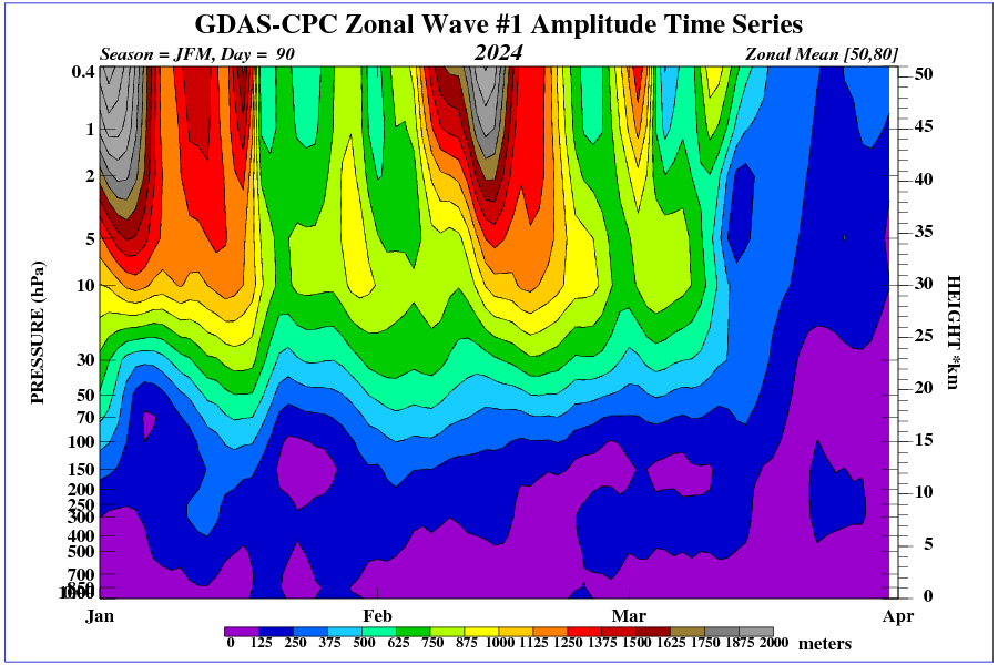
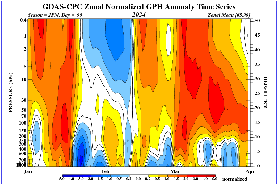
This may be related to the increase in GCR, whose cascades (secondary radiation) in high latitudes reach the very surface.
It should be remembered that the production of ozone as a result of UV radiation with a wavelength shorter than 242 nm on diatomic oxygen already occurs in the lower mesosphere, and the highest kinetic energy is reached by air molecules at the top of the stratosphere.
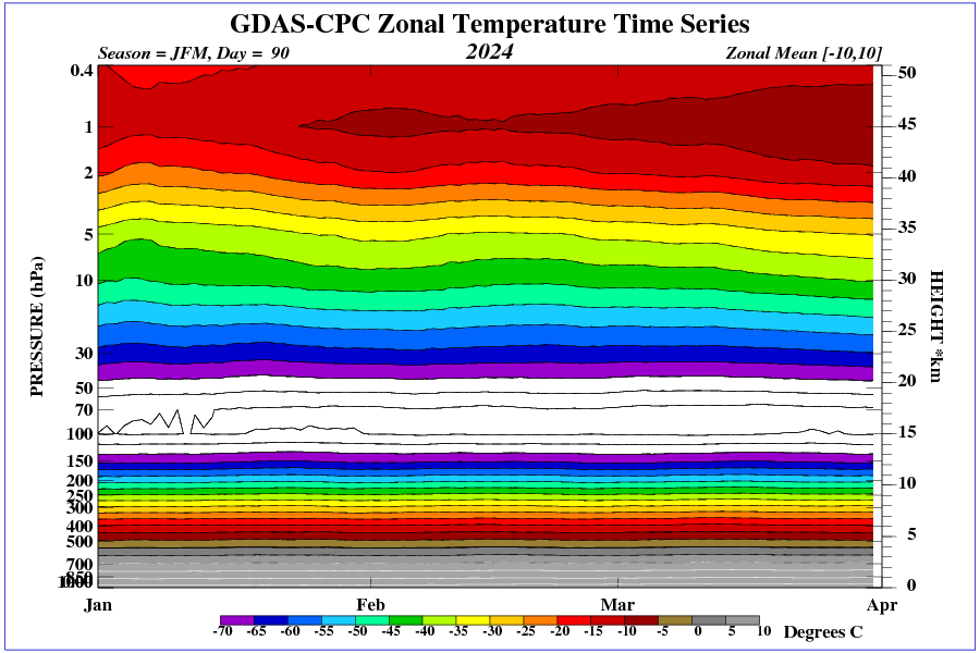
“This thermal energy transport is called the “meridional transport” of energy. When meridional transport is strong, Earth cools, and when it is weak Earth warms.”
I don’t get that. Increased poleward heat transport since 1995 caused a warmer AMO and Arctic, and Earth warmed. Did that increased poleward heat transport use up heat reserves from elsewhere? I don’t think so, low cloud cover has declined since 1995 allowing upper ocean heat content to rise.
Meridional transport can cause an increase in ocean surface temperature due to east wind interference along the equator and a decrease in subsurface temperature.


[QUOTE FROM ARTICLE]”In contrast to the tropics, the polar regions have the smallest greenhouse effect in the troposphere. This is especially true in the polar winter when the relative humidity is nearly zero due to the lack of sunlight and the low air temperature. This causes the air moving into the polar region to be warmer than the surface. The water under the polar ice is relatively warm (approximately -1.8°C) but it is insulated from the colder surface by ice. Thus, there is more radiant cooling to space from the polar air than from the surface because warmer bodies emit more radiation. In the dry polar regions, most radiation in the winter is from CO2, and adding more CO2 there means more radiation to space, which increases the rate of cooling, so we observe a reverse CO2-human-enhanced greenhouse effect during polar winters.”[END QUOTE]
This may explain why Antarctica is cooling while parts of the Arctic are warming. Most of the area south of the Antarctic Circle is land, which would be a “dry polar region”. Despite the fact that most of Antarctica is covered by ice, there is little precipitation or humidity there in winter, since the surrounding ocean is frozen over, which prevents evaporation.
Greenland is also a “dry polar region” in winter, except along its east coast where open water persists well into autumn due to the Gulf Stream, and storms can follow the sharp temperature gradient and dump snow on the land (similar to nor’easters along the east coast of the United States).
Outside of Greenland, most of the north polar region is ocean, nearly surrounded by land south of the Arctic Circle. In winter, the polar air emits more radiation, but in spring and summer, the land to the south loses its snow cover, and the ice melts around the southernmost parts of the Arctic Ocean. This open water promotes evaporation of water to form clouds, which limit the input of solar energy, and prevents temperatures from rising much above the freezing point.
If the major fear of “global warming” is rising sea levels due to melting of polar ice, this analysis would tend to dispel such fears. If the “dry polar regions” are getting colder, the ice sheets on Greenland and Antarctica will not melt. There may be some melting of sea ice (in humid polar regions), but since sea ice already displaces its weight of water, its melting will not affect sea level.