by Roy W. Spencer, Ph. D.
What follows is a response to Gavin Schmidt’s blog post at RealClimate.org entitled Spencer’s Shenanigans in which he takes issue with my claims in Global Warming: Observations vs. Climate Models. As I read through his criticism, he seems to be trying too hard to refute my claims while using weak (and even non-existent) evidence.
To summarize my claims regarding the science of global warming:
- Climate models relied upon to guide public policy have produced average surface global warming rates about 40% greater than observed over the last half-century (the period of most rapid warming)
- The discrepancy is much larger in the U.S. Corn Belt, the world-leader in corn production, and widely believed to be suffering the effects of climate change (despite virtually no observed warming there).
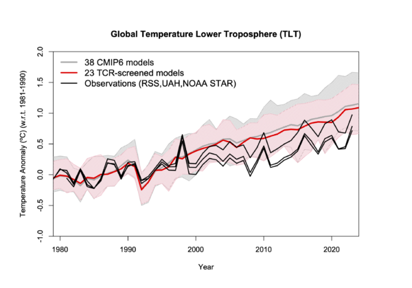
- In the deep-troposphere (where our weather occurs, and where global warming rates are predicted to be the largest), the discrepancy between models and observations is also large based upon multiple satellite, weather balloon, and multi-data source reanalysis datasets.
- The global energy imbalance involved in recent warming of the global deep oceans, whatever its cause, is smaller than the uncertainty in any of the natural energy flows in the climate system. This means a portion of recent warming could be natural and we would never know it.
- The observed warming of the deep ocean and land has led to observational estimates of climate sensitivity considerably lower (1.5 to 1.8 deg. C here, 1.5 to 2.2 deg. C, here) compared to the IPCC claims of a “high confidence” range of 2.5 to 4.0 deg. C.
- Climate models used to project future climate change appear to not even conserve energy despite the fact that global warming is, fundamentally, a conservation of energy issue.
In Gavin’s post, he makes the following criticisms, which I summarize below and which are followed by my responses. Note the numbered list follows my numbered claims, above.
1.1 Criticism: The climate model (and observation) base period (1991-2020) is incorrect for the graph shown (1st chart of 3 in my article). RESPONSE: this appears to be a typo, but the base period is irrelevant to the temperature trends, which is what the article is about.
1.2 Criticism: Gavin says the individual models, not the model-average should be shown. Also, not all the models are included in the IPCC estimate of how much future warming we will experience, the warmest models are excluded, which will reduce the discrepancy. RESPONSE: OK, so if I look at just those models which have diagnosed equilibrium climate sensitivities (ECS) in the IPCC’s “highly likely” range of 2 to 5 deg. C for a doubling of atmospheric CO2, the following chart shows that the observed warming trends are still near the bottom end of the model range:

And since a few people asked how the results change with the inclusion of the record-warm year in 2023, the following chart shows the results don’t change very much.

Now, it is true that leaving out the warmest models (AND the IPCC leaves out the coolest models) leads to a model average excess warming of 28% for the 1979-2022 trends (24% for the 1979-2023 trends), which is lower than the ~40% claimed in my article. But many people still use these most sensitive models to support fears of what “could” happen, despite the fact the observations support only those models near the lower end of the warming spectrum.
1.3 Criticism: Gavin shows his own comparison of models to observations (only GISS, but it’s very close to my 5-dataset average), and demonstrates that the observations are within the envelope of all models. RESPONSE: I never said the observations were “outside the envelope” of all the models (at least for global average temperatures, they are for the Corn Belt, below). My point is, they are near the lower end of the model spread of warming estimates.
1.4 Criticism: Gavin says that in his chart “there isn’t an extra adjustment to exaggerate the difference in trends” as there supposedly is in my chart. RESPONSE: I have no idea why Gavin thinks that trends are affected by how one vertically align two time series on a graph. They ARE NOT. For comparing trends, John Christy and I align different time series so that their linear trends intersect at the beginning of the graph. If one thinks about it, this is the most logical way to show the difference in trends in a graph, and I don’t know why everyone else doesn’t do this, too. Every “race” starts at the beginning. It seems Gavin doesn’t like it because it makes the models look bad, which is probably why the climate modelers don’t do it this way. They want to hide discrepancies, so the models look better.
2.1 Criticism: Gavin doesn’t like me “cherry picking” the U.S. Corn Belt (2nd chart of 3 in my article) where the warming over the last 50 years has been less than that produced by ALL climate models. RESPONSE: The U.S. Corn Belt is the largest corn-producing area in the world. (Soybean production is also very large). There has been long-standing concern that agriculture there will be harmed by increasing temperatures and decreased rainfall. For example, this publication claimed it’s already happening. But it’s not. Instead, since 1960 (when crop production numbers have been well documented), (or since 1973, or 1979…it doesn’t matter, Gavin), the warming has been almost non-existent, and rainfall has had a slight upward trend. So, why did I “cherry pick” the Corn Belt? Because it’s depended upon, globally, for grain production, and because there are claims it has suffered from “climate change”. It hasn’t.
3.1 Criticism: Gavin, again, objects to the comparison of global tropospheric temperature datasets to just the multi-model average (3rd of three charts in my article), rather than to the individual models. He then shows a similar chart, but with the model spread shown. RESPONSE: Take a look at his chart… the observations (satellites, radiosondes, and reanalysis datasets) are ALL near the bottom of the model spread. Gavin makes my point for me. AND… I would not trust his chart anyway, because the trend lines should be shown and the data plots vertically aligned so the trends intersect at the beginning. This is the most logical way to illustrate the trend differences between different time series.
4. Regarding my point that the global energy imbalance causing recent warming of the deep oceans could be partly (or even mostly) natural, Gavin has no response.
5. Regarding observational-based estimates of climate sensitivity being much lower than what the IPCC claims (based mostly on theory-based models), Gavin has no response.
6. Regarding my point that recent published evidence shows climate models don’t even conserve energy (which seems a necessity, since global warming is, fundamentally, an energy conservation issue), Gavin has no response.
Gavin concludes with this: “Spencer’s shenanigans are designed to mislead readers about the likely sources of any discrepancies and to imply that climate modelers are uninterested in such comparisons — and he is wrong on both counts.”
I will leave it to you to decide whether my article was trying to “mislead readers”. In fact, I believe that accusation would be better directed at Gavin’s criticisms and claims.
Addendum:
Gavin Schmidt has a long history of whining about Dr. Roy Spencer’s pointing out discrepancies between climate models and reality.
Steve McIntyre did a marvelous dissection of Schmidt’s knee-jerk criticisms in this 2016 post.
The above post inspired this cartoon from Josh.

And lets not forget Schmidt being unwilling to debate or even share a stage with Dr. Spencer.
Schmidt is a coward.
Well.. I guess he has all right to be that way.. but he also seems to be aww “slippery” .. when he knows his arguments won´t hold he chooses not to debate.. this way he was not defeated.. even everything he said was contradicted.. that is a political move.. and scientifically clearly unethical!
If anyone is pitching catastrophe, emergency, disaster, crisis- they don’t have a right to be a coward.
Gavin’s choice not to debate is based on experience. Many years ago, Gavin was part of a debate that teamed climate scientists and the like against skeptics. On the skeptics side were people like Michael Crichton. The skeptics won.
The full debate used to be on YouTube. Might still be,
Regards,
Bob
Update: I found the debate on YouTube. Here’s the link:
IQ2US Debate: Global Warming Is Not A Crisis (youtube.com)
Thx Bob. Extremely good debate. Gavin got his butt kicked. HIs contribution was nothing more than blanket statements with no evidence, sneering at opponents and showing that warmist scientists were little more than political activists.
Gavin Schmidt is a climate zealot. Roy Spencer is not. Who do you think is going to present a more accurate picture of climate trends?
Schmidt long ago gave up the right to be respected for his “scientific” opinions. He’s a charlatan, not a scientist.
This is the reason Gavin refuses to debate realists face to face, he would lose his. His pseudoscience blog consistently takes issues out of context to prove his nonexistent points.
The theme of his blog is that they are skeptical of climate skeptics. So, I asked there if it’s OK to be skeptical of those who are skeptical of climate skeptics. I was warned that any more comments like that and I’d be locked out. I never went back.
The challenge for scientists in publicly debating the contrarians is that the contrarians are not constrained by the truth, and it is almost impossible to counter well-constructed and orated lies to a credulous audience of non-specialists by using blunt and boring scientific facts. Audiences respond to compelling speakers, not compelling arguments.
By the same token, the reason the contrarians seldom try to engage in the scientific process and publish in peer reviewed journals is because it is impossible to slip well-constructed and written lies past an audience of specialists trained in the blunt and boring scientific facts.
Most of these constraints are removed in the boring old proceeds of Mann v Steyn. This is why prescient WUWT commenters on that are deflecting to whining about the “liberal” jury pool.
Gavin’s training is in applied mathematics. He is not a scientist. He has no training in science.
Gavin has hundreds of peer reviewed publications to his name and nearly 30,000 citations listed on Google Scholar. He is the director of the Goddard Institute for Space Studies. He is a professional scientist. It’s probably a good idea, in public, at least, to refrain from saying things you know are stupid. Just a bit of advice.
“It’s probably a good idea, in public, at least, to refrain from saying things you know are stupid”
Never stopped you !!
“ He is a professional scientist.”
He is NOT a scientist.. he is a mathematician, a data manipulator.
Please refrain from saying stupid things that you know are not constrained by the truth.
Tell us AlanJ, do you get a furry tongue from constantly licking Gavin’s….
….. boots !
Appeal to authority.
Just because other climate alarmists support him, is not proof that he is an authority.
Gavin’s training is in data manipulation.
GISS is the perfect place for him to push the AGW agenda.
“the contrarians is that the contrarians are not constrained by the truth”
This is arguing to the person and not to the facts.
You have not demonstrated *any* refutations of a*any* lies.
The really hilarious thing is that you think Schmidt is constrained by the truth.
We know you certainly are not.
The reason there is so much junk science in the climate journals is because they DO let very sloppily constructed lies pass through pal-review.. so long as it passes that AGW smell test.
blissfully naive , aren’t you Alan.
Mr. J: You have distilled this very nicely. We skeptics would gladly debate liars unconstrained by truth, because we find from experience that the truth will out. You won’t debate “contrarians” because YOU DON’T BELIEVE THE TRUTH WILL OUT! Tells us you don’t really believe your own posts. And you are dumb enough to say it outright! I won’t need to follow your comments any more. Thanks
Funny, how you actually believe that climate alarmists even know what the truth is, much less feel constrained by it.
Have Gavin Schmidt and Michael Mann ever been seen in the same room together at the same time?
Their ego’s wouldn’t fit.
If they did, the stench would be intolerable.
Their mothers were hamsters, and their fathers smelled of elderberries.
Sorry, had to do it.
Regards,
Bob
😂😂😂😂😂😂 and you did right.
Regards from another Bob
Do you suspect they are having an affair?
Not that there’s anything wrong with that.
Does anyone know a good lawyer?
He’s asking if they are the same person.
You just had to ruin a good joke
It was neither good nor a joke.
Thanks for the update.
Dr. Roy defends his writing and I shan’t try to add to that. However, …
Whenever I read such posts, I have the feeling that Richard Feynman was looking at the ClimateCult™ member when he said:
“ … It’s a kind of scientific integrity, a principle of scientific thought that corresponds to a kind of utter honesty — a kind of leaning over backwards. For example, if you’re doing an experiment, you should report everything that you think might make it invalid — not only what you think is right about it; other causes that could possibly explain your results; and things you thought of that you’ve eliminated by some other experiment, and how they worked—to make sure the other fellow can tell they have been eliminated.
AND:
“The first principle is that you must not fool yourself and you are the easiest person to fool.”
― Richard P. Feynman
When I read that I always think of Millican’s Oil Drop experiments.
In about 1969 when I was at college we had a young lecturer who had gained a PhD looking fir Quarks which I’d never heard of at the time. He said that Millican had rejected a lot of his results because they were way off the majority. He also said these results indicated a charge of a third of the proton.
Whether that was true or not I don’t know. But Millican got a pretty good value for the charge of a electron and Quarks are accepted as part of the Standard Model
The exact details of the discussion are a bit hazy after over 50 years
If you remember the ’60s, you weren’t there. 🙂
” a bit hazy “
Me also, but the name is Robert A. Millikan, with a k.
The Northern Hemisphere is warming and will continue to outpace the SH cooling from south to north. Hence global average temperature will continue to trend up and certain to accelerate as the shifting peak solar intensity moves northward. Zenith maximum solar intensity in the NH will increase by 80W/m^2 over the next 9,000 years it will exceed 1W/m^2/century for a good number of those years. So a lot of ocean surface warming to come.
Attached compares the change in land surface temperature from Jan 1980 to Jan 2022. It is quite clear that the places where most warming is occurring is near or below 0C. And it is not surprising why the snowfall in the NH is trending upward. Australian is mid summer and is cooler over the 42 years.
Using temperature anomalies and global averages hides what is actually occurring. It is deceptive and the stuff of scammers perpetuating the nonsense that CO2 somehow increases Earth;s energy uptake.
“And it is not surprising why the snowfall in the NH is trending upward”
That would be surprising to the Rutgers Snow Lab since it contradicts what they report
Perhaps Rick should have said “since 1990 snowfall in the NH is trending upward”- though from this graph it looks pretty flat since 1995.
Using 1990 as a start point, the low point in a 56 year dataset, would be EXTREME data mining.
Yet their winter snow chart is trending up since 1967.
And for Fall.
Only Spring has a downwards trend
Rutgers University Climate Lab :: Global Snow Lab
There are four seasons in each year. I presented a chart that includes a whole year … and you are just angry that I posted useful and relevant data
Oh dear.. dickie want snow all summer as well.
What a maroon !!
Just angry because I posted relevant data.
I did not make any comment about snow melting, which becomes a factor in the annual cover.
On average melt is still outpacing snowfall apart from Greenland. Greenland is still losing ice but only through accelerated calving as the warm oceans erodes any remaining ice shelves. Ice cover extent in Greenland is increasing and elevation is increasing.
What matters is the increasing autumn and winter snowfall. Numerous snowfall records were set again in 2023/24. That trend will continue for 9,000 years. My estimate is that snowfall will overtake snow melt within 200 years.
The Fall data is for the N Hemisphere the Winter data is not, be consistent.
bNasty2000 is inconsistent, nasty and deceptive about snow coverage. Three strikes.
little-dickie… data is from Rutgers.. Get over it, putz. !!
Typical liar
There is NH snow in Fall, Winter and Spring. You deliberately data mined the one of the three charts to support your deception. You are a loser.
So more snow in the Autumn and Winter ..
…. and less in Spring, when you actually want it gone so you can grow things.
You really hate losing, don’t you little child.
“The Northern Hemisphere is warming and will continue to outpace the SH cooling from south to north.”
Most of the Southern Hemisphere is not cooling.
Didn’t hadCRUT have something to do with Climategate?
The chart includes UAH too
You are even too dim to understand my implication.
Those “temperature trend” graphs are basically land area by latitude. There’s almost no difference until you get North of 60 N.
Correct. However your chart makes my point. The SH is cooling south to north and by far the most warming is occurring in the high northern latitudes.
The chart invalidates the CO2 warming nonsense because CO2 has been rising at 60S much the same as everywhere else. Any sustained cooling trend invalidates the “greenhouse gas” nonsense.
And your chart does not show the spatial and temporal detail that is important to understanding the changing climate.
The climate is much more complex than a single number can convey or even a single word like “warming”. To get a basic understanding, you need to at least look at regional and seasonal trends. Looking at those show significant trends that counter what climate botherers claim is happening.
“Hence global average temperature will continue to trend up and certain to accelerate…”
??? Should we panic?
Never panic. Climate change is gradual. The only change I have detected at 37S is faster growth of trees and that is more to do with CO2 than climate change. The summers may be moderating but would need a few more decades to cement a trend.
People living in the NH should expect to experience warmer summers and wetter or snowier winters depending on latitude with more snow north of 40N except along ocean coastlines. Growing seasons will continue to extend but summer water shortages may become more common.
There will need to be increased budgets for snow removal. Great, great grandchildren may observe the permafrost extending south by 2200. Glaciers will also be advancing by then.
I expect Northern Africa will be the most noticeable beneficiary of climate change. The Mediterranean is reaching the 30C temperature limit and this promotes the most powerful convective instability that leads to convective storms that will head south fuelled by the warm dry air over the land.
Maybe within 1,000 years, the oceans will be falling at a rate that threaten existing port infrastructure. Expect sea level to fall around 20m in the next 5,000 years. The rate of fall will be much faster than the present rise because we are close to the end of the present interglacial. The oceans will begin to fall not long after the ice starts to accumulate on the land again.
Freeman Dyson’s main criticism of the climate models was that they were not holistic. They didn’t consider the benefits of parts of the globe warming.
“I expect Northern Africa will be the most noticeable beneficiary of climate change”
This isn’t a negative no mater how much climate science wants us to believe.
(where did humanity originate?)
The warming of the NH has almost nothing to do with CO2
Water vapor is the 800-lb Gorilla; CO2 is a Pigmy
Here are the calculations
Water Vapor Compared With CO2 in the Atmosphere
https://www.windtaskforce.org/profiles/blogs/hunga-tonga-volcanic-eruption
.
CO2 in atmosphere was 423 molecules of CO2/million molecules of dry air at end 2023, or 423 ppm, but in densely populated, industrial areas, such as eastern China and eastern US, it was about 10% greater, whereas in rural and ocean areas, it was about 10% less.
https://svs.gsfc.nasa.gov/4990
.
Water vapor, worldwide basis: Water vapor is highly variable between locations, from 10 ppm in the coldest air, such as the Antarctic to 50,000 ppm (5%), such as in the hot, humid areas of the Tropics.
Water vapor in atmosphere, worldwide average, weight basis, is about 1.29 x 10¹⁶ kg, or 7.1667 x 10^14 moles
Atmosphere weight, dry, is about 5.148 x 10^18 kg, or 1.7752 x 10^17 moles
Water vapor percent, weight basis, is about 1.29 x 10^16 / 5.148 x 10^18 = 0.002506, or 0.2506%
Water vapor fraction, mole basis, is about 7.1667 x 10^14 / 1.7752 x 10^17 = 0.004037, or 0.4037%, or 4037 ppm
Water vapor molecules, worldwide average, are about 4037/423 = 9.54 times more prevalent than CO2 molecules
Water vapor in temperate zones, north and south of the equator, where most of the world’s population lives, is more prevalent, than the worldwide average of 4037 ppm.
Water vapor, in temperate zones, is about 9022 ppm, at 16 C and 50% humidity
Water vapor molecules, in temperate zones, are about 9022/423 = 21.33 times more prevalent than CO2 molecules
Water vapor in the Tropics, with high temperatures and high humidity, is much higher than elsewhere
Water vapor, in the Tropics, is about 29806 ppm, at 30 C and 70% humidity
Water vapor molecules, in the Tropics, are about 29806/423 = 70.46 times more prevalent than CO2 molecules
https://www.engineeringtoolbox.com/water-vapor-air-d_854.html
Allocating Available IR photons
.
We assume, for simplicity, H2O and CO2 molecules have equal global warming capacity.
About 22% of IR photons escape to space through an atmospheric window, per Image 11A, blue part. That leaves 78% to be allocated to H20 and CO2 molecules, as follows:
Worldwide basis: H2O molecules absorb 78 x 4037/(4037 + 423) = 70.6%, and CO2 molecules 7.4%; some sources state up to 8% of IR photons is absorbed by CO2
Temperate zone basis: H2O molecules absorb 78 x 9022/(9022 + 423) = 74.5% and CO2 molecules 3.5%
Tropics: H2O molecules absorb 78 x 29806/(29806 + 423) = 77%, and CO2 molecules 1%
It appears, CO2 has almost no global warming role to play in the Tropics, where huge quantities of water vapor is heated, that is distributed to the rest of the earth, by normal circulation processes.
If H2O molecules had greater global warming capacity than CO2 molecules, the CO2 role regarding global warming would be even less.
The reason water vapour is important is because it solidifies in the atmosphere. It makes up those white fluffy things we call cloud or sometimes the more ominous cumulonimbus variety.
There is a very simple relationship between cloud induced reduction in OLR and increased reflection over tropical warm pools. . The ratio of increased SWR to reduced OLR is 1.9. That is the cooling factor for clouds over 30C warm pools. The relationship for daily averages over tropical warm pools in the NH is:
SWR = 528 -1.9*OLR
So every W/m^2 reduction in OLR due to cloud formation over warm pools increases the reflected short wave by 1.9W/m^2. The daily average range in OLR over a warm pool is from 130W/m^2 to 255W/m^2.
It is a little different for warm pools in the SH because the sun is currently more intense in the SH.
Warm pools occur when the atmosphere and surface reaches thermal equilibrium within the constraints of the inevitabe cyclic instability. That occurs at 30C surface temperature in open oceans.
Cyclones can have much lower OLR radiating power than warm pools with OLR below 100W/m^2. But they also form the most reflective cloud. They are not in thermal equilibrium with the surface. They always result in net cooling but are fuelled by a source of warm, dry air to keep them spinning.
Clouds control the energy uptake and release. Their formation is related to the surface temperature. So solid water is important – radiative gasses not so much.
The impetus of what you describe is absorption of IR photons
Water vapor has wide absorption bands below 14.9 micrometers
Those photons are more energetic, so it is likely H20 molecules are much more potent than CO2 molecules, plus they are far more abundant than CO2 molecules.
For the life of me, I just do not understand how the IPCC and co-conspirators get away with their outrageous claims of evil regarding CO2
Heating the Entire Atmosphere by 0.3 C
.
This study shows, based on UAH satellite measurements started in 1979, lower-atmosphere temperatures have been increasing, step-by-step, and are pre-dominantly due to El Niños, and volcanic eruptions, such as Hunga Tonga, and their after effects.
.
Calculation: Image 7 shows, an increase of the lower-atmosphere temperature of about 0.3 C in late 2023.
This was due to:
1) A strong El Niño peaking in late 2023, which increased water vapor, over a period of time (months) in the
lower-atmosphere
2) The after-effects of the Hunga Tonga eruption, which temporarily increased water vapor by 10 to 15%, in a very short time, in the lower-atmosphere
Q = mass x Cp x delta T = (5.148 x 10^18 kg) x (1012 J / kg.C) x (0.3 C) = 1.563 x 10^21 = 1563 exajoules
Almost all of that energy was IR photons, absorbed by water vapor molecules
Human primary energy production for all uses in 2022 was estimated at 604 exajoules
.
Night-time Energy Loss Regained the Next Day
.
The lower-atmosphere temperature usually has a 15 C up and down with day and night, which is a lot of energy lost by the lower-atmosphere to space at night, to be regained the next day, when it faces the sun again.
The regain energy is about 15/0.3 x 1563 = 78150 exajoules during a 12-h daytime, which compares with human primary energy production of 604/(365 x 2) = 0.83 exajoules per 12-h
Human 12-h energy use is totally insignificant compared to solar 12-h energy input
The Earth would be a cold place without that solar energy.
That huge energy gain would not be possible without:
1) significant IR photon absorption by water vapor in high humidity/high temperature areas, such as the Tropics, and
2) significant mass transfer of energy within the lower-atmosphere to distribute that energy
Thanks, Roy, for, first, preparing something that tweaked the clowns at RealClimate again, and then, second, for preparing this rebuttal. This exchange brings back fond memories of battles between RealClimate and WUWT from years ago.
And thanks, WUWT, for cross posting this here.
Regards,
Bob
I also posted the links and a short excerpt in a comment at CFACT…and on a couple of Conservative blogs….spread the word is my philosophy.
https://www.cfact.org/2024/01/31/the-defense-get-its-turn-in-the-climate-trial-of-mann-v-steyn/#disqus_thread
“battles between RealClimate and WUWT from years ago”
hmmm… I missed that- should happen again!
RealCimate has decided that it will only communicate with people who already agree with it.
I seem to recall- last time I looked- a few years ago- they have some web pages or maybe a booklet- about how to talk to “your retarded dumb ass uncle the climate denier”.
Wow, I never viewed that show before.
I started asking NS why he h@Alfred Ledner poor people multiple times and came up with the ideas that envirowacos h@te poor people and love their crony capitalists on my own.
I know I am not as smart as Roy.
After hearing Gavin, a Mann clone even to the bald head and arrogance, I know I AM smarter than those two.
But of course I also don’t h@te poor people.
Arrogance abundant, common sense nowhere to be found.
And dickie-bot is trying to outdo that. !
Even if Schmidt were right it would be hard to watch him.
oh he doesnt do television.. except when he does.. lol.. what an eel!
As I understand it, the alarmists camp caution their bought people not to debate a sage free thinking skeptic because the skeptic would wipe the floor with them using facts, data, historical record, 1979+ sat info, etc. Facts and data in science always trump (intended) the emotional nonsense of alarmists – Schmidt on Stossel reminds me of biden in a basement.
Alex Epstein mopped the floor with Bill McKibben about 7 years ago in a debate which is still on YouTube.
In 2016 he his estimate of climate sensitivity was 2.5C – 3C.
https://www.youtube.com/watch?v=z9lun__zZTs
2C , 2.5C, 3C, it all sounds like a dispute over how many angels can dance on the head of a pin.
Gavin Schmidt on the NASA website:
“.. a few degrees might not seem like much, it’s a big deal for the planet. The difference between forests beyond the Arctic Circle or glaciers extending down to New York City is only a range of about 8 K (about 14 degrees Fahrenheit) in the global average, while it changes sea level by 150 meters (more than 400 feet)!”
Changes in grounded ice and sea level of that magnitude take tens of hundreds of years.
Very low resolution estimates of the average temperature reached during the last interglacial are around 4C above the current average.
There was nothing predetermined or ‘heaven-sent’ about the global temperature and CO2 levels in 1950.
As ever adaption is the only sane response to whatever the future climate brings.
“the average temperature reached during the last interglacial are around 4C above the current average.”
Correction
The average temperature reached during the first 2/3 of THIS interglacial was around 3-4C above the current average.
Tree lines, trees under glaciers, sea levels, permafrost peat beds, sea ice extent, animal remains…. etc etc… confirm this.
“The average temperature reached during the first 2/3 of THIS interglacial was around 3-4C above the current average.”
Yu have no data to back that false claim. About 1.3 of the current interglacial is believed to have been warmer than2023, but the evidence is not very strong (for the ENTIRE period from 5000 to 9000 years ago), and not based on instruments.
Plenty of data has been posted MANY TIMES.
It is just that YOU remain deliberately ignorant.,.
Stop DENYING science.
STOP DENYING the Holocene optimum.
It makes you look like a MANIC AGW CULTIST.
Even the MWP was warmer than now
Or are you also a MWP-denying-nutter ??
Only the LIA was colder.
You are overdosing on stupid pills … again.
The Holocene Climate Optimum (HOC) reconstructions, when averaged to create a fake global average, only suggest that some periods of the HOC were warmer than 2023. not a majority of the HCO.
You just invent factoids as you go along and toss insults at anyone who refutes your OBVIOUSLY false claims. You are a loser.
Most likely less than 20% of the past 12000 years were warmer than 2023, NOT 2/3. And that is using a comparison of averaged local reconstructions — a fake global average — with instrument data, which is a poor comparison.
The data has been presented, many times. Against that we have RG whining that it is fake.
BTW, I love how the guy who whines about insults, is so quick to use them when he has no arguments.
You haven’t refuted ANYTHING, just manic DENIAL of science and data.
It is shown by data that in every regions of the world, the Holocene was 3 or significant more, degrees warmer than now and remained warmer right through the RWP and the MWP, up until the cooling into the LIA
You ARE a Holocene-denying nutter
…. and a MWP-denying nutter
Outing yourself as a true died-in-the-wool AGW cultist nutter..
It doesn’t matter how much the CAGW advocates whine and cry they won’t be able to control what happens. The earth will do what the earth will do. The only real answer is to adapt and killing off half the human population from lack of energy is *not* adapting, it is submitting. Most of the species that ae extinct today are so because they couldn’t or wouldn’t adapt – which includes the political left today.
Is Gavin Schmidt like a broken clock, correct a couple of times a day and wrong all the rest of the time?
Gavin Schmidt Explains Why NOAA Data Tampering Is ILLEGITIMATE
In 2010, NASA’s Gavin Schmidt explained why NOAA’s FAKE DATA wrecks the US temperature record.
https://realclimatescience.com/2017/01/gavin-schmidt-explains-why-noaa-data-tampering-is-illegitimate/
From that link:
Just a handful of stations for over 3 million square miles? That’s sufficient for SCIENTIFIC conclusions? Sufficient to drastically change our civilization?
Scientists who create or study models are allergic to the truth about models
There are no climate models
There are just computer games called models
A real climate model would have to include knowledge about perhaps 10 manmade and natural causes of climate change. No such knowledge exists.
Even if such knowledge existed, there is no evidence that the future average temperature could be predicted in 100 years, 50 years, or even in 1 year.
Computer games predict whatever they are programmed to predict.
They programmed to predict whatever their owners want predicted (whatever predictions will get accepted by a consensus).
Climate computer games have no value except as climate propaganda. I call them Climate Confuser Games
Predictions of a coming global warming crisis do not need climate models. They also do not need, or have, any data. They are just climate astrology, wrong since the 1979 Charney Report (+1.5 to +4.5)
Climate change is data free, wrong since 1979, predictions of global warming doom. These predictions may be stated by scientists but they are not science. Science requires data. There are no data for CAGW. Because CAGW is just an imaginary climate.
To be more specific, climate predictions have been wrong since 1896:
In 1896, a paper by Swedish scientist Svante Arrhenius first predicted that doubling of atmospheric carbon dioxide levels could substantially alter the surface temperature through the greenhouse effect.
Being from cold Sweden, with a climate like Minnesota, he didn’t see global warming as bad news.
Not much has changed since 1896, except the IPCC’s scary CO2 prediction is less scary than the world heard in 1896, and scientists now say climate change will kill your dog.
Greene….
Also Greene…
Are you talking about predictions now or do you have the data ”science requires”?
For you… ” in science, the term data is used to describe a gathered body of facts.”
….. ” Fact ..a thing that is known or proved to be true”.
I’ll wait……..
Fact:
You are a nasty man with nothing of value to say
Data:
Your comment
Lab measurements in the 1800s created the first estimate of temperature effects of CO2 x 2 and CO2 / 2
Those experiments isolating CO2 in a lab created data used for a conclusion about CO2 in the atmosphere.
It is a fact that data were collected in the 1800s and a scientific conclusion was derived from those data.
Have someone read my comments to you and explain them.
Fact,: little-dickie is a slimy, arrogant, self-opinionated, anti-science, moronic AGW nutter…
… with ZERO CREDIBILITY on anything to do with CO2 affecting climate. !
CO2 warming is nothing but “conjecture”… certainly that is all Arrhenius had.
The Earth is NOT a glass laboratory jar.
All he showed was that CO2 is a radiatively active gas..
That is all you can possibly prove using glass jars.
You still have NO EVIDENCE OF ATMOSPHERIC WARMING BY CO2.
Your comments contain absolutely NOTHING pertaining to science, just gabble. !.
Get your low-IQ 10-year-old “friend” to explain that to you.
I have much evidence that you are an angry CO2 Does Nothing Nutter with a desire to post all insults and no science. You are the Don Rickles of the website, but not funny, and the Forrest Gump of climate science, which is funny.
You act like a 12 year old who claims to know more than almost 100% of climate scientists who have lived on this planet in the past century.
It takes a special talent to think yourself as being so smart, yet sounding so dumb with your comments. You do disguise your alleged intelligence very well, by pretending to be a Floyd. R. Turbo of climate.
Classic Floyd R. Turbo | Carson Tonight Show (youtube.com)
Yet you still haven’t produced a single bit of evidence for warming by atmospheric CO2.
Your puny little low-IQ rant is NOT evidence of anything except the fact that you are mentally deranged.
I’ve been saying for years that the climate sensitivity for CO2 is around 0.2 to 0.3C. Given that we are only about half way through the current doubling, and given that the oceans have a huge thermal lag, the amount of warming created by CO2 is less than 0.1C, possibly in the 0.05 range.
It’s hardly surprising that such a small amount of warming is undetectable in the highly variable climate signal. (Assuming we could measure temperatures down to the 0.05C level)
The fact that we can’t detect the signal is not evidence that CO2 has no impact.
Hold a second Mr Twonk. Tell us EXACTLY…What do ”scientists know?”
The ”data” you cite was used to arrive at HYPOTHESIS. You cannot reach a ”conclusion” without testing the hypothesis with experiment. Tell me Greene, were did you first become confused?
Note the idiotic anti-science claim to a faked consensus… again… !!!
Seems be the only “evidence” he has. 🙂
The experiment in the lab- interesting tidbit of knowledge. Concluding that the atmosphere behaves the same way is absurd. I see that Arrhenius used the weasel word “could”. He didn’t say it was a fact- a proven fact- only that it COULD happen.
Science does not prove or disprove anything.
Your comment does prove you are a CO2 Does Nothing Nutter science denier.
You certainly haven’t got any science to prove anything .
That is because your understanding of science is extremely poor and limited.
You keep proving that.
Oh and your little rants are getting more and more mentally deranged.
Great for the popcorn trade !! 🙂
The further behind he falls, the nastier RG gets.
It is like watching an ADHD 5-year-old having a tantrum because his mother wouldn’t let him have a lolly !
Funny, in an embarrassing sort of way.
Conclusion? Lol. It has never got past the hypothesis stage. Your argument is worthless. You must separate human co2 from natural variability otherwise you are talking garbage. Maybe if some one else explained it to you…?
Good luck. I’ll wait….
It is also a fact that my cat eats tuna. There are all kinds of irrelevant facts around just like yours.
Let me fix your quote.. It is a fact that data were collected in the 1800s and a scientific
conclusionhypothesis was derived from those data.“I’ll wait……..”
You will never get anything remotely resembling scientific proof of CO2 warming from little-dickie.
He doesn’t have any.
All you will get is his normal low-IQ rants.
bNasty is Dand Dumber combined
Thanks for proving you can’t produce any evidence. AGAIN !!
I wonder why he is so angry, but he was angry for my deleting a SINGLE post at a science blog I administrate a few weeks ago.
It may be true that there is SOME warming from CO2 but it’s not yet a proven fact. It COULD be true, like a lot of things that COULD be true but are not. And if it is true, it’s most likely minor, not worth drastically changing our civilization in a panic mode.
“A real climate model”
A real climate model would be holistic, taking in all effects of temperature change around the globe. This was Freeman Dyson’s main criticism of the “temperature” models. They are not holistic. They do not include any impact from increased food harvests, fewer cold deaths, less catastrophic weather, etc. The entire CAGW crowd considers a warming globe to be a catastrophe when it likely isn’t. If *everyplace* on earth warmed 4F food crops would prosper, both from longer growing seasons as well as increased CO2. Energy demand would go down leading to a tepering off of CO2 production. And on and on and on ……
The climate models are a piss poor metric for ANYTHING. It is enthalpy that is important and the climate models don’t even look at enthalpy although the data has been available for 40 years or more.
We will be forever indebted to Richard Feynman. Any new theory is just a guess. How do we know if it is valid or not?
“If it disagrees with experiment, it’s wrong. In that simple statement is the key to science. It doesn’t make any difference how beautiful your guess is, it doesn’t matter how smart you are who made the guess, or what his name is … If it disagrees with experiment, it’s wrong.”
The premise of ECS with a huge range- is barely a premise and barely science. Science is precise, like the mass of a proton: 1.67262192 × 10⁻²⁷ kilograms. And I bet there isn’t much debate over that FACT. When they can prove what the ECS is to that many decimal places, I think we can then say we have some science.
0.00000000
Dear Dr Spencer,
Has anybody taken a deep-dive into any corn belt temperature datasets. I don’t mean have they read the metadata (which is often faulty), or tossed the data against the wall to see what sticks using Excel, I mean, have they actually sat down with datasets and metadata and teased them for all their hidden signals? For example, the site changes that happened but were not reported, or those that were reported but which made no difference. On our side of the climate debate, a consistent, objective methodology for assessing individual station data is missing in action.
I make the point with respect, that trend analysis is not all about pictures and surveys and classifications (which are all useful), it is 90% about the data and whether they are homogeneous (not affected by non-climate factors). Averaging across faulty data derives a faulty average no matter how it is done.
I continually hear the claim that “we know temperature has increased”, but who are those that say it has? Which data did they use; how did they arrive at the conclusion? As far as I can work-out those that make the loudest noise have no experience in taking weather observations, none have started with a clean-slate of data, they universally use off-the-shelf datasets, and most draw conclusions that support causes. Bjørn Lomborg is a typical example, but there are many others.
An expert is someone who can defend their case, but for most, they depend on others or they just have not done the work.
Australian temperature data contributes to global datasets. However, physically-based, objective, replicable BomWatch protocols shows individual weather station datasets are dominated by site-change and rainfall effects, and that no trend or change is attributable to the climate.
In making claims about warming of surface temperatures, we MUST adopt transparent, objective and defendable protocols, and avoid making ambient claims based on climate hearsay or off-the-shelf datasets that may be biased.
Yours sincerely,
Dr Bill Johnston
http://www.bomwatch.com
Woops,
Dr Bill Johnston
http://www.bomwatch.com.au
I live in Kansas. Lots of corn here. Here are a graphs of long term temperatures in Topeka, Kansas. Most months show similar trends.
I know you will see that there are missing years in the middle. Yet, the trends match up on either side without any manipulation. Any growth would have shown disjointed trends. FYI, the station used is at an old airbase that was closed and not rejuvenated into an active airport for many years resulting in the missing data.
RSS?
Nope. USN00013920, Topeka Forbes
I processed the data using the procedure in NIST TN 1900. The anomaly SD was calculated by using the variance of the single month and the variance of the baseline. The anomaly mean was done by subtracting the mean of the month from the mean of the baseline. The SD of the anomaly was calculated by adding the variances using RSS and doing a square root, i.e., √(SD_month² + SD_base²).
Whoops! I just looked the graph and see what you were asking about. RSS stands for Root·Sum·Square. That is, the square root of the sum of the squared standard deviations. It is done when adding uncertainties when they are stated as a ± interval.
Dear Jim,
Where did you get “the variance of the single month from? Is it the variance calculated from daily values? Also, monthly anomalies are usually calculated by subtracting the baseline mean from respective months data (not the other way around as you seem to indicate). RSS conventionally refers to the Residual Sums of Squares (search for RSS statistics – I get About 822,000,000 results (0.34 seconds)).
As far as I can work out the ‘Root Sum Square method’ has to do with tolerance analysis for mechanical engineering applications (which I am not familiar with) [see: https://www.fiveflute.com/guide/introduction-to-root-sum-squared-rss-tolerance-analysis/%5D. I have never seen the method used in the context of processing surface temperature data, and I don’t see how it is relevant to spot data.
It may also matter that within month daily temperatures may not be normally distributed about the mean for the month.
Yours sincerely,
Dr Bill Johnston
“As far as I can work out the ‘Root Sum Square method’ has to do with tolerance analysis for mechanical engineering applications “
Then you’ve never studied metrology or read the GUM (JCGM 100-2008). That seems to be a common problem in climate science.
In the GUM, Equation 10 is the equation for propagating measurement uncertainty. It is the root-sum-square process.
” I have never seen the method used in the context of processing surface temperature data, and I don’t see how it is relevant to spot data.”
Of course you haven’t seem it used *anywhere* in climate science. That’s because the common assumption in climate science is that all measurement uncertainty is random, Gaussian, and cancels. Therefore the stated value of the temperature from a station is 100% accurate, i.e. no measurement uncertainty.
It’s how climate science can find differences in temperature down to the milliKelvin with the measurement devices have measurement uncertainty in the tenths digit at least and likely in the units digit. It’s why “trends” established by climate science are so unbelievable.
It’s why a Tmax and Tmin temperature reading should be given as 20C +/- 0.5C as an example. If both temperatures are from the same station with the same +/- 0.5C measurement uncertainty then the median should have, as the worst case, a direct addition of 0.05C + 0.05C or 1C. If it is assumed that some random cancellation occurs then you add the measurement uncertainties by root-sum-square and get a total measurement uncertainty of +/- 0.7C.
If you measurement uncertainty is +/- 0.7C then there is no way to find a difference in milliKelvin, the difference is subsumed by the measurement uncertainty, i.e. the difference becomes part of the GREAT UNKNOWN.
Averaging doesn’t reduce the measurement uncertainty of the mean nor does the measurement uncertainty become the SEM.
I think you know all this. I’m not sure why you are playing ignorant about the use of root-sum-square in metrology.
Dear Tim,
You have ignored the three issues I raised, namely:
Where did you get “the variance of the single month from? Is it the variance calculated from daily values? Also, monthly anomalies are usually calculated by subtracting the baseline mean from respective months data (not the other way around as you seem to indicate). RSS conventionally refers to the Residual Sums of Squares (search for RSS statistics – I get About 822,000,000 results (0.34 seconds)).
So where does the variance you drum-on about come from? How is it calculated? Give an example using real data.
And why do you deduct respective months data from the base and not the base from respective months data? [Differences will be the same but their signs will be opposite.]
In statistical parlance, RSS is the residual sum of squares. You are actually referring to ‘Root Sum Square method’, which is a statistical tolerance analysis method. Can you explain why you use such a method on temperature data?
You say: “The SD of the anomaly was calculated by adding the variances using RSS and doing a square root, i.e., √(SD_month² + SD_base²).”
As there is no divisor, the formula [√(SD_month² + SD_base²)] may not be correct (see for example: https://www.statisticshowto.com/pooled-standard-deviation/). Also see: https://cfmetrologie.edpsciences.org/articles/metrology/pdf/2013/01/metrology_metr2013_03003.pdf
I don’t see how this analysis approach applies to temperature measurement over time and the overarching issue of determining trend.
Yours sincerely,
Dr Bill Johnston
http://www.bomwatch.com.au
Look at the image. It is a piece of a spreadsheet for 2022 that shows the calculations. There is a sheet for each year.
That is exactly correct. A respective month is summed over all the years and a baseline mean and uncertainty is calculated. The uncertainty is calculated using the method in NIST TN 1900.
I searched for “RSS uncertainty” and got 13,400000 results.
https://pathologyuncertainty.com/2018/02/21/root-mean-square-rms-v-root-sum-of-squares-rss-in-uncertainty-analysis/
https://www.me.psu.edu/cimbala/me345web_Fall_2014/Lectures/Exper_Uncertainty_Analysis.pdf
You haven’t seen it because metrology methods have never been properly identified and used in climate science as it is in every other applied science such as physics, chemistry, and engineering.
The statisticians being used in climate science have no background in making measurements and all think that uncertainty goes down through dividing by √n. Nothing could be further from the truth.
I am not surprised you have never seen it used. Statisticians always assume the measurements are 100% accurate, occur in in a Gaussian distribution, and the Standard Error properly defined the sampling uncertainty of the calculations.
I have encountered people both here and on X that have no idea that at least in the U.S. NOAA defines the measurement uncertainty for ASOS mechanized stations as ±1.8°F. That is for each and every station and each and every measurement.
The values I am showing as SD or RSS are for the anomalies of monthly temps.
A monthly anomaly is calculated by subtracting two random variables (monthly – baseline) that have a mean and uncertainty. When adding or subtracting random variables their variances ADD. I have added them using RSS to calculate the value for each month and plotted their values on the graph.
As you can see, values inside the uncertainty interval are nothing more than a guess even if high powered computers calculate them.
It is one reason that temperature data samples twice daily is really unfit for the purpose it is being used for.
What are you talking about?
NIST TN 1900 Section E2, Surface temperature (p 29) bears no relationship to the stuff you have been going-on about (https://nvlpubs.nist.gov/nistpubs/TechnicalNotes/NIST.TN.1900.pdf). As for the GUM, it is more like a word salad held together with complex algebra (see attached) than a how-to-do handbook, as we have discussed before.
In fact NIST assumes that E1, …, Em are modeled independent random variables with the same Gaussian distribution with mean 0 and standard deviation, which is the direct opposite of your thoughts on the matter.
Whether the mean of the 22 datapoints truly represents the long-term monthly mean could easily be settled with a 1-sided t-test without the need for all the remaining (inconclusive) verbage. There is no mention of anomalies, and no mention of the ‘Root Sum Square method’. I have no idea from reading it, why NIST published such a document.
Cheers,
Bill Johnston
Look at the equation again. It is the sum of squares is it not. Uncertainties are expressed as standard deviations so one must take the square of the uncertainty before adding. Once added, the square root of the sum is taken to convert the sum back to standard deviation. Consequently, Root•Sum•Square! Think of what RMS stands for
Dear Tim,
I have spent the best part of an afternoon doing what I thought you would have done being the ‘expert’ commentator. I chased through numerous references, re-read some of the GUM, and downloaded and read relevant parts of NIST Technical Note 1900 and other reports that I rarely have any interest in.
I think I have now worked out the basis of our disagreement. I also searched https://www.itl.nist.gov/div898/handbook/index.htm using the search term root sum square. You could do that too.
The issues that are the focus of your concerns relate to the instrument (the thermometer, PRT-probe or whatever), whereas the focus of everyone else (including myself) is on the variable being measured (the temperature of the air within a Stevenson screen or its equivalent). You seem to have inverted that reasoning both statistically and in practice.
As described here (https://www.itl.nist.gov/div898/handbook/mpc/section5/mpc52.htm) and on following pages “The procedures in this chapter are intended for test laboratories, calibration laboratories, and scientific laboratories that report results of measurements from ongoing or well-documented processes”. The processes do not extend to the use of laboratory-calibrated instruments to derive measurements in the environment. Testing in a laboratory using NIST protocols provides assurance that field observations have a valid reference.
Positing that variation in environmental variables reflect instrument uncertainty is an inversion of logic that is simply wrong. Instrument or calibration uncertainty determined in a laboratory is (a usually small) +/- constant (Type A). However, in practice is it ½ the interval range, which in Australia is 0.5 degC (Type B). As Type B +/- (eyeball) error dominates in the field, and Type A +/- error provided on the calibration certificate (water-bath or other benchmark) is much smaller, calibration error is safely disregarded. (This does not mean the instrument is bad, it means the laboratory calibration process is more precise.) Although in storage they may deteriorate, well cared-for, calibrated instruments have a lifespan of a decade or more. It should also be a giveaway to your reasoning that instrument uncertainity is alwsys expressed as +/- each side of the mean (i.e., uncertainity is Gaussian or normal in its distribution, and therefore cancels out).
As explained in various publications including the NIST reference above, the root sum square only applies to calibration of the instrument used to take measurements. It does not apply to comparing values measured by an instrument in the field, where variation is a product of the environment, not the instrument. Furthermore, while you are welcome to your view, expressed as +/- each side of the mean implies that uncertainty is Gaussian or normal in its distribution, and therefore cancels out. A single observation can be expressed as Y +/- instrument uncertainty.
Standard error of a mean also has a defined statistical meaning, as does Tmax+Tmin/2, which is average-T, and not the median as you are prone to stating.
Yours sincerely,
Dr Bill Johnston
http://www.bomwatch.com.au
Did you read this link?
https://users.physics.unc.edu/~deardorf/uncertainty/UNCguide.html
I am not sure what you read, but do a little more studying. TN 1900 is not about instrument calibration. It is about analyzing field data. There are numerous examples about making and how to determine uncertainty.
The whole reason for trying to educate folks to the fact that LIG temperatures recorded as integers simply can not be averaged and obtain temperatures in the one-thousandths place with uncertainty in the same precision. No applied science allows this to occur. If climate science wishes to advance to the point it can be claimed to be an applied science, then the analysis of measurements must meet accepted procedures and rules.
Here is the problem with claiming that an SEM is a measure of uncertainty. I have a RIGOL oscilloscope that interfaces with my computer. It has a resolution of 0.001 with an uncertainty of 0.001. (I didn’t dig out the manual but these are close). I can set it to collect a reading every tenth of a second until I get one million readings. I can have an average of 0.501 volts and a Standard Deviation of 0.071. The SEM will be (0.071 / √1,000,000 = 7.1×10⁻⁸). Which of the following best informs people of the measurement uncertainty of your measurements?
0.50 ±0.00000007
or
0.50 ±0.07
Do you think the top value tells people the range of values they should obtain when measuring similar things?
Does not have anything to do with what we are discussion.
I don’t need an oscilloscope – R can calculate 1-million temperature readings with a mean of 27.5 degC and a stated distribution statistic within a stated range and do exactly the same thing, then calculate an SEM for that mean and back-calculate from the input parameters an SEM and they will be the same out to several decimal places.
> library(MASS)
> #empirical=T forces mean and sd to be exact
>
> x <- mvrnorm(n=1000000, mu=27.5, Sigma=10^2, empirical=T)
> mean(x)
[1] 27.5
> sd(x)
[1] 10
> Se <- (sd(x)/sqrt(length((x))))
> Se
[1] 0.01
>
> #empirical=F does not impose this constraint
>
> x <- mvrnorm(n=1000000, mu=27.5, Sigma=10^2, empirical=F)
> mean(x)
[1] 27.51956
> sd(x)
[1] 9.994417
> Se <- (sd(x)/sqrt(length((x))))
> Se
[1] 0.009994417
>
So what?
Aside from a waste of time, what does it mean?
I’m getting bored with this.
Cheers,
Bill
Are you joking? Temperatures are MEASUREMENTS! They should be treated as such and follow international standards for analyzing measurement data.
The GUM is only one document. There is also JCGM 200:2012 and numerous ISO documents. NIST has numerous documents. Canada and Europe also have documents covering measurement uncertainty. From your comments I get the impression you are not up to date on how measurements should be evaluated.
TN 1900 is an EXAMPLE showing a method of finding a portion of the measurement uncertainty in a monthly Tmax average. Of course they make some assumptions that allow emphasis on the main point. The make the assumptions very plain
Do you think climate scientists averaging daily temperatures don’t make similar assumptions? Do the calculations for baselines ever have a variance calculated?. Are they Gaussian? Is uncertainty ever propagated when a global average is calculated? How is an uncertainty of 0.05 ever arrived at when ASOS stations start with an uncertainty of ±1.8°F?
Dear Jim,
Maybe you should read https://nvlpubs.nist.gov/nistpubs/TechnicalNotes/NIST.TN.1900.pdf again.
I grabbed the Tmax data and pasted it to a stats pack.
Five statistical tests, including a Monte-carlo simulation, and a Q-Q plot showed data were normally distributed.
The mean was 25.6 with 95% distribution-free bootstrapped CIs of between 23.95 and 27.27 degC. The SEM was 0.9 (0.65 to 1.06 bootstrapped 95% CI).
Therefore for a value to be different it would have to exceed +/- (t(DF 21, 0.05) = 1.72*SEM = +/- 1.55 degC, which agrees pretty closely with -1.65 & + 1.67 degC calculated from the bootstrap.
Their uncertainty range (23.8 ◦C, 27.4 ◦C = (+/- 0.8)) seems wide. However, this is because they used the 97.5th percentile of Student’s t distribution with 21 degrees of freedom, not the 95th (P = 0.05) percentile. You could repeat the above calculation using t(DF 21,0.025 = 2.08 * SEM (=1.87) and arrive at the same interval, plus some rounding errors.
Aside from nit-picking What else is there to know?
All the best,
Bill Johnston
Data:
Data:
Day MaxTemp
1 18.75
2 28.25
3 25.75
4 28
7 28.5
8 20.75
9 21
10 22.75
11 18.5
14 27.25
15 20.75
16 26.5
17 28
18 23.25
21 28
22 21.75
23 26
24 26.5
25 28
29 33.25
30 32
31 29.5
I think that should be ±1.8 and no ±0.8
The correct table value to use is the two-tailed. See this link for an explanation. Look at the graphs and you’ll see why right away.
https://statisticsbyjim.com/hypothesis-testing/one-tailed-two-tailed-hypothesis-tests/
If someone uses this method, I will not protest a lot. Whether one quotes the SD of ±4.1°C or the expanded standard uncertainty of the mean of ±1.8°C in this situation they are both pretty large.
The big point is the values currently being portrayed for values and uncertainty.
The other issue is that other uncertainties were disregarded in an effort to make an example. Things like measurement uncertainty and systematic influences.
You are joking!
There is no such thing as a 2-tailed t-table!
What I said was:
Therefore for a value to be different it would have to exceed +/- (t(DF 21, 0.05) = 1.72*SEM = +/- 1.55 degC, which agrees pretty closely with -1.65 & + 1.67 degC calculated from the bootstrap.
Here is the really complicated math:
For a value to be different it would have to exceed +/- (t(DF 21, 0.05) = 1.72*SEM = +/- 1.55 degC, which agrees pretty closely with -1.65 & + 1.67 degC calculated from the bootstrap.
I.e.:
25.6 – 1.55 = 24.05 (b/s = 23.95) (lower)
25.6 + 1.55 = 27.05 (b/s = 27.27) (upper)
I also said they chose the 97.5th percentile of Student’s t distribution with 21 degrees of freedom (P = 0.025), not the 95th (P = 0.05) percentile. This corresponds with their uncertainty range of 23.8◦C to 27.4 ◦C [i.e., a confidence interval of +/- 0.8)].
I then invited you to “repeat the above calculation using t(DF 21,0.025 = 2.08 * SEM (=1.87) and arrive at the same interval, plus some rounding errors”.
In continuing to mix-up the difference between instrument uncertainty and T-values measured in the environment, your misuse of terms including SEM, and poor analogies, I think you are building a head-of-steam over nothing!
Cheers,
Bill
I’m sorry but there are. Look at the image.
There is no mix-up.
From the GUM
G.3.2 If z is a normally distributed random variable with expectation μ z and standard deviation σ, and z is the arithmetic mean of n independent observations zk of z with s(z ) the experimental standard deviation of z [see Equations (3) and (5) in 4.2], then the distribution of the variable t = ( z −μ z ) s(z ) is the t-distribution or Student’s distribution (C.3.8) with v = n − 1 degrees of freedom.
G.4.1 … where uc²(y) = Σui²(y) (see 5.1.3). The expanded uncertainty
Up = kpuc(y) = tp(veff)uc(y) then provides an interval Y = y ± Up having an approximate level of confidence p.
For those of trained in the applied sciences, measurement uncertainty is a real thing every time you make measurements. Quality control lives and dies based on measurements. Measurements of temperature must be treated properly in their analysis.
I’m sorry you feel measurement uncertainty is not worthwhile to deal with. That attitude is endemic in climate science.
Dear Jim,
You still have ignored the three issues I raised, namely:
Where did you get “the variance of the single month” from? Is it the variance calculated from daily values? Also, monthly anomalies are usually calculated by subtracting the baseline mean from respective months data (not the other way around as you seem to indicate). RSS conventionally refers to the Residual Sums of Squares (search for RSS statistics – I get About 822,000,000 results (0.34 seconds)).
Going back to (https://nvlpubs.nist.gov/nistpubs/TechnicalNotes/NIST.TN.1900.pdf).
I note that while NIST.TN.1900 said:
For example, proceeding as in the GUM (4.2.3, 4.4.3, G.3.2), the average of the m = 22 daily readings is t̄ = 25.6 ◦C, and the standard deviation is s = 4.1 ◦C. Therefore, the standard uncertainty associated with the average is u(r) = s∕√m = 0.872 ◦C. The coverage factor for 95 % coverage probability is k = 2.08, which is the 97.5th percentile of Student’s t distribution with 21 degrees of freedom. [Check this – the value k = 2.08, is from a 1-sided t-table].
However, they went on to say In this conformity, the shortest 95 % coverage interval is t̄ ± ks∕√n = (23.8 ◦C, 27.4 ◦C).
Based on P one-sided 0.05 of 1.721 * Sem of 0.872 = 1.5 (previously 0.872 rounded to 0.9) I calculated 95% CI’s as, which was pretty close to the bootstrapped (b/s) values:
25.6 – 1.55 = 24.05 (b/s = 23.95) (lower)
25.6 + 1.55 = 27.05 (b/s = 27.27) (upper)
However, forgetting about t-tables altogether, which I have not used for decades, for the data listed previously, my stats package calculates the same mean (25.59) with 95% conf. intervals of 23.776 (lower) and 27.405 (upper). These are the same 95% CI values given by NIST.TN.1900: (23.8 degC, 27.4 degC).
Confusion arose in my mind because NIST.TN.1900 used the 97.5th percentile of Student’s t distribution with 21 degrees of freedom (k = 2.08) from a 1-sided t-table, which it turns out, is the same as the 95th percentile of Student’s t from a 2-sided table (k = 2.08).
An explanation given is that: “The confidence interval must remain a constant size, so if we are performing a two-tailed test, as there are twice as many critical regions then these critical regions must be half the size. This means that when we read the tables, when performing a two-tailed test, we need to consider α*2 rather than α (https://www.ncl.ac.uk/webtemplate/ask-assets/external/maths-resources/statistics/hypothesis-testing/one-tailed-and-two-tailed-tests.html)
So, my bad, yes, there are 1-sided and 2-sided t-tables, but thank goodness we don’t need to use them anymore.
None of this detracts from the point that the GUM and other issues discussed in https://www.itl.nist.gov/div898/handbook/mpc/section5/mpc52.htm is about the quality and calibration of the instrument used to measure T in the field, not the T values measured. Expressed as +/- around an instrument index, such errors are normally distributed (Gaussian) and cancel-out. Therefore, they do not propagate from one independent measure to the next.
All the best,
Bill Johnston
See the image for one month.
That is exactly how I calculated the mean value of the anomaly.
Google “RSS uncertainty” and you will get your answer.
Let me add that the uncertainty of both the month and baseline were calculated using the method outlined in TN 1900, that is the variance in the measured quantity of the measurand.
The measurand for a month is Tmax_avg_month. The measurand for baseline is Tmax_avg_baseline. Same for Tmin. As you can see from TN 1900, this ignores both systematic and measurement uncertainties.
You make the same mistake as most in climate science. Errors may cancel but uncertainties add, always. Errors have been deprecated since the advent of the GUM. Even then, the errors must occur from measuring the same thing multiple times under repeatable conditions.
Most teaching of measurement uncertainty show experimental observations have their uncertainty calculated by the experimental standard deviation.
The ensuing uncertainty from combining with other measurements does not cancel except through RSS.
NIST has chosen to use an expanded experimental standard deviation of the mean. However one must notice that they show the observation equation and show the DOF along with the factor used. One must know these values in order to expand the uncertainty to understand the range (SD = ±4.1) of measurements that might be expected.
None of this addresses resolution uncertainty or any of the other uncertainty categories applicable to temperature measurements.
Here is a good document on resolution uncertainty.
https://www.isobudgets.com/calculate-resolution-uncertainty/
Remember all the uncertainty components add.
Dear Jim,
I reject much of what you have said for the following reasons:
While calibration of an instrument is vitally important, meteorologists correctly rely on calibration certificates, which themselves are based on measurements made in certified laboratories under standard conditions. In Australia these would be NATA certified laboratories (or equivalent for overseas suppliers). I don’t have any and I don’t have access to any certificates; however, uncertainty for met instruments is small relative to observational uncertainty, which is affected by such things as parallax, personal biases and rounding errors. Laboratory uncertainty is less (factors less) because conditions are standardised, instruments are calibrated in batches, or repeatedly, and they are likely read using a scale magnifier, which allows uncertainty to be evaluated more exactly and statistically.
Almost everything you discuss including GUM and NIST applies only to determining uncertainty in a laboratory. Uncertainty at the instrument level, has little bearing on field measurements, which aim to describe variation in some attribute over time, for which repeat measurements of exactly the same state are not possible. This is an issue that we have discussed before.
You cannot theorise on field measurement systems involving environmental parameters if you are not trained in doing so, or have never done it. Likewise, a person who regularly undertook weather or other field observations for a lifetime, like myself, cannot theorise about measuring steel sheets to a tolerance of a micron or so. I am therefore not qualified to comment on engineering applications of metrology, and with respect, you are outside of your field of expertise commenting on the skilful use of certified instruments or other methods, to measure climate and other environmental attributes, including for example, ground-cover, herbage mass, botanical composition etc. in which I have accumulated expertise over decades of field research.
You initially said you calculated anomalies by deducting from the baseline, now you say you deducted the baseline from the value. So, you did or you didn’t, but you either don’t know or you are not admitting a problem with the calculation as you originally described it.
By the way, “expressed as +/- around an instrument index, such errors are normally distributed (Gaussian) and cancel-out. Therefore, they do not propagate from one independent measure to the next”. By definition even though systematic bias may affect repeat observations, +/- errors/uncertainties about a value do not propagate between independent measurements/estimates, otherwise the values would be autocorrelated, which raises another bunch of issues. I have also repeatedly made the point that if uncertainty cannot be measured, then beyond the error of the instrument, how do you know it exists or how do you qualify it.
You can undertake any measurements you like, using whatever instrument you like, thickness of sheets of steel for instance, and provided measurements are independent, there is no error/uncertainty propagation. You say “…. Even then, the errors must occur from measuring the same thing multiple times under repeatable conditions”. If you had ever measured daily maximum temperature, you would understand that you don’t get two or more shots per day. There is just one value, and the only error is instrument error. I have said before that a single number conveys no information about that number. If you measure the same thing under repeatable conditions you can estimate from those repeat measures, the standard error of the mean of the measurements. But you don’t get that opportunity for daily temperature values. Only a non-climate scientist could claim otherwise. Errors therefore do not, and cannot propagate between independent numbers.
You are also adept at the verbal-switch – turning an expected answer into a question in order to avoid it. I drew your attention to the conventional meaning of RSS as residual sum of squares. Your retort was to search for something else or posit a question. You did not actually answer the question “where did you get “the variance of the single month” from? Is it the variance calculated from daily values?.
Finally, you said “Here is a good document on resolution uncertainty: https://www.isobudgets.com/calculate-resolution-uncertainty/ “. However, the example contains a mistake, which probably indicates you did not read it. See: “ Liquid in Glass Thermometer Resolution Uncertainty”.
The picture shows a Celsius thermometer graduated in 1 degC divisions, with indices each 10 degC. In the picture the Author claims the resolution is 0.1 degC, when it is actually 1 degC. He claims the resolution is 0.05 degC, when it is actually ½ the interval range of 1.0 degF = 0.5 degC. Confusing himself even further, the Author says underneath the picture “The liquid-in-glass thermometer in the image above has a resolution of 1 °C. Since the scale markers are very close together, it is acceptable to divide the resolution by 2. This makes the resolution uncertainty 0.5 °C”. Obviously, the Author is as confused as you are.
As you did not realise his error, I suspect both of you need some practice in reading meteorological thermometers (which in Australia only have 0.5 degC indices) housed in Stevenson screens, under all kinds of inclement weather conditions. That way, you may become proficient in the things you make a fuss about. I could offer training …
While I have learnt a few things that I have not been much interested in before, a lot of the claims you have banged-on about, have been a time-waster.
Yours sincerely,
Dr Bill Johnston
http://www.bomwatch.com.au
I’m not sure how you reach this conclusion. Here are some samples from each.
GUM
5.2.2
None of these are examples of a calibration only. They represent field measurements and I have worked with some of these. The GUM says this at the very beginning.
TN 1900
TN 1297
Your conclusion that these are only for use in calibration labs is erroneous.
Australia may have better control over their instrumentation. In the U.S., ASOS stations are shown as having an uncertainty of ±1.8°F. USCRN stations are supposedly the best in the world and carry an uncertainty of 0.3°C (0.54°F).
You may reject what you will. I can’t help you if you are set in your ways. I grew up working on high pressure diesel pumps for tractors and other farm equipment. Using gauge blocks to calibrate micrometers were an introductory lesson to making measurements.
This has gone on long enough. My last suggestion is to find a practicing analytic chemist and discuss measurement uncertainty. I would tell you to consult an engineer or surveyor who are familiar with measurements but they would refer you to these same documents.
Your example 4.37 is of an instrument being re-tested in a lab.
Your example 5.22 is of resistors being evaluated in a lab.
Your example F1.2.3 ditto.
TN 1900 “is intended to serve as a succinct guide to evaluating and expressing the uncertainty of NIST measurement results, for NIST scientists, engineers, and technicians who make measurements and use measurement results, and also for our external partners” In labs – in transferring standards and checking between labs.
Our Department had NATA certified labs that did this stuff all the time to track their performance as a Lab. If I sent soil to them, results would come back as NATA lab certified.
TN 1297 is about Labs providing certified products.
You say “Australia may have better control over their instrumentation. In the U.S., ASOS stations are shown as having an uncertainty of ±1.8°F (i.e., +/- 1 DegC?? far too high). USCRN stations are supposedly the best in the world and carry an uncertainty of 0.3°C (0.54°F).
Australia it is +/- 0.25 (1/2 the interval range of the instrument, which rounds to 0.3 degC).
The thermometer in the picture was +/- 0.5 degC, but as Aust met thermometers have a 1/2 degree index, their uncertainty is half that.
As individual measurements are made independently, there is no error propagation, which is one of your core arguments.
Over and out,
All the best,
Bill Johnston
Your example 4.37 is of an instrument being re-tested in a lab.
Read this again.
4.3.7
This is not in a lab calibration, it is part of the uncertainty in any measurement made by this instrument in the field. It is one component of uncertainty for this measurand.
5.2.2
This is not a calibration. I have created this same kind of resistor to use in testing the transfer impedance between amplifier statages. It is not uncommon.
I had trouble affixing anymore to the above post so here is a new one.
F.1.2.3
This a procedure any engineer would do when making sensitivity tests on a circuit.
See the image from the U.S. ASOS manual. It is ±1.8°F. You might want to discuss this with NIST & NOAA.
https://www.weather.gov/media/asos/aum-toc.pdf
NIST TN 1900 should show you this is an incorrect belief. Example 2 shows that errors with independent measurements do have “errors” that propagate.
Look at example E11. The four measurements of attenuation are independent measurements where the average and the standard uncertainty of the four are used in the calculation of the overall uncertainty. It is inherent in the calculation that errors propagate between the measurements or there would be no standard deviation between them.
Again your comment assumes all distributions are Gaussian and that all errors cancel when calculating an average in order to declare that there is no error propagation. That just isn’t true.
“Almost everything you discuss including GUM and NIST applies only to determining uncertainty in a laboratory.”
Malarky! The techniques in the JCGM apply to everyday usage of measurement devices. Just ask any surveyor, machinist, mechanic, carpenter, rocket scientist, or civil engineer among others.
Take for instance the tubing used for injecting fuel into a burn chamber on a rocket. At some point the tubing and burn chamber have to be measured IN THE FIELD in order to calculate the volume of fuel being burned so as to figure out the boost being applied to the rocket. The instruments used to perform the measurements will have measurement uncertainty because the calibration done in the lab will be under a different environment than on-site. The engineer *must* know what that measurement uncertainty is in order to properly calculate the minimum and maximum boost that might occur. And if two different measuring devices are used, say one for the tubing and a different one for the burn chamber then the measurement uncertainties of those two devices ADD, they don’t cancel.
Suppose you are a carpenter building foundation support beams for a housing division with similar floor plans. You measure the foundation span with a 100′ steel tape. Then you go to your pile of 2″x6″ boards to get enough to put together to span that foundation. You *need* to know the uncertainty in the steel tape used to measure the foundation and you need to know the measurement uncertainty in the 10′ tape measure you are using on the boards OR you can wind up with a beam that is too short.
Of course you can tell the carpenter to make them all too long and cut-to-fit but if you are doing 20 houses in a sub-division that can add up to a lot of extra cost.
Each and every measurement uncertainty in the measurement of those 2″x6″ boards ADDS. You might add them directly or you might add them in quadrature but they still *ADD*. The total amount you might wind up short of spanning the distance goes up as you add boards to the sum. If every one is 1/4″ short and you put 10 of them end to end you could be anywhere from 7/8″ (partial cancellation) to 2.5″ (direct addition) short!
Temperature measurements are no different.
“By the way, “expressed as +/- around an instrument index, such errors are normally distributed (Gaussian) and cancel-out.”
No, they don’t. Resistors, capacitors, etc generally drift in the same direction, be they stand-alone components or on a substrate. That gives an asymmetric measurement uncertainty interval. I’ve seen it in oscilloscopes, frequency generators, voltmeters, etc. Even LIG thermometers have an asymmetric uncertainty interval because of gravity working for/against falling/rising temperatures!
Paint on temperature measuring station screens doesn’t get thicker/more reflective over time, it gets thinner and less reflective leading to an asymmetric measurement uncertainty interval.
Would you like me to go on? How about concrete aging, asphalt aging, etc under a station. Does grass under the stations typically get thinner over time?
You are just spouting the typical climate science meme of “all measurement uncertainty is random, Gaussian, and cancels” with exactly no justification – all so you can use the SEM as the uncertainty of an average and quote anomalies out to the hundredths digit.
There isn’t another branch of science or engineering that would accept that meme. It would be exactly like an outside plant engineer for the telephone company saying “I don’t have to worry about the aging of poles – its all random and Gaussian and cancels”. It would be like a structural engineer saying “I designed the balcony support structure using the SEM of the average value for the rebar shear strength”
Dear Jim,
You don’t even read your own stuff, and you consistently walk around the issues hell-bent on making a point, but you are wrong.
You did not ‘notice’ the problem with the thermometer picture I referred to previously, but deftly changed the subject. (You said “Here is a good document on resolution uncertainty: https://www.isobudgets.com/calculate-resolution-uncertainty/, which you probably did not read.)
You initially said you calculated anomalies by deducting from the baseline, now you say you deducted the baseline from the value. So, you did or you didn’t, but you either don’t know or you are not admitting a problem with the calculation as you originally described it. You did not answer a simple “yes” to the question of how you derived variance for monthly-T in your example, but posted an image of an excel page that did not show formulae. You are just not a straight shooter.
The theme of your arguments have to do with temperature measurements, but you discuss resistors, voltage meters, now measuring tapes, and ‘rocket burners’.
You then asserted that:
See the image from the U.S. ASOS manual. It is ±1.8°F. You might want to discuss this with NIST & NOAA. But you did not read the document.
Nowhere in the US experiences a T-range of -80 to -58 degF; or +122 to +130 DegF. The working range of the instrument (the range where the quadratic calibration has been designed to fit) is from -58 to 122 DegF, where RMSE = 0.9 degF (which is 50% of that of the out-of-range tails). This is not even small print, it is there in your face, but you missed it. I knew your claim about thermometers was bogus just from reading it. You expert you.
The device is also not a thermometer, but a hygrothermometer used to measure dew-point T, which is important for aviation but of little interest to others.
Dew-point as measured manually, is a pretty rough measurement anyway, so irrespective of the resolution of the instrument (0.1 degF), I am not surprised that a hygrothermometer does about as well as would be the case if DP was read off a chart from ambient and delta-T-humidity calculated from wet and dry bulb thermometers.
Oh don’t look but here is a dew-point table:
https://www.kosterusa.com/files/us_en/dew-point-chart.pdf
You did not see it, right? Maybe you thought it is a one of those glass jugs that measures pints, or a petrol bowser gauge.
I have read through most of the documents you have referenced in relation to the GUM and NIST. Those standards are about instrument certification by laboratories, not the results that arise from using certified instruments in the field. If an instrument is certified by a laboratory (which uses the correct procedures), one can be assured that a km is 1-km long, the height of a building is 120.35m, a temperature is 28.7 DegF ….
In measuring the length of timber beams using a certified tape, you are miss-using GUM, NIST etc. You want eyeball ‘accuracy’ then measure thrice, write those numbers down on a bit of paper as a check, and cut once (on the long side of the mark).
I have been into a factory that makes wooden beams and kitchen cupboards – they use lasers and CNC machines accurate to <0.01mm, not tape measures. Don’t believe me – go and look a finger-jointed table-top made from scraps, then do a bit of GUM and NIST and try and do that with a ruler, square and handsaw!
By talking like a ‘expert’ about things you have little or no experience in (undertaking weather observations), you have seriously wasted a lot of my time.
Over and out.
All the best,
Bill Johnston
Dear Jim,
Here is a well-explained application of the Root Sum Squared Method to an engineering problem (and I stress, the word Method). It is not RSS (residual sums of squares), it is a “statistical tolerance method”, in this case tolerance limits for steel packers (https://www.linkedin.com/pulse/reliability-root-sum-squared-tolerances-fred-schenkelberg).
The method “allows creating designs that function well given the expected part variation” … then the application of the method is outlined using an example, which should be right up your creek.
An important point that I missed before is “If measuring fewer than 30 parts to estimate the standard deviation, be sure to use the sample standard deviation formula” (i.e. divide by degrees of freedom).
It is worth noting that Excel uses two functions to calculate standard deviation. One is for samples (stdev), the other is where N>30, which is the population SD (stdevp). Similarly for variance: “VAR assumes that its arguments are a sample of the population. If your data represents the entire population, then compute the variance by using VARP”.
While I use Excel for data handling, I don’t use it for stats, so these differences are of no real interest to me. However if using Excel, its worth bearing those differences in-mind.
Of course the thickness of a single plate of steel conveys no information about its tolerance limits. Also, trusting the instrument is calibrated using GUM or NIST methods, the thickness of a plate of steel over here (+/- instrument error) is independent to that of a piece measured over there (+/- instrument error). In that case instrument errors are constant and do not combine.
(Bearing in-mind that the post is discussing tolerances, it uses variation attributable to ‘units’ measured the same as its basis.)
However, it is only if they are stacked to form one unit (of five plates) that the Root Sum Square Method becomes applicable. (At least that is how I interpret the post and the comments.)
All the best,
Bill
Where do you get the true values needed to calculate RMSE?
I must have missed responding to this properly.
If you read this properly, a number of sheets (n = 30) in the example were measured. The mean (μ) and a Standard Deviation (σ) of the 30 sheets was calculated. μ = 25 mm and σ = ±0.33 mm.
That is basically as far as you can go in this example when dealing with temperatures. Temperatures are not stacked. So if these were temperatures, Tmax_month = 25 ± 0.33°C.
For the situation where you do “stack” temperatures, such as calculating a baseline average, RSS (RootSumSqauare) is an appropriately combine the variances.
From this you can proceed as NIST does in TN 1900 and find an SDOM.
0.33 / √30 = 0.06,
and multiply by a T factor of 2.045 @ur momisugly DOF = 29, & a 95% confidence interval.
to get,
0.06 • 2.045 = 0.12,
and a measurement interval of 24.88 – 25.12.
From this discussion you should be aware of the fact that I followed NIST and calculated SDOM’s rather than simply using Standard Deviations. This would not be my first choice but it is what a national standards body has shown as appropriate. In the long run, whether the measurement uncertainty is ±2 or ±4 for a monthly average isn’t really pertinent when what is being claimed is uncertainties in the one-thousandths.
Now this is where the rubber meets the road. If you bought 1000 sheets, expecting 95% to meet to the 25 +0.12 measurement, would you be pleased?
Those of us that have been trained in the physical sciences understand that the SDOM is a measurement interval that tells one where to expect the mean to fall. It is not a measurement of how widely the individual, sheets in this case, vary from the mean. For that you need to know the Standard Deviation.
So ask yourself which is more important,
Dear Jim,
I did read the post properly, which is why I referenced it to you. There are other posts and resources that you referred to me, which you either misread or did not read properly, including the one with the picture of the thermometer, and the specifications for the hygrothermometer.
I am not expecting you to retract, but in the interests of civil discord, you could acknowledge those.
Most of all your other examples, have nothing to do with temperature observations, each one of which, is independent on the day, and not instantaneously replicable. Even if you imagine they are, they are not. You need to correct your assumptions in this regard because no matter how much you argue, the facts of the matter will not change.
Reading over your reply, in which my interest is waning, independent temperature estimates are not ‘stacked’, they are averaged. The mean (average) is the best estimator of the ‘true’ value for the month.
SDOM, which is the standard deviation of the mean (unless you mean something else), measures the distribution of the 28, 30 or 31 values contributing to the mean (the mean of all the values (i.e., the population mean, and population SD – STDEVP in excel). The SDOM is the same as the standard error of the mean or SEM, which you then multiply with the appropriate t-value to arrive at 95% CIs (see: https://physics.hmc.edu/igor/statistics/).
I use a stats pack to calculate such statistics, not a t-table. As a check, I can also compare t-based CIs with bootstrapped CIs, which is sometimes handy, and means with medians (which you sometimes mistakenly confuse with the mean [(Tmax + Tmin)/2]) .
As daily temperatures are independently measured (which is different to them being potentially climatically autocorrelated), ‘error’ or uncertainty does not accumulate. The Root.Sum.Square does not therefore enter the calculation.
(As a laboratory technique of assuring the quality of instruments, I find the GUM and NIST stuff, which I have referenced back to you, interesting but peripheral to the problem of measuring daily temperatures in a Stevenson screen.)
Nobody is claiming uncertainties in the one-thousandths. The issue of removing variance by calculating anomalies relative to a base is beyond the scope of the present discussion.
However, if we are comparing two independent daily temperature measurements, the appropriate known uncertainty value is ½ the interval range of the instrument, which in Australia is 0.25 DegC, which rounds to +/- 0.3 DegC. As I have said several times, single values convey no information about the uncertainty of the value, only repeat measurements under exactly the same conditions can do that, which is what they do in NATA or NIST certified labs.
All the best,
Bill Johnston
Bill,
You can argue all you want that the temperature record is accurate down to the hundredths digit with no measurement uncertainty but you are just wrong. The measurement uncertainty in field measurement devices DOES exist and assuming that it all cancels just wouldn’t be accepted in any other field of endeavor.
As to wooden beams and such not *all* carpentry is done in factories with CNC machines, even today. Nor is all cabinetry work. Nor is racing engine building. The HIGH quality stuff is still done by handcrafting.
I’ve been learning how to set gems in silver and gold for the past year. Some of the stones I’ve used have diameters of 1mm (or even less). You had *better* consider the measurement uncertainty in your tools when working with silver and gold to mount them in. Off by a few thousandths? There goes a $25 per ounce silver ring or a $1500 per ounce gold ring. Melt’em down so you can run them through your rolling mill and lose a little bit of material each time. You can measure three times and “eyeball” it all you want. It won’t help if your measurement uncertainty overwhelms what you are doing. Tools for doing this work are *expensive”. Leave’em outside in the atmosphere for a year and I guarantee you they won’t maintain calibration!
There *is* a reason why so many in science and engineering are concerned with the variance in their data. Variance *is* a direct metric for the uncertainty of an average. It seems that only those that practice in climate science ignore the variance in their data. There *is* a reason why the temps (from 5:30am, 2/8/24) in the attached picture vary so much. They include differences in microclimate and systematic biases. Both contribute to the variance of the data and therefore to the uncertainty of an average calculated from them – whether done using absolute values or anomalies.
Measurement uncertainty is a fact of life and you simply can’t “average” it away.
Read Section 3 in this online course.
https://sisu.ut.ee/measurement/uncertainty
This why I recommend Standard Deviation for temperature measurements.
However, the use of TN 1900 is legitimate when recognized it is only a portion of the uncertainty.
We are not talking about analytical chemistry.
What interest (or knowledge) would an analytical chemist have in measuring temperature in a Stevenson screen at fixed times through the day?
b
You are getting way out there.
Measurement uncertainty applies to every measurement regardless of where it is made and what is measured.
Analytic chemists live and die by their measurements so have a particular obsession with doing it correctly. Analytic chemists include assayers that determine percents of gold in quantities. At the price of gold, they must be good at what they do.
If that is all you have to argue against measurment uncertainty in the temperature database, you won’t win an argument about temperature measurements being determined to the millikelvin by thermometers whose resolution is to the tenths.
Bill will never understand.
Dear Tim,
You are starting to remind me of a glowering old grandpa holding court over dinner, bullying everybody but having no experience or training in the area in which he claims expertise. You may be good at silversmithing, but you are not trained-in nor have you ever observed the weather. We are not discussing something we have equal experience in, in the sense of doing it better or swapping anecdotes, and you refuse point-blank to address or accept points that may cause you to better understand the problems. In other words, you are boorish and not worth the time invested in further discussion.
You say that I claim “that the temperature record is accurate down to the hundredths digit with no measurement uncertainty”, but at no point have I said that. Putting words in other people’s mouth they did not say, then hounding them for it a dishonest low-grade tactic, and it reflects very poorly on you. Much of what you claim also suggest to me that you have received little statistical training, and that you are not keen on updating that, despite literally thousands of independent sources of knowledge and information.
You also consistently reach into your bum-bag to drag out examples that have nothing to do with the issue; you chase concepts around as though you are expert in all things, but you either don’t have the knowledge to understand, or you forget to read and digest the stuff that is in your face all along.
I am through with this, so please don’t reply.
Yours sincerely,
Dr Bill Johnston
http://www.bomwatch.com.au
Dear Bill,
Deep down you are still a nutter.
All the best,
MC
Bill is another who doesn’t understand that uncertainty is not error, witness his pushing RMSE.
Dear Bill,
Uncertainty is not error, but you will never grasp this simple fact.
Yer pal,
MC
Tony Heller put together a tool for looking at NOAA data starting around 1900, Here’s an Iowa station right in the middle of the corn belt. Most of the rural stations are just like this one. A slight cooling of Tmax and a slight warming of Tmin.
https://realclimatetools.com/apps/graphing/index.html?offset_x=0&offset_y=0&scale_x=1&scale_y=1&country=US&state=IA&id=USC00135796&type=TMAX&month=0&day=0&units=F
Click on “trend” to see the linear trends.
Thanks Richard M,
I see that. However, the chart is dominated by the monthly signal. Best remove that by deducting monthly means from respective months data – i.e., calculate anomalies. Only then can it be seen of trend is influenced by ‘outliers’ or patches of outliers, or if there underlying inhomogeneities caused by site changes.
Unfortunately, a graph like that tells you nothing about factors likely to have impacted on data.
The first step in any analysis is to clean out all known sources of variation, including the annual (or day of year) cycle.
All the best,
Bill Johnston
.
Regarding 2.1 “Cherry Picking”.
They claim that these climate models are scientific models describing the underlying physics. Unless The Corn Belt of the USA does not exhibit exotic physics, the models should also apply there.
The Idea, that a physical model is correct, if it gets the average right (or less wrong), but gets the indivdual regions wrong is fundamentaly non-scientific.
It is impossible to “cherry pick” a physical model, if it is accurate.
The Corn Belt can not (according to the Physics of Jozef Stefan) get any warmer
Let’s say that the ‘surface’ temperature gets to 35°C during the height of summer.
(It really does do that, any Wunderground station will tell you that)
Allowing the ground an Emissivity of 0.90 means that it will be radiating 459.2 Watts/m² and that will be for 24 hours per day.
The sun will be in the sky for let’s say (at 40Degrees latitude) 14 hours per day and when it is will follow a sine-wave power curve with its noon-time peak power will be about 1,270W/m²
(I said 1350W times Cosine(20) degrees)
The corn will be presenting an Albedo of around 0.30 so Peak Absorbed Daytime Power will become 889W/m²
Thus Daylight Average Absorbed Power will be 889 divide sqroot(2) = 629W/m²
Over 24 hours that will become 629х(14/24) = 367W/m² Average 24hr Absorbed Power
Do we see a problem – the ground is radiating away 92Watts/m² more than it is absorbing from the sun.
How do we resolve that?
Those 92Watts can not come from the atmosphere by any means shape of form for 2 main reasons:
One Hundred Joules per Second 24/7 is a lot of grunt – where’s it coming from?
“Allowing the ground an Emissivity of 0.90 means that it will be radiating 459.2 Watts/m² and that will be for 24 hours per day.”
I like your analysis but this probably isn’t true. The soil temp will vary over the 24 hour period and thus the radiation will as well. And that radiation will be as T^4. But that probably makes things worse!
Dear Peta,
Emissivity changes throughout the cropping cycle bare-ground to flowering and grain fill to bare ground, depending on their stubble handling methods. Emissivity is also most relevant at night.
Daytime heat exchange is dominated by evapotranspiration – removal of excess heat via convection of latent heat verses sensible heat exchanged at the boundary layer by advection.
As there is no incoming heat to partition between Ev and H at night, loss by emitted long wave radiation dominates the heat balance from late afternoon to around dawn.
All the best,
Bill Johnston
Here at my little piece of the corn belt in central Indiana , during the planting and growing season all of the warming is at night. Have not hit 100 deg. F in over a decade. It’s the WV.
The farmers have been doing great. Though it’s a given that none of them will ever tell you that. It does not matter if growing conditions have been excellent and their crops look fantastic. They’ll still find something to complain or worry about. There absolutely always a “yes but….”. It is as if they are all superstitious and believe that if they appear satisfied Murphy will sneak up behind and put a knife in their back.
But one thing I have never heard any of them worry or complain about is so called “dark respiration”!
“They’ll still find something to complain or worry about.”
Just like the forestry industry. Sometimes things are going great- but we know for a fact- a scientific fact- that all too soon, things will go bad.
Perfect description of every farmer I’ve ever known.
I remember thinking waaaaay back that Gavin might just have teetered towards scepticism from some of his interactions on RealClimate but then he was put in change when Hansen left.
Since then he’s had responsibility for the livelihood of his staff, and a need to maintain his budget and from that moment, he was lost.
I dont know how he sleeps at night. I’m sure he’d say soundly. I’m sure he’d say that.
Anyone who thinks we have a vast climate emergency, disaster, crisis shouldn’t sleep well at night- so I hope he doesn’t for his integrity. It would be great to catch him saying he sleeps well at night- that would prove he’s a fake.
Has he bought expensive beachfront property like Al Gore? Does he drive a gas car, or an electric one? Does he fly around the world in gas-powered aircraft? Does he wear petroleum-derived fabrics?
and eat food from a farm which used a diesel tractor?
“And lets not forget Schmidt being unwilling to debate or even share a stage with Dr. Spencer.”
Did Schmidt ever explain himself about that?
I think he accidentally locked himself in the washroom.
As usual, pure projection coming from Schmidt.
Observing the Climate Confuser Game battles is like living in a fantasyland
Leftists program computer games to predict what they want predicted. The pretend they are trying to make accurate long term global average temperature predictions.
Climate realists claim the average computer game represents a climate consensus which does not match reality. They also pretend the computer games are trying to make accurate long term global average predictions.
Everyone is in fantasyland
If the computer game owners really wanted to (at least) appear to be trying to make accurate predictions, their average predictions would have become more accurate / less inaccurate in the past 50 years. Im fact, their predictions have become less accurate with more high warming rate predictions.
If accuracy was a goal, the Russian INM computer game, which least overpredicts global warming, would get 99% of the attention and other computer gamers would try to emulate Russia. In fact, the INM gets almost no attention and is not included here because it’s ECS of CO2 is now below 2.0 degrees C.
This process would be ike weather forecasters using the least accurate weather model for their forecast, and making consistently wrong weather forecasts. Except in Russia. But everyone refuses to use the Russian model, well, because no one likes Russia,
NOTE: It is my opinion that any apparently accurate predictions from these computer games is just a lucky guess, even with the Russian computer game.
Mr. Spencer is being generous by not comparing the computer games with his own UAH dataset, which would have made them look even worse.
Now the important point:
The goal of scary climate predictions since the late 1950s has been to scare people. The computer games are programmed to generate the wild guess numbers that already existed before there were computers. In fact the first ECS of CO2 was in 1896, and was even more scary than the latest IPCC’s wild guess.
The computers games have been able to scare people even more than just boring science papers. They sound very scientific to most people.
The purpose of scaring people is to control them — governments gain power as frightened people lose personal freedoms. And Nut Zero is doing exactly that.
The ultimate goal of climate change scaremongering is leftist fascism. They will call it Rule by Leftist Experts, but i will be fascism. We are on the way there.
Half of the stuff Richard G writes sounds intelligent and well-informed, like these two comments, which are entirely true as far as I can tell – and I say that having studied quite a lot of math, physics, statistics, and computer science, and having written several computer models myself, dealing with various aspects of fluid flow and energy conservation – while the rest of his output (anything to do with theoretical physics in particular) is rock-bottom idiotic and arrogant. How many people are living in your head, Richard?
Projections for 6000 years in the future do not take into account that there will be no seasons because the tilt of the earth will be at right angles to the sun. What will that do the temperature locally? I never hear anything about this fact or am I wrong? Remember the Egyptian Empire flourished about 6 thousand years ago. Further north not so much.
The tilt of the Earth with respect to the Sun (ecliptic) oscillates between 22º and 24º. Seasons will still be taking place, only at a different point in the orbit.
I’ll say it: I do think you were trying to mislead readers, because you very well know how misleading the things you say are. Even your new defense is misleading. Your new graph shows that the observations are well within the screened model spread, yet you’re still here claiming to everyone that the models overpredict warming.
This is technically true, but it is not really the issue Gavin describes. The issue is not that the choice in baseline affects the trend (it does not), but that by arbitrarily choosing different baselines for each series, you artificially produce the visual appearance of a discrepancy in your graph. If you actually aligned both series to the same baseline, as your caption stated, the appearance of divergence between both series would be almost non-existent.
Well within? They’re at the bottom and have spent time outside the range entirely.
Outside of the range when and where? You’ll have to point it out:
That’s not the chart linked in the article?
Nope, this is the chart from RealClimate, the one that actually shows the ensemble spread, clearly illustrating that observations fall inside it.
Did they specify which models were in the ensemble? The note says its a subset.
Its a version of the graph showing one cherry picked data set with some other unspecified set of models.
This is pure advocacy. Choosing the best surface warming data set and a different set of models to show them in their best light.
That’s not science and genuine scientists simply wouldn’t do that as its borderline scientific fraud with intentional misrepresentation of model accuracy.
They are NOT observations..
They are a deliberate fabrication using massively adjusted urban affected temperatures.
AND THEY STILL MISS.!!
More adjustments needed. !
Only data from RealClimate can be considered data.
At least that’s what the climate alarmists seem to believe.
You are beyond the point. CMIP6 models are running hotter than CMIP5 and this is a well-known issue.
https://www.science.org/content/article/un-climate-panel-confronts-implausibly-hot-forecasts-future-warming
Models are getting worse, not better.
That’s a wildly overbroad statement. The CMIP6 models are objectively more skillful than CMIP5, what has happened is that the range of sensitivities has grown. It’s an important thing for scientists to study and understand, but it’s hardly as simple as “the models got worse.”
Better fits aren’t more skillful.
No doubt you’ll claim GCMs aren’t fits. You need to because without them AGW has pretty much nothing. But you’re wrong and fitted clouds and tuneable parameters make you wrong.
Pat Frank has already shown the models are nothing but a linear equation at its roots. It doesn’t matter how complex the equations in the model are, the output is a linear equation. Complexity is not “skillful”.
“more skillful “
That is hilarious… and totally meaningless.
Do you mean that they miss the side of the barn, by less ?
Exactly what does “models screened by their transient climate response” mean? The coolest model maybe? If you want to make a convincing argument you’re going to have to do better than that AlanJ.
It means they choose the models that most closely matched their adjusted urban surface fabrication..
AND THEY STILL FAILED!!
Some of the CMIP6 models exhibit sensitivities outside of the range constrained by observations (i.e. if you treat model sensitivities as a distribution, it is bimodal, with one group being too high, and the other group falling within the constrained bounds). This graphic just plots both the full ensemble and the screened ensemble. The IPCC uses the constrained ensemble to project surface trends, so if you’re trying to asses “how did the projections do?” You want to look at that.
No you dont. You look at the complete ensemble. If you claim a model proxies for global temperature increases (and include it in the model set at all) then you must use it.
Otherwise it has the same effect as discarding tree ring proxies because they dont correlate. If you do that you simply select for hockeysticks. The choice has to be made and then lived with.
If you are going to throw a model away then be brave and just SAY IT IS WRONG!
Don’t just “not use it” with no explanation of why it’s wrong!
Mr. Tim: As you have now seen, Mr. J is not here to carry on a good faith debate, he thinks you are a liar and beneath him. He says this above, explaining why AGW cultists are too pure to lower themselves to debate “contrarians”. Here, he “adjusted” a graph to try to lie to you. That’s basically all he’s got, not the first time for him either. He is the liar, but we still debate such a liar because we think we can learn from it. His attitude is explained above.
This gives you information about the overall model spread, but it doesn’t tell you how the projections are faring. The IPCC does not use all of the CMIP6 models in its projections of future warming, it excludes models which have sensitivities that are inconsistent with observations. That’s why RC is showing both the full ensemble (grey envelope), and screen ensemble (red envelope).
Scientists want to understand why the models with unrealistic sensitivities are responding in the way they are, but that doesn’t mean they need to use those models in warming projections.
I haven’t seen anything to suggest they use subsets of models in the IPCC reports, for example. When they do, they’re selecting for hockey sticks and that’s obviously bad science.
“Some of the CMIP6 models exhibit sensitivities outside of the range constrained by observations “
Needs correcting.
At least 97% of CMIP6 models exhibit sensitivities outside of the range constrained by fake, mal-adjusted urban often-made-up not-observations.
Here’s a diagram which shows which models were left out, not the coolest ones, some cool and some hot.
spencer_fig2_annotated.png
Thanks Phil. I would have expected them to leave out the hot ones so that the ensemble was cooler to match observations. And that is what they’ve done.
There are 36 models shown
9 of the top half (18) were removed.
5 of the bottom half (18) were removed.
Reminds me of how the RealClimate crowd likes to proclaim that there are almost as many cooling adjustments as there are warming adjustments.
They go suddenly quiet when you point out that all of the cooling adjustments occurred prior to something like 1950, while all of the warming adjustments occurred after that date.
GISTEMP is NOT surface data, it is heavily corrupted urban data , mal-adjusted to show further warming
OF COURSE it matches models from the same stable to some extent.
They just haven’t quite adjusted it far enough .. YET !!
“This means a portion of recent warming could be natural and we would never know it.”
You should know it, the AMO has warmed.
Since the ocean time constants are very long, if the deep ocean is currently warming it seems that more likely due to the MWP?
Using the tactics of the climate/insane Gavin is a mathematician therefor he is not a climate scientist, which explains why he gets all this wrong.
Also, the issue is Schmidt is defending a narrative while Dr Roy can rely on data.
Data always wins