This post is a result of an online conversation with Dr. Leif Svalgaard, a research physicist at Stanford University. Leif knows a great deal about the Sun and solar variability and can explain it clearly. Our disagreement is over whether long-term solar variations could be large enough to affect Earth’s climate more than changes due to humans – or not. Thus, we are arguing about the relative magnitudes of two sources of radiative forcing (RF) that are not known accurately. The IPCC estimates that the total RF, due to humans, since 1750, is 2.3 W/m2 (IPCC, 2013, p. 696). This number is unverifiable and likely exaggerated, but we can accept it for the sake of this argument.
I’ve written on this topic before here. This post is an update and will not cover the same ground. Some readers will want to read the first post before this one.
The question becomes, could the Sun change enough to deliver more than half of 2.3 W/m2, or 1.15 W/m2, of power to Earth’s surface since 1750? The IPCC and Svalgaard believe that, since 1750, the change in solar output nets to zero, or close to it:
“The point is that solar activity has had no measurable effect on climate over the past several centuries.” Dr. Svalgaard, July 7, 2021.
Svalgaard then suggests I read an article by Mike Lockwood and William Ball in Proceedings A of the Royal Society (Lockwood & Ball, 2020). The article is an excellent overview of the debate over long-term changes in solar RF on Earth. Because Earth is a rotating sphere and half of it is in darkness, a change of one W/m2 in solar output only causes a 0.25 W/m2 change in solar RF at the top of the atmosphere. Thus, to achieve the aforementioned 1.15 W/m2 change in RF at the surface, taking Earth’s likely albedo into account, the Sun’s output needs to increase 6 W/m2 since 1750. To account for all the warming, since 1750, it must increase 12 W/m2, a 0.9% increase in solar output.
Most writers only consider “TSI” or Total Solar Irradiance, when they consider solar RF delivered to Earth, but the Sun varies in other ways that influence our climate independently of the Sun’s direct total radiation output. For example, the Sun’s UV (ultraviolet) radiation varies more than the total and the Sun’s magnetic field strength varies significantly at Earth’s orbit, as well as the power of the so-called “solar wind” of charged particles (Haigh, 2011). TSI variation is not the only way the Sun can influence our climate, but it is something we can measure. Unfortunately, some scientists often only focus on those things they can measure and consider unmeasurable quantities to be “insignificant,” whether they are or not. We will limit this post to TSI variability but be aware it is only part of the story.
Large scale changes in solar output are determined by changes in the solar magnetic field and these changes are understood reasonably well. Svalgaard often points this out and I have no problem with his reasoning along these lines. Less well understood are the contributions to solar variability made by the quiet regions of the Sun. The quiet regions, or “Q regions,” are the featureless portions of the solar surface or photosphere. These are areas without sunspots or other visible magnetic features. As Lockwood and Ball remind us, there are little data on variations in the quiet solar regions.
TSI is a blunt instrument, it is the total electromagnetic power, integrated over all wavelengths, that reaches the average Earth orbit. Most of this power is generated in Q regions in flux tubes too small for us to detect, but very important because they are so numerous. Sunspots are much larger flux tubes, as are the bright faculae that surround them, so large we can easily see them. Thus, what Svalgaard and many other astrophysicists believe, is that by keeping track of the larger sunspots and sunspot-related features in the Sun’s photosphere, they can detect all significant solar variability. The reasoning is, we cannot measure any changes in the Q region, so they must be insignificant.
As already mentioned, for the Sun to be the dominant (that is >50%) cause of recent warming, the Sun would have to increase its output about 6 W/m2 since 1750, or 0.02 W/m2/yr on average. The IPCC and Svalgaard prefer the PMOD TSI composite, but there are other TSI composites, see here for a discussion. Lockwood provides an interesting plot of satellite measurements of TSI and alternative composites versus the PMOD TSI model composite.
His plot is shown in Figure 1. The yellow dots (CCv01) are the community composite, which is very similar to PMOD. The mauve circles are the RMIB composite. The RMIB (also abbreviated IRMB) composite is plotted in our earlier post.
. All points are means over Carrington solar rotation periods, roughly 27 days. The lines show the trends versus the PMOD trend. The trends vary from 0.0261 W/m2/yr to -0.0255 W/m2/yr for a total difference of 0.052 W/m2/yr.")
Figure 1. A comparison of various satellite TSI measurements and two other TSI composites to the PMOD TSI model. Source: (Lockwood & Ball, 2020). All points are means over Carrington solar rotation periods, roughly 27 days. The lines show the trends versus the PMOD trend. The trends vary from 0.0261 W/m2/yr to -0.0255 W/m2/yr for a total difference of 0.052 W/m2/yr.
The Sun is complex, and it is not solid, thus the rate of solar rotation varies by latitude, it rotates faster at the equator and slower near the poles. The Solar rotation rate is usually given as ~27.3 days, which is called the Carrington rotation, often abbreviated as “CR.” In Figure 1, TSI satellite measurements are plotted as CR averages, and differences from the PMOD model composite are shown, as well as the trend of the differences. Six satellite instruments are plotted and the difference in rate from the lowest trend (ACRIM-3) to the highest trend (TIM) is 0.052 W/m2/year. All these measurements and composites are peer-reviewed and reasonable; thus, the different trends can be considered an estimate of TSI uncertainty. We cannot measure the long-term change in total solar output accurately enough to preclude the necessary change of 0.02 W/m2/yr.
A difference of 0.052 W/m2/year is a change of 13.6 W/m2 since 1750. This is more than the total anthropogenic change in forcing (12 W/m2) computed by the IPCC since the beginning of the industrialized era. The readers of our earlier post will know that using NOAA’s estimates of the error in our solar output measurements result in uncertainties as high as 34 to 47 W/m2 since 1750. We simply do not know enough about the long-term variability of the Sun to preclude it as a cause of current warming.
Various recent reconstructions of TSI to 1600 AD are shown in Figure 2, also from Lockwood and Ball.

Figure 2. Four recent TSI reconstructions. The two invariant reconstructions (SATIRE and NRLTSI) are based on active portions of the Sun only, that is sunspots and related features. The more active reconstructions (EEA and SEA) attempt to incorporate Q region variability. Source: (Lockwood & Ball, 2020)
Figure 2 shows a range of recent TSI reconstructions. The SATIRE (Wu, Krivova, Solanki, & Usoskin, 2018) and NRLTSI (Coddington, et al., 2019) reconstructions are suspiciously flat during the period of the Maunder Minimum (1645-1715) when there were very few sunspots and temperatures on Earth were very cold. This was the coldest period of the Little Ice Age, as described by Wolfgang Behringer (Behringer, 2010) and here. Behringer reports that during this period the canals of Venice froze, and heavy goods could be transported across them in wagons. Due to the cold, the related malnutrition, and epidemics, the worst mortality crisis in European history occurred in the early 1600s. Witches and Jews were blamed for the cold and thousands were executed, often they were burned alive. The killings reached their peak in the early 1600s. Behringer comments that the belief that witches and Jews caused the global cooling, was the medieval equivalent of “Anthropogenic Climate Change,” see figure 4 in this earlier post.
Records of similar crises exist for China, Indonesia, Thailand, and the Philippines. Glaciers advanced around the world at this time, and according to Bray’s classic 1968 paper, more worldwide maximum glacial advances occurred from 1587 to 1798 than in any other period he studied (Bray, 1968).
The year 1816 is often known as the “year without a summer” (Behringer, 2010, p. 163). Usually, this is blamed on the eruption of Mt. Tambora in 1815, but it also coincides with a steep decrease in TSI according to both the EEA and SEA reconstructions in Figure 2. Likewise, the well documented steep global warming from 1910 to 1944 is visible on both of these TSI reconstructions. Historical records are not quantitative data, but they are consistent with the more active solar reconstructions, and they occur before fossil fuel CO2 emissions were significant.
The SATIRE and NRLTSI reconstructions assume that the Q region is constant over the period and are based largely on sunspot records. Egorova, et al. [EEA18 or (Egorova, et al., 2018)] and Shapiro, et al. [SEA11 or (Shapiro, et al., 2011)] incorporate estimates of Q region variablity and the result is a range of TSI over the period as shown in Figure 2 of 1354.5 to 1362 (7.5 W/m2). This range is over half the total needed to account for all the warming since 1750, the aforementioned 12 W/m2.
Lockwood, et al., Egorova, et al., and Shapiro, et al. all emphasize that there is no agreed modern TSI composite of the satellite measurements to date, this is illustrated in Figure 1. The intensity of solar radiation in space is so severe it begins affecting the instruments nearly as soon as they are first pointed toward the Sun. As a result, both the magnitude of TSI and its long-term trend is unclear.
We can see the problem. There is no agreed record of satellite era total solar variability. Sunspots are only a record of the variability in the more active portions of the Sun, and the Q region variability has never been observed or measured. Models of the Q region are speculative. This is an important issue because solar variability is an obvious possible cause of recent global warming, and the IPCC wants to claim it is constant. They have no evidence for this, but, on the other hand, the evidence it is more active in the Q region is indirect and weak.
Egorova, et al., 2018, is the most recent paper to present a model of TSI that includes Q region variablity, so we will focus on it. It is notable that A. I. Shapiro, the senior author of Shapiro, et al., 2011, is a co-author of Egorova’s paper. Dr. Egorova works at the Physikalisch-Meteorologisches Observatorium Davos, the home of the PMOD TSI reconstruction. Like all TSI reconstructions, Egorova models the active regions of the Sun with sunspot data, but she models the Q region differently. The problem she, Shapiro, and the other more active Sun reconstruction researchers have, is the Sun is now bright and it has never been observed with modern instruments in a quiet period, like the Maunder Minimum.
Like Shapiro, et al., Egorova assumes that variations in Q region solar output vary due to the level of solar magnetic activity in the preceding decades. They vary TSI linearly between the current solar maximum and the lowest estimated magnetic activity of the Sun. They use the solar modulation potential, or ф, as a proxy for solar magnetic activity. The solar modulation potential is strongly related to the open solar flux that shields Earth from galactic cosmic rays. Instrumental values of ф are available to 1936 (Usoskin, Bazilevskaya, & Kovaltsov) and can be extended into the past using a 10Be proxy that is sensitive to the number of galactic cosmic rays that strike Earth. More on 10Be and the Sun can be seen here.
Conclusions
None of the TSI reconstructions plotted in Figure 2 are well supported. The more active regions of the Sun can be modeled using sunspot records reasonably accurately, but this ignores most of the Sun. Our measurements of TSI, from satellites, conflict with one another and all instrumental TSI composites are in doubt due to instrument problems and the dubious “daisy-chain” composites.
We are currently in a solar maximum and have no measurements of the Sun in a solar minimum, so all reconstructions of the Sun in a solar minimum are speculative extrapolations. The SATIRE and NRLTSI reconstructions dodge this issue by assuming that the Q region of the Sun is constant and never changes. Thus, they have a very unrealistic flat spot during the historically well documented Maunder Minimum. Egorova and Shapiro try to extrapolate a value into the Maunder Minimum using proxies to estimate ф. Since ф is correlated closely to the open solar flux, this is reasonable, but still speculative.
Historical data supports the more active reconstructions since they correlate to historical climatic events. The records of glacier advances during the Little Ice Age are also very supportive. Finally, the variability of other Sun-like stars suggests our Sun is much more variable than assumed in the SATIRE and NRLTSI reconstructions as shown in the following figure from Judge, et al. 2020.

Figure 3. The blue is the Shapiro, 2011 reconstruction, rescaled. The two red objects show observed variability in Sun-like stars elsewhere in our galaxy. The rate of change indicated, in red, on the left, is compatible with several stars studied by Judge, et al. and the one on the right is compatible with half of the stars in their study. Source: (Judge, Egeland, & Henry, 2020).
The jury is still out on this issue and will be until we can improve and lengthen our instrumental records of solar activity. This debate, like the debate over climate sensitivity, is the result of inadequate measurements of the critical variables. Measurement error swamps the differences in the two hypotheses.
Download the bibliography here.
The magnetic field of the solar wind is still very weak, as shown by the level of galactic radiation. No strong solar flares.
Let’s plot Oulu neutrons against the F10.7 flux. If we get divergence then than explains the albedo driver of climate. I would do it now but I want to go to sleep.
We measure variable stars all over the universe. Perhaps it’s reasonable to hypothesize that all stars are variable, some infinitesimally so, given that stars share the same process of generating heat. Nothing is perfect – they are physico-chemico-mechanical engines. They vary in output and behavior with age and they are subject to emergent phenomenon solar flares, sunspots in a fairly regular variable cycle, and now and again, a Carrington event.
Andy, ‘probability’ is on your side when we are talking such a small amount of variability required to be significant. Indeed, it’s in bettable territory when we are using proxies only to opine on the whole.
Will the Parker Solar Probe satellite be able to do anything to increase our ability to understand the quiet portions of the Sun?
Yes, as it will increase the resolution of the measurements.
Andy May – Thanks for an interesting article. I wonder, though, why you feel the need to look for a certain amount of solar change since 1750. The sun can warm up the planet over that kind of period without changing during the period, because of ocean thermal inertia. All the sun has to do is to change before 1750 and then just stay the same.
Mike,
I didn’t choose 1750, the IPCC did in AR5. See Figure 1 in the previous post linked in the article. I just wanted to be consistent with them. They seem to think that is the end of the “pre-industrial period.”
Leif, I’ve just scrolled through the comments on this thread. You have to be one of the most patient people I’ve ever run across. Remarkable.
Regards,
Bob
When I see the amount of red minus votes on his comments, I can only conclude that the D-K syndrome is rampant on this thread.
Ouch.
That caught my eye as well.
Bringing up four children [who are now middle-aged and thus past improvement] teaches one patience…
Yes, that and fishing. I cannot in good conscience include golf.
I agree with Bob T., and Bob and Leif have been an amazing resources for readers here at WUWT for many years.
A few years ago Leif gave us a tutorial on sunspot numbers, and other things. Much appreciated.
Whatever the reason, my high temperature today is 94°F and doing outside work in the sun and heat would be detrimental to my health.
Thanks to all for the distraction.
So Dr S noted that Jupiter affects our system. Could it affect the suns output in any non-negligible way? If so, could that effect’s timing be tied to Jupiter’s orbital cycle? It’s eccentricity is 3 times earths. Just asking for my brother.
Jupiter changes the Earth’s orbit, for example when we are closest to the Sun, not the Sun’s output.
You can count all the spots on the sun, just why is the solar wind magnetic field so weak in the 25th solar cycle?
Why does an SSW during a period of low solar activity have a stronger effect on climate? Because before an SSW occurs, the temperature of the stratosphere above the polar circle is low.
These are the current temperature anomalies of the stratosphere over the southern polar circle.
Here you can see how much the temperature in the stratosphere dropped after the last SSW in 2021 in the Northern Hemisphere.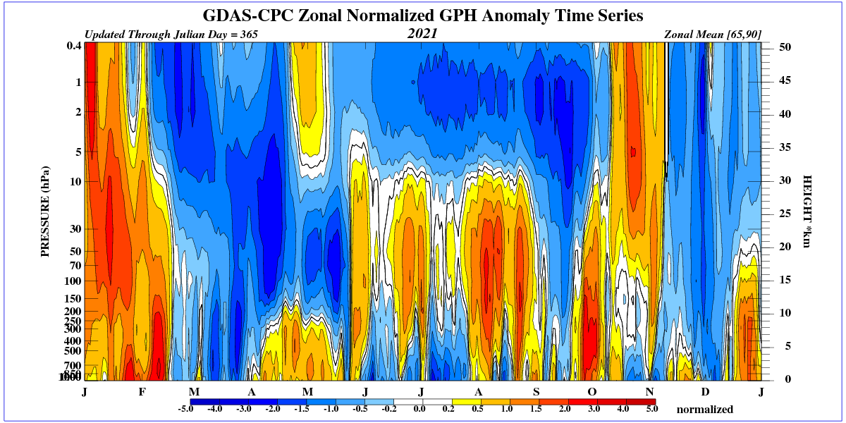
As a result, snowfall can be expected to increase in the northern hemisphere because the oceans in the northern hemisphere are quite warm.
http://globalcryospherewatch.org/state_of_cryo/snow/fmi_swe_tracker.jpg
High permanent SOI heralds the development of La Niña, which will result in lower winter temperatures in the troposphere in the northern hemisphere. This is an additional argument for increased snowfall.
https://www.longpaddock.qld.gov.au/soi/
It is worth asking why the equatorial Pacific remains cool, and how long will this continue?
http://www.bom.gov.au/archive/oceanography/ocean_anals/IDYOC007/IDYOC007.202107.gif
If we see high ocean surface temperatures in the Northern Hemisphere, it is important to remember that the Earth is closest to the Sun in orbit in January.
Dearest Ren, what is an SSW pray tell?
It tells me to sit in ZEN and embrace the cosmic energy.
Sudden Stratospheric Warming
The SSW mechanism is speculation to me. It is clear to me that the phenomenon occurs in the stratosphere and gradually moves to lower layers in the polar vortex. Planetary waves? Certainly, but they are created already in the mesosphere.
Slow Solar Wind.
Ren is like a Zen master. You can try to get wisdom out his words, but you won’t get useful answers to your questions. Lol.
In a relatively short amount of time, NASA’s SORCE mission proved that solar radiation at different wavelengths did not change in lockstep with TSI. Just as CO2 affects certain wavelengths of outgoing radiation, certain wavelengths of incoming radiation are reflected by the atmosphere.
It is possible for TSI to be completely constant while changes in the mix of radiation along the solar spectrum could account for all warming since 1900. Or TSI can have moderate changes without causing any noticeable changes in temperature. We simply do not have enough data.
Given the failure of many RF/GHG precitions as well as inability to predict long term past I am sceptical that solar RF is the correct measure of climate variability.
TSI is not what warms the skin or what gives a sun burn. TSI is not what affects radio communication. Yet all are affected by sun.
GHG has resulted in tunnel vision.
Agreed. Arguing within the framework of RF and ECS is far too confining. Climate is much more complex than that.
“TSI is not what warms the skin or what gives a sun burn. TSI is not what affects radio communication”
Since TSI includes ALL the radiation the Sun outputs [that is the T in Total Solar Irradiance],you are claiming that sun-burns and Radio-Interference are NOT caused by anything the Sun radiates. Think about it for a second. What are the causes then, if not something the Sun radiates?
Most of us cannot predict what the bathroom scale will read in the morning even when we know what we had for dinner the night before.
We can only predict the orbits of the planets because they lie in a plane. Our mathematics breaks down otherwise.
A similar problem exists for solar prediction. Unless the attractors (dimensions) lie in a plane – no reason they should – the error term will grow faster than rhe result.
This is often overlooked because humans assume there will be positive and negative error that will average out to zero. Only true for limited class of problems.
For example drive a car blindfolded. Will your plus minus drift average out to zero?
“We can only predict the orbits of the planets because they lie in a plane. Our mathematics breaks down otherwise.”
That statement is obviously false:
1) Referenced to the plane of the ecliptic (the plane in which Earth orbits the Sun), the seven other major planets have orbits variously inclined by 0.77° (Uranus) to 7.01° (Mercury), and the minor plant Pluto is inclined at 17.14°. None are coplanar. (ref: https://en.wikipedia.org/wiki/Orbital_inclination )
2) With the advent of modern high-speed digital computers, solution of n-body gravitational equations became quite easy for any arbitrary configuration of planetary orientations and any number of non-coplanar orbits. This is exemplified by the precise celestial navigation employed by NASA on all of its spacecraft missions to explore planets, the moons of planets, asteroids, and to even intercept comets within the solar system. “Our mathematics” do not break down, but instead serve us extraordinarily well in such cases.
We look at science 500 years ago and think how primitive and ignorant. 500 years from now science will view us the same way.
500 years ago the learned men of their age took great pride in how much they knew with no knowledge of how much more they didnt know.
This age is no exception. We dont know how much we dont know.
As already mentioned, for the Sun to be the dominant (that is >50%) cause of recent warming, the Sun would have to increase its output about 6 W/m2 since 1750, or 0.02 W/m2/yr on average.
==========
Not correct. That assumes only TSI affects temperature.
A small change in clouds could have the same affect. Only 1 example of many possible.
And what about meander? Why assume temperature will follow a straight line when water and air do not? Assuming facts not in evidence.
Ferdberple,
I acknowledge, in the post, that solar variability can affect our climate in other ways besides TSI. Also, there are many other things that affect climate, like cloud cover, I’ve written about that elsewhere. This post was specifically about TSI, as clearly stated in the post.
A recent post of mine on clouds can be see here:
https://andymaypetrophysicist.com/2021/04/28/clouds-and-global-warming/
I’m a firm believer is writing only about one thing at a time; I detest going off on tangents.
TSI affects the amount of cloud cover. Cloud cover was highest in the modern era after the highest solar activity and has been reduced after lower solar activity.
http://climate4you.com/images/CloudCover_and_MSU%20UAH%20GlobalMonthlyTempSince1979%20With37monthRunningAverage%20With201505Reference.gif
the gradient of tropopause height between equator and poles
≠========
Air flows downhill just as does water. This explains convection and the lapse rate as a result of differential heating between equator and poles.
Simple question #1: does relatively hotter air flow “downhill” into relatively colder air?
Simple question #2: does air experience a centrifugal force difference that occurs naturally between the equator and the poles of the rotating Earth?
Can we predict grouped declines and increases that appear to be more important for climate?
Can we predict long-term solar variability?
Yes. Venus, Earth, and Jupiter are the dynamo, but the absolute timing of each sunspot cycle maximum is ordered by heliocentric Earth-Venus inferior conjunctions in syzygy with Uranus, and in syzygy or in quadrature with Neptune during centennial solar minima sunspot cycles.
https://www.linkedin.com/pulse/schwabe-cycle-variability-ulric-lyons
Andy May:
“what Svalgaard and many other astrophysicists believe, is that by keeping track of the larger sunspots and sunspot-related features in the Sun’s photosphere, they can detect all significant solar variability”
No, that is not true. Magnetographs detect the total magnetic flux through the instrument aperture including from features that are not sunspots of related to sunspots. So, the quiet areas are measured as well. In, fact, those make up most (like 90%) of the flux. We can also measure directly the temperature from quiet regions with no visible spots or activity. E.g.
Large-scale Structures and their Role in Solar Activity ASP Conference Series, Vol. 346, 2005 K. Sankarasubramanian, Matt Penn, and Alexei Pevtsov Quiet Sun unaffected by Activity Cycle W. Livingston1 , D. Gray 2 , L. Wallace3 , and O. R. White4
Abstract:
The Sun’s 11 year sunspot cycle, and all related phenomena, are driven by magnetism in the form of hot flux tubes which thread through the surface from below. Full disk chromospheric Ca K intensity observations track the activity cycle. But center disk Ca K and photospheric temperature sensitive lines are invariant to cycle magnetism. Recent high resolution photographs of the photosphere show that the flux tubes are confined between the granulation cells and do not interact with them. The result is a constant basal atmosphere without cyclic consequences for the Earth.
Therefore, there is no evidence for Q-regions heating the photosphere as is the basic premise for asserting that such heating is the cause of large variations of TSI.