Guest Post by Willis Eschenbach
My last two posts, one on Gavin’s claims and the other on the Urban Heat Island (UHI) effect, have gotten me to thinking about the various groups producing historical global surface temperature estimates. Remember that the global surface temperature is the main climate variable that lots of folks are hyperventilating about …
In particular, in the earlier post, Steven Mosher has been defending how the Berkeley Earth folks handle the Urban Heat Island effect. I remembered that Berkeley Earth had data about cities, so I went and got it from here. The data shows the trends for the period after 1960.
I graphed it up, but I wanted to have something to compare it to, so I also got the data for Berkeley Earth global surface temperature trend since 1960. Figure 1 shows the result:
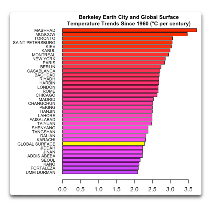
Figure 1. Berkeley Earth trends for various cities, along with the global surface temperature trend over the same period.
There were a couple of things that I found unusual about this. First, there are some indications that the Berkeley Earth method of removing the Urban Heat Island distortion of the global temperature record is … well … perhaps not all that accurate. However, more research would be needed to determine that.
The bigger surprise to me, however, was the size of the Berkeley Earth global surface temperature trend. I had remembered the global trend as being around two-thirds of the value shown in Figure 1. I thought “Over two degrees per century? That’s over two-tenths of a degree (0.2°C) per decade! How did it get that high?”
The answer is, that’s land-only Berkeley Earth data … the global Berkeley Earth data is less than that. A lot less.
So, being addicted to data, I went and got the temperature records from a variety of organizations. I wanted to include the satellite-measured temperatures of the lower troposphere, which only started in 1979, so my analysis covered 1979 to the present. I got the data from Berkeley Earth, the Hadley Centre (HadCRUT), the Goddard Institute of Space Sciences (GISS LOTI), Remote Sensing Systems (RSS), the University of Alabama Huntsville (UAH) and the Japan Meteorological Agency (JMA). I smoothed them all with a 6-year Gaussian average and graphed them up.

Figure 2. Surface and lower troposphere temperature records from six different groups.
For me, the best part of science is my first look at some batch of numbers that have been converted into a graph. It’s always so exciting waiting for the unknown surprises. In this case, I cracked up laughing when I saw the graph. If there were ever an indictment of the current state of climate science, it’s shown in that graph.
People are all up in arms about the surface temperature … but thirty years after James Hansen started madly beating the alarm bell about “global warming”, and after thirty years of endless claims about some mythical “97% scientific consensus”, the sad truth is that the climate scientists have not even been able to come to a consensus regarding how much the globe has warmed in the last 60 years. I mean, the answers differ by a factor of 1.5 to 1!
And mainstream climate scientists wonder why people don’t pay much attention to them? …
Here’s a protip. It’s not a communications problem. If you want people to listen to what you say, first you have to centralize your fecal material.
My best wishes to everyone,
w.
My Usual: Please quote the exact words that you are discussing in a comment. Otherwise, we can’t tell what you are referring to, and misunderstandings multiply.
The best data is the worst and that’s by design.
Berkeley [Earth] represents the worst case scenario. Mama, don’t let your babies grow up to be …
Climate scientists.
Mamas, don’t let your babies grow up to be “Hansens”
Don’t let ’em pick cherries or adjust them old charts
Let ’em be honest with ethics and such
Mamas don’t let your babies grow up to be “Hansens”
‘Cos they’ll say anything to promote that ol’ “Cause”
Even to someone they love
MODS, I made a reply that hasn’t shown up. ( I did wait awhile.)
It was spoofing the chorus to “Mama, don’t let your babies grow up to be …”.
I suspect it went to auto-bit-bin because I used the word fr@ud. “But I didn’t say ‘Fudge'”.
(I did not use in reference to an individual.)
Thanks.
Guess I didn’t use the F word after all.
(But it would be applicable!8-)
Anyone who starts out calling a project BEST before they even have the data, has a hubris problem.
I was prepared to keep an open mind about Muller while he had Curry and Watts on board. When he pulled to rug on the collaborative effort, he lost the credibility he may have had.
Why doesn’t anybody note that the Average Daily Temperature of the Continent of Antarctica is 59 degrees BELOW Zero F? WE keep hearing how the warming is going to melt that South Pole, but NO ONE ever tells us how 5-10 degrees of warming is going to accomplish this “miracle”. Where are all the scientists with an explanation for a simple question?
See Clive Best for a gridded global approach
http://clivebest.com/
Organize the cities by Latitude? That might also be interesting.
And altitude. Mashhad and Kabul are near the top of the list and are 1,000 and 2,000 metres ASL. They are near the top of the list along with “cold country” cities.
YUP”, the Figure 1graph may be accurate, …… but highly misleading.
The literal fact is that near-surface temperatures are highly dependent upon both the altitude and latitude that they are recorded at. And to get real persnickety about it, longitude is also a critical factor, to wit:
New York City —– 40.7128° N, 74.0060° W
January — 39° / 26°
February – 43° / 29°
March —- 52° / 36°
April —– 64° / 45°
London England —– 51.5074° N, 0.1278° W
January — 48° / 40°
February – 49° / 40°
March —- 53° / 42°
April —– 59° / 45°
A 10.7946° difference in latitude ….. but nearly identical average temperatures.
If not for the Gulf Stream, ….. Great Britian would be as cold as Hudson Bay.
Looks like they are already sorted in latitude. That was the first thing which struck me.
Don’t take it too literally but the top ten ( with the exception of Kabul ) are pretty much in latitude order.
Also , despite Aus being this years “canary in the ever moving coalmine” , I don’t see anything south of Seoul in the list.
In my eyes they are sorted by temperature trends value, not by latitude.
Or it’s the same order 😀
I recommend you add JRA-25 and ERA-5 2m and 850mb, 700mb and 500mb to your assessment.
Why are the 1980 data clustered so closely together relative to the present day data?
Tom, to answer your question, the base period for anomalies, according to Willis’s graph in his Figure 2, is 1979-1985.
It’s a logical choice, in this case, because he wants to show how the datasets diverge with time.
Regards,
Bob
Thanks. I should have thought about that a little harder…
It occurs to me that maybe the base period should be close to the present instead, and we should look at where the data starts. After all, it’s been pointed out here many times that certain “adjustments” have been made to historical records which amazingly all seem to be going in the same direction. So we should see how cold it really was in 1960, should we not? Some of us were even around at the time.
Absolutely, yes. The best data we have are USCRN, and that data is only contiguous over the last ~10 years.
By all means, set every base period as 2008 forward until we have a full 30 year base, then let it slide forward each year.
It might shine a new light on all the nutty adjustments being added to the past and present.
The total effect is largely in the ‘adjustments’ methinks.
GlobalTemperature =
Solar Effect+Cloud Effect + Greenhouse Effect + Heat Island Effect (Urban and other anomalous) + Instrument Relocation Effect + Instrument Technology Change Effect +
Location-Area Adjustment Effect + UHIAdjustment Effect + MaintainUptrendEffect + HeadlineChasingAdjustmentEffect + 97%ConcensusAdjustmentEffect + DenierBashingAdjustmentEffect
There is also a puzzling divergence from 2000 in the HADCRUT4 NH mean and SH mean:
http://woodfortrees.org/plot/hadcrut4nh/mean:12/plot/hadcrut4sh/mean:12
It surely needs ‘adjusting’.
A bit like their models and their ETS and TTS etc.
Of course the science is settled.
The only thing that’s really settled are the solutions. Everything else is backfill.
That’s exactly what is wrong with the whole global warming thing:
it’s a solution in search of a problem.
The solution being abolishing democracy and establishing global government (i.e. communism). The problem is non-existing but it sounds so good and people want it to be true. It’s trust-abuse. 97% agree, remember?
Which UN biggie was quoted as saying that it didn’t matter whether global warming was true or not, because it forced people to do things that needed doing anyway?
“We’ve got to ride this global warming issue.
Even if the theory of global warming is wrong,
we will be doing the right thing in terms of
economic and environmental policy.”
Timothy Wirth,
President of the UN Foundation
For more devastating quotes, see: http://www.green-agenda.com/
Are those rates statistically different?
Hard to tell … but when they differ by a factor of two to one, they’re practically different, particularly in the effect that they have on the overheated debate.
w.
Yes. I agree. All of these methods of assessing gmst seem weak to me.
Another fine job, Willis, but dammit, I did it again.
You see, at an early age I thought it might be cool to have a large vocabulary and true to form, just looked up surfeit.
Problem is, now I’ll use the word all over the place, because I’m smart enough to understand it, but not smart enough to not use it, so end up sounding like an academic a*hole, instead of the regular kind.
It’s a sister to forfeit or forfait
Or even ‘surfait fait’
in re my prior comment: Use of surfeit in this forum is naturally apropos and shows that Willis knows how to get ‘er done, while I typically pick up the wrong bat.
Willis
“People are all up in arms…”, “hyperventilating”
“mainstream climate scientists wonder why people don’t pay much attention to them”
“cracked up laughing when I saw the graph.”
You pour scorn and derision on climate science but then it appears in your haste to cast doubt you yourself have produced a bit of “fecal matter” – “the answers differ by a factor of 1.5 to 1!” Nick’s graph below appears to totally refute this.
Are you standing by your ridicule?
Crickets.
“Are those rates statistically different?”
The 95% CI range for the AR(1) trend for GISS from Jan 1979 to Dec 2019 is 0.166 to 0.21. So the differences between land/ocean measures are not statistically significant. The differences between land/ocean and lower trop, or land/ocean and land only, are significant.
AR(1) is merely a mathematically convenient, a prori model for surface temperature variations. Empirically, it’s a gross fiction. Check out the stark differences in spectral structure.
Analysis is done here, mainly by acf, with some spectra also here. The main deviation from AR(1) is an unexpectedly large oscillation in the series.
How would you suggest estimating the confidence range? Do you think it would alter the conclusion that the land/ocean trends are not significantly different, while the trends of different kinds of data are?
Don’t estimate stuff that can’t be estimated. You end up with specious results.
Isn’t that obvious.
The “unexpectedly large oscillation” provides ample proof that the acf of surface T doesn’t resemble structurally the monotonically declining, non-negative acf of AR(1). And the (hanned) power spectrum of GISP2 Holocene data clearly shows significant peaks of various bandwidths that are irreconcilable with AR(1). See: http://i1188.photobucket.com/albums/z410/skygram/graph1.jpg
The realistic way to estimate the confidence intervals for such complex processes is via Monte Carlo simulation, rather than academic presumption.
Nick,
To quote those figures for 95% C.I. range, one might assume that there is a peer reviewed paper disclosing method of calculation, data sources, assumptions and so on. Please f this is so, what is the reference?
I have been rebutted for several years by your BOM after repeatedly asking for their similar figures for their routine temperature data, more primary than your AR(1) trends, with their responses seeming to insinuate that it is too complicated to reduce findings to a simple number or two.
I am particularly interested in how the AR(1) number analysis treats the uncertainty calculations for invented, guessed T where T numbers now exist in places distant from the nearest measurements. Geoff S
Geoff,
The data is just the published time series, same as Willis is plotting. The methods are fairly standard, and are described in detail here and here.
“where T numbers now exist in places distant”
The trend uncertainty is calculated for the time series of global averages, and uses the observed apparent variance. The uncertainty due to location belongs within the global average, and is appropriate if you need to assign an uncertainty to those figures.
Nick,
It’s my understanding that Confidence Interval is a statistical measure and does not reflect the full uncertainty in the global temperature estimates. From what I recall, HadCRUT presents a monthly uncertainty derived from an ensemble approach for estimating uncertainty, although my subjective feeling is that their uncertainty estimates are still too low.
I also recall that you have done quite a bit of work as presented on your blog about different methods for compositing (integrating) global temperature measurements to produce an estimate of global temperature anomalies. From what you have presented, it seems to me that much of the differences between the estimates from various agencies are more from the integration method and handling of data sparse areas than anything else, since they all use slightly different methods in these regards. This is especially true in the Arctic area where probably most of the warming has occurred in recent decades and mainly in the Arctic winter (Arctic night) and that is a data sparse area with large high temperature anomalies that could drive much of the differences.
For instance, HadCRUT tends to be on the lower end of the global warming estimates and from what I recall, they do not attempt to estimate temperature anomalies in grid cells where measurements are not available. Thus much of the Arctic region, being data sparse, is essentially not included which effectively assigns these areas equivalent to the global average, which probably causes a low bias.
Most of the groups, except BEST from what I recall, use NOAA’s GHCN homogenized monthly surface air temperature measurements for land in conjunction with gridded sea surface temperature estimates based on ship and buoy data and may or may not include satellite sea surface temperature estimates. More room for discrepancies, depending on the choices made. I also recall that you have produced estimates using the raw GHCN data in conjunction with ERSST sea surface data and using a variety of integration methods.
As far as urbanization effects, I’m still not convinced that any of the current homogenization methods provide a very accurate removal of the these effects. I call it “urbanization” rather than “urban heat island” because urbanization effects can occur even at relatively rural sites. What is important are the changes over time, which can be very localized urbanization such as construction of a building or paved parking area near the monitor, or on a larger scale from slowly encroaching suburban and/or urban development over a nearby range of one to 10 km or more. I suspect this effect is not especially large on a global scale, but could possibly account for a significant portion of the man-made influence on recent global warming. I recall an important study that Anthony Watts et al conducted examining station siting issues that could affect temperature anomalies if there have been significant changes over the time scales of interest. If there are no changes in siting issues and/or other urbanization effects over time, then there should be little effect on temperature anomaly trends over that time period.
Bryan,
“does not reflect the full uncertainty in the global temperature estimates”
The CI for a time series trend reflects a probability model fitted to the numbers. It does not try to work out the underlying sources of error. Because they are based on a large number of readings, it is expected that random error variation in the underlying data will be reflected in the standard error of the weighted mean, which is the trend.
“From what you have presented, it seems to me that much of the differences between the estimates from various agencies are more from the integration method and handling of data sparse areas than anything else, since they all use slightly different methods in these regards.”
Yes, that is true. The first requirement of a good method is that you make a proper estimate for all the data; not leaving patches out. If you do that, then while it is possible to improve the integration method, it won’t make a huge further difference.
“More room for discrepancies, depending on the choices made. I also recall that you have produced estimates using the raw GHCN data in conjunction with ERSST sea surface data and using a variety of integration methods.”
Yes, that is true too. I quoted above the trend for TempLS, which is based on unadjusted GHCN. For that period it was almost exactly the same as NOAA and HADCRUT. In fact I think they have a slightly lower trend because of weak treatment of the Arctic (cf C&W), so the corresponding reduction in TempLS could be attributed to using raw data. It is not nothing, but not much.
“I recall an important study that Anthony Watts et al conducted examining station siting issues that could affect temperature anomalies if there have been significant changes over the time scales of interest.”
It’s worth bearing in mind here the very close agreement between USHCN, USCRN and ClimDiv for ConUS for the period since 2005. Since USCRN has good, non-urban stations then if UHI or siting are having an effect, it must be an unchanging effect over that period.
Nick,
Call me a conspiracy therorist, but as I read here ( ? memory may be faulty) but the USHCN las been suspended since the USCRN came on line.
They are now forced to be the same by the powers that be, since the USCRN is unimpeachable and cannot be “adjusted”.
And over the history of the USCRN (which deserves better press coverage) there is NO discernible warming. Though not global in its reach, it does indicate that the changes in US temperatures are not dangerous or scary.
“but the USHCN las been suspended since the USCRN came on line”
Memory is faulty. USHCN was replaced by ClimDiv in 2014. Both have a substantial overlap with USCRN. And they all agree very well.
a_scientist
“And over the history of the USCRN (which deserves better press coverage) there is NO discernible warming.”
AHA.
Of course we can’t expect very relevant trend info when we inspect a time series averaging about 200 stations over a period no longer than 15 years.
Nevertheless, the linear estimate for the average of the raw data of all CRN stations during 2004-2019 is: 0.34 ± 0.18 °C / decade.
*
“Though not global in its reach, it does indicate that the changes in US temperatures are not dangerous or scary.”
Indeed. But… the US are 2 % of the Globe’s surface.
Rgds
an_engineer
UHI and other land-use effects cannot be meaningfully assessed from records only a decade or two long. The presence of strong multi-decadal oscillation requires records at least an order of magnitude longer for SECULAR trend differences to emerge. The inability (or unwillingness) to cope with this fundamental analytic requirement renders all sanguine conclusions drawn from short records quite meaningless. Their apparent linear trends are themselves oscillatory, rather than steady.
Bryan – oz4caster
“I recall an important study that Anthony Watts et al conducted examining station siting issues that could affect temperature anomalies if there have been significant changes over the time scales of interest. If there are no changes in siting issues and/or other urbanization effects over time, then there should be little effect on temperature anomaly trends over that time period.”
This is a major point into which I focused by performing a little experiment last year.
NOAA published years ago on this page:
https://www.ncdc.noaa.gov/ushcn/station-siting
a list of 71 USHCN stations acknowledged as well-sited by Anthony Watts’ surfacestations.org:
ftp://ftp.ncdc.noaa.gov/pub/data/ushcn/v2/monthly/ushcn-surfacestations-ratings-1-2.txt
All these 71 stations exist within the GHCN daily station set
ftp://ftp.ncdc.noaa.gov/pub/data/ghcn/daily/ghcnd-stations.txt
as well, so I compared them with GHCN daily’s entire CONUS subset:
https://drive.google.com/file/d/1pbQCHFwTTy1HIns9pDNj6mDQ85Vau7NC/view
As you can see when looking at the running means, the 71 ‘well-sited’ stations show a slightly higher trend than the average of all (over 8000 actually) stations located in CONUS (AK wouldn’t change much).
I did the same with these ‘pristine’ CRN stations, by comparing the average of all CRN stations (about 200) available in GHCN daily with all CONUS stations:
https://drive.google.com/file/d/1zg9M-GZwNoIBln404Ay0voAL8V4PmSdK/view
Here too, we see that the discrepancies are minimal.
Of course: despite it was subject to heavy V&V, this GHCN daily data processing is and remains layman’s work.
Feel free to do the same job and compare the results 🙂
Rgds
J.-P. Dehottay
Bindidon,
Thanks for sharing your two graphs. I also looked at the graphs provided by NOAA, where they use a gridded model to produce CONUS annual temperature anomalies for comparing USHCN, USCRN, and nClimDiv. They used a baseline for the anomalies that was prior to the start of the USCRN and used relationships with nearby stations to estimate a baseline for the USCRN. Their results are similar to your second graph.
While some sites probably do have significant urbanization changes over time, the amount is likely to be variable from one site to another and for different time periods, adding complexity. However, in areas like CONUS and Europe the station density is so high now that any effects may hidden in the noise. In areas with low station density, urbanization effects could potentially play a larger role in influencing regional temperature anomaly trend estimates, especially for sites in or near rapidly growing urban areas that show steady long-term population growth encroaching around the sites. Regardless, I doubt the effect is very significant on a global basis, but it may not be negligible for land only temperature trend analyses and especially for some regional and local trend analyses.
You did anomalies not temperatures.
The urban heat island effect certainly does not look to have been removed from those cities, and exactly how much corruption by spreading that temperature over thousands of square miles and homogenizing it with rural datasets raises the average?
Berkeley BEST is just another group of warmists.
I remember when they were first brought forward, they were going to be the good guys, and they were going to correct the lies. It seems as though they have amplified the lies.
Good cop, bad cop
EPA used to have a lot of stuff up about UHI, they say temp changes are a whole lot more than what Berkeley claims…
EPA > “. The annual mean air temperature of a city with 1 million people or more can be 1.8–5.4°F (1–3°C) warmer than its surroundings. In the evening, the difference can be as high as 22°F (12°C).”
https://www.epa.gov/heat-islands
====
ex: EPA says a +15 degree difference between rural and city Atlanta > https://www.epa.gov/sites/production/files/2014-07/documents/epa_presentation_oct05.pdf
Heck, this morning there was a 41 F difference in temperature between Traverse City, MI and Grayling, MI. They are only about 55 miles apart and almost directly east/west from each other. That is one of the largest differences I have ever seen with cities that close together.
What happened in 2000? Irrespective of whether the numbers are in any way connected to reality, they are reasonable coordinated for the first 20 years, then in the year 2000 they diverge wildly, and the last 20 years they go their own way. What happened?
Looks to me like the longer the analysis, the more the divergence…tough to diverge wildly close to the beginning.
Ron
There was the massive El-Nino-La Nina event from 1997-1999, which shifted a few million cubic km of warm sea water from the equator toward the poles, perturbing global climate and raising global temperatures as Bob Tisdale has explained in previous posts.
“What happened in 2000? Irrespective of whether the numbers are in any way connected to reality, they are reasonable coordinated for the first 20 years, then in the year 2000 they diverge wildly, and the last 20 years they go their own way. What happened?”
In 1998, the global temperatures reached the warmest year since the 1930’s.
The CAGW proponents back in the 1980’s claimed human-caused global warming was going to cause the temperatures to increase and their predictions were correct right up until around the year 2000. The beginning of their claims for CO2 warming were in the 1970’s, one of the coldest periods in recent history, so it was not much of a stretch to say the temperatures would probably climb from there.
And the temperatures did climb right up to the El Nino high of 1998, so the CAGW proponent’s predictions were proceeding along the way they predicted but then the warming stopped, and the cooling started, so that was about the time the CAGW proponents thought they needed to bastardize the global temperature record some more in order to make it look like things were getting hotter and hotter year after year, instead of flatlining or cooling.
During this time they turned 1998 from the warmest year since the 1930’s into an insignificant year.
They did this so they could claim that the years following 1998, were the “hottest year evah!” in order to continue the CAGW narrative. As you can see below, if they had used the UAH satellite chart instead of the fraudulent Hockey Stick chart, they couldn’t make the claims that six or eight years in the 21st century were hotter than 1998. UAH shows only one year was hotter than 1998, and that was 2016, which was one-tenth of a degree warmer than 1998, a statistical tie.
Note how the fraudulent Hockey Stick chart eliminates the warmth of the 1930’s and the cold of the 1970’s and the warmth of 1998. It’s a bastardized temperature record created to push a political/personal agenda.
Fraudulent Hockey Stick chart:
UAH satellite chart:
http://www.drroyspencer.com/wp-content/uploads/UAH_LT_1979_thru_December_2019_v6.jpg
There are two confounding factors within these data. If the BEST global surface trend is from land+ocean, then any data from land sensors, such as cities would be hotter than the ocean. Also, as Clive Best (not related) showed, anomalies such as these are biased by the higher volatility at higher latitudes.
Ron Clutz
Correct!
“What happened?” Desperation kicked in.
markl,
+1
Hi Willis,
(1) Zoe Phin posted these yesterday regarding BEST. Thoughts?
https://phzoe.wordpress.com/2019/12/30/what-global-warming/
https://phzoe.wordpress.com/2020/01/17/precipitable-water-as-temperature-proxy/
(2) “… I smoothed them all with a 6-year Gaussian average and graphed them up…”
In the graph it looks like 3 end in 2020 (i.e., through 2019), 2 end in 2019, and BEST ends 2017?
Brilliant!
Equation (1) in http://globalclimatedrivers2.blogspot.com produced a match of 96.7% 1895 to 2018 with 5-yr-smoothed measured average global temperature by accounting for water vapor (Total Precipitable Water), SSN and the net effect of all ocean cycles approximated by a saw-tooth profile with 64 yr period. IMO the clouds are accounted for with the SSN anomaly time-integral (sort of like Svensmark). The equation divvies up the ~0.9 K temperature rise since 1909:
sun 17.8%,
ocean 21.7%,
WV 60.5%.
I see that I’ve used the Berkeley Earth land data instead of the land+ocean data … corrected now. The spread is less but the point remains … the spread in the results is far too large.
w.
Willis
The inclusion of ocean temps damps the variation because of the large difference in specific heat. Cities are on land. Why would you want to compare them with ocean temps? I think that you did it the right way the first time.
Clyde, land cities are compared to land temps in Fig. 1.
Global temperature records are compared to global temperature records in Fig. 2.
w.
Willis,
Are you using the correct data for other data sets?
I’ve looked at my downloaded data using the same base period as you, and I cannot see how GISS is warmer than RSS. It should be very close to BEST unless I’m doing something wrong.
I also cannot see how HadCRUT is now below JMA.
Bellman
Correct! JMA has a much lower trend than all other surface series. It is partly deue to lack of interpolation, what imho is particularly noticeable within their COBE-SST2 sea surface stuff.
And GISS has indeed, as you wrote below, a trend of 0.19 °C / decade.
“how GISS is warmer than RSS”
Yes, I got 0.188 °C/decade for GISS and 0.208 °C/Decade for RSS. Incidentally I made a small mistake with trends quoted earlier, in that I requested 1979-2019, but that gives a result ending Dec 2018, so the last year is missing. Since 2019 was warm, the full trends are about 0.004 °C.decade higher, but the order doesn’t change.
Here’s my attempt at a similar graph
There definitely seems to be something wrong with the ends of the graph in the head posting. GISTEMP should be below RSS, and very close to BEST. JMA is currently almost identical to UAH and HadCRUT is somewhere between GISTEMP and JMA.
Willis,
You are still exaggerating trend differences. The Gistemp trend 1979-2019 is 0.19 C/decade, not 0.21.
The HadCRUT4, NOAA, and JMA datasets have coverage bias, JMA also lacks the ship/buoy adjustment.
RSS has a slight warm bias, avoiding most of cool Antarctica.
The true and only outlier is UAH, but their analysis of microwave radiances is subjective, since they have made significant choices and adjustments not supported by data
Datasets that are apples to apples, decadal trends 1979-2019:
Berkeley l/o 0.189
Gistemp loti 0.188
Cowtan&Way 0.187
Very good agreement, right?
Willis,
“For me, the best part of science is my first look at some batch of numbers that have been converted into a graph.”
You can make such a plot interactively here. And here is a snapshot. The agreement is much better than you say.
” I mean, the answers differ by a factor of two!”
Well, it helps if you are comparing the same thing. Your highest is Berkeley land only. The lowest is UAH lower troposphere. If you split them into groups according to what they are measuring, I get, from 1979, in °C/decade:
Land/Ocean:
BEST 0.186
GISS 0.184
HADCRUT 0.170
NOAA 0.170
TempLS 0.169 (My own calculation)
Lower Trop
RSS 0.204
UAH 0.127
Land only
BEST 0.282
The variation factor for land/ocean is 1.1, not 2.
Thanks, Nick. I already noticed that and fixed it. My point remains. Look at the differences, not just in the trends, but in the patterns of the changes in each one. It’s a pit of unrelated snakes. Wildly different.
In any other science what they’d likely do is select a group of experts to examine each of these and determine a) why there are differences and b) what can be done to bring them into harmony.
In climate science, on the other hand, groups just each make their own claims and keep going.
Finally, I appreciate you (and many others) checking my work. It’s one of the beauties of writing for the web—my errors get pointed out in record time.
w.
Willis,
” It’s a pit of unrelated snakes. Wildly different.”
It isn’t if you compare apples with apples. Here is a plot of just land/ocean indices. I have replaced HADCRUT with the Cowtan/Way index, since that is a case where scientists identified the issue causing discrepancy and corrected it. It is more like a pit of mating snakes. It uses 12 month running means of monthly data.
Thanks, Nick. I don’t understand that. It looks like land-only. Is that correct? Also, a boxcar filter like you’ve used is a bad choice … I’ve posted your graph in-line for ease of discussion.
w.
Willis,
Thanks for posting. The plots are land/ocean. The trends are as shown in my comment above, but in C/Cen units. The boxcar filter for smoothing monthly to annual will give similar results to others, and won’t create agreement where none existed.
I made a mistake in requesting the trends here and got 1979-2018 instead of 2019. Since 2019 was warm, trends for 1979-2019 (inclusive) are a little higher:
Land/Ocean:
BEST 0.188 C/decade
GISS 0.188
HADCRUT 0.172
NOAA 0.173
TempLS 0.173 (My own calculation)
Lower Trop
RSS 0.208
UAH 0.132
Nice work Nick, you eliminated the data sets with the most discrepancy ( without comment ) and replaced the third lowest with a “corrected” version.
I suppose you have to pick cherries if you want to make cherry pie.
Greg,
“you eliminated the data sets with the most discrepancy”
As I said several times, I gathered the sets that were actually measuring the same thing – land/ocean surface temperature. The discrepancy with the LT sets is not an issue of measurement; it is a different place.
Not that there are no issues of measurement. The surface measures largely agree,; one LT set is above them all, and one below.
“replaced the third lowest with a “corrected” version”
In the spirit of Willis’
“b) what can be done to bring them into harmony.”
The reason for the error of HADCRUT was identified and corrected.
Agreed , TLT is in a different place. As land and sea are different places. Why the hell anyone would want to take the “average” of sea and land air temps and pretend it has physical meaning is beyond me but it seems to fashionable because it warms more.
If TLT is rising less than pseudo surface average temps you need to explain why before concluding it is “not an issue of measurement”.
If there was an “error ” in HadCRUT, Had and CRU would have corrected it. The “error” is that they use the data they have instead of including zones where they don’t have data.
reg,
“and pretend it has physical meaning is beyond me but it seems to fashionable because it warms more”
People have carefully tracked how the air just above the sea closely tracks SST. SST is used because we have a better history. It actually warms less than land only, and also less than the extended land that GISS started with and maintained until last year.
“If TLT is rising less than pseudo surface average temps you need to explain why”
No, you don’t. It’s just an observation of two different places. Just as sea warms more slowly than land.
“The “error” is that they use the data they have instead of including zones where they don’t have data.”
No, they are failing to use the data they have. To get something you can call global temperature you need your best estimate of every point on the globe. Every point where you don’t actually have a thermometer is an estimate. HADCRUT’s error is that they apply an arbitrary grid, and then assign to cells a temperature equal to the average of the remainder. That is what simply omitting
empty cells does. It is much inferior to an estimate based on nearby information, which is what is used everywhere else.
“best estimate” is not Data.
Just as the “Average” daily or monthly is not the mean and loses very important information.
But of course it tells the required story when you torture it enough.
Greg,
Do you think that is the case? There are two TLT data sets, one shows temp rising faster than global surface temp, the other less. Why do you choose to accept one of those data sets and disregard the other?
40 years strait up, the grapf is a work of art, I have to try harder.
This graph is a perfect example of why I keep saying that arguing about the error bars is a red-herring, and a lost cause.
I can clearly see the ’98 El Nino spike. But… and I have been monitoring this website for a long time… I clearly remember the huge temperature drop followed then the long plateau with essentially no rise for ~15 years. Now, this graph shows the temp matching the ’98 El Nino spike in only 5-ish years. That’s just baloney. That’s not what was being posted back then.
The problem with the data isn’t the error bars… the problem with the data is the data… or rather the constant adjustments in the data. So long as we simply accept those adjustments, we will always be on the defensive.
What was being posted back then? You could try the waybackmachine, though I didn’t have any luck with that myself. I seem to recall seeing temperature exceed the 1998 super el nino year in 2005 and then again a few years later. I think 1997 was a record year, at the time, and that has been exceeded many times. Starting with a super el nino year is bound to make it seem that temperature stalled for a while after that but studies have shown that, statistically, there was not even a slowdown. Of course, data series are revised from time to time as more is learned about interpreting the raw data, so some of the numbers will change over time.
Nick Stokes:
I have just examined your graph with respect to my claim that Earth’s temperatures” are controlled by the amount of SO2 aerosol emissions in the atmosphere, and that the Rule of Thumb, or Climate Sensitivity Factor, is .02 deg of warming for each net Megaton of change in global SO2 aerosol emissions.
Between 1980 and 2014, as near as I can determine , you show an anomalous temp. rise of 0.53 deg C. Between 1980 and 2014, SO2 aerosol emissions fell by a reported 24 Megatons.
Thus, 24 x ,02 = an expected temp. rise of 0.48 deg. C, (within .05 deg. C. of actuality, over a 34 year period. Compare that with projections from any model based upon CO2 !
If NASA GISS Land-Ocean Jan-Dec. anomalous temperatures are used, their reported temperature rise is 0.48 Deg. C., precisely as predicted
In view of the above, how can you continue supporting the “Greenhouse Gas” hoax?
Mr. Eschenbach,
Excellent work, sir. I trust you are amply prepared to give Mosher the “source, codes and data” he will inevitably demand if and when he shows up here? On the other hand, he may choose to ignore your report and article since defending Berkely Earth may be quite difficult for him.
Can I just say, before Mosher gets here, that whatever he says, it won’t even be wrong? I can’t say that? Too late, I’ve said it.
Several months ago there was an article on fitness for purpose about the databases. I came to the conclusion that they are not. I have not changed my mind. Tmax/Tmin/Tavg ends up hiding so much info it’s not funny. Averaging these into bigger and bigger intervals hides more and more info. I never see variances, standard deviations, and uncertainty for the populations of data addressed. I see coastal stations with a data population variance of 5 degrees simply averaged with interior stations with data population variances of 10 or 20 degrees.
If you plot daily T temps for these longer periods by individual cities/rural you get different graphs than averages of large geographic areas. I don’t think appropriate trending theory and tools are applied.
Combining a large number of stations with God only knows what differing uncertainties is asking for trouble. These stations were designed with capabilities for weather forecasting, not for determining regional and global heat values.
And all that is before they make their “adjustments”.
If climate science can’t predict the past what is the hope for predicting the future?
And here is a snapshot of the ever changing temperatures:
https://realclimatescience.com/2020/01/alterations-to-giss-surface-temperatures-from-2001-to-2015/
Thanks , I have a gif somewhere of the changing fortunes of Hansen’s dataset but those newspaper clips from 70s are priceless, almost 0.4 deg. C of cooling in the post-war period, which is now presented as totally flat at best.
“those newspaper clips from 70s are priceless”
And worthless. They are based on a few hundred mostly or all NH, land stations. No area weighting. You are comparing with a modern land/ocean measure.
You missed the whole point didn’t you?
NASA’s records changed, why? Did more stations show up in the period mentioned after they published the 2001 report? Did Nebraska not experience cooling temps during the period? Has NASA appended area weighted temps onto earlier non-weighted temps?
You really don’t explain anything.
You don’t stick to subject. I was responding to “those newspaper clips from 70s are priceless”
Gerald,
The global temperature changes, in the blink of a lie…
Gerald Machnee
What Heller aka Goddard never would tell you is that between 2001 and 2015, considerable amounts of met data was accumulated, especially in the SSt corner, but also for land surfaces.
Let me give you a simple example.
I started processing of NOAA’s GHCN daily in early 2017, after 2 years of using GHCN V3.
While V3 has 7280 stations since around 2010, GHCN daily is growing and growing, moving from ~ 35000 temperature stations in 2017 up to over 40000 in this January.
Do you really think that this has no influence on the global record?
Being fully unprepared for such an increase over time, due to V3 keeping unchanged over years, I unfortunately never kept old data.
What a pity!
Bindidon January 20, 2020 at 4:03 pm
“Gerald Machnee
What Heller aka Goddard never would tell you is that between 2001 and 2015, considerable amounts of met data was accumulated, especially in the SSt corner, but also for land surfaces.”
I was impressed by your information as to the considerable amounts of met data that was accumulated between 2001 and 2015 which enabled NOAA to revise their estimates of global temperatures between 2001 and 2015.
I would have been more impressed if you had also published an explanation as to why so many pre-1940 estimates had been reduced and why so many post-1949 had been increased as a result of the increased number volume of data.
The discrepancies are so obvious that any competent statistician would have investigated
their accuracy before drawing any conclusions as to trends.
Within the bounds of uncertainty, it seems as if the difference between 1.5 and 1 is nil. Whether 1.5 or 1, how much the globe has warmed is indistinguishable from zero, and so, in a strange way, there IS a consensus: How much the globe has warmed in the last 60 years is indistinguishable from zero.
They just don’t know that they are in agreement, and they just don’t know that they are saying this.
It’s funny how the answer can be right before our eyes, and those who determine the answer cannot even understand that they HAVE the answer. It’s zero! Hence, NO GLOBAL WARMING ! [yeah, I’m yelling this time]
How do you get GISS warming at 0.21°C / decade over the last 40 years? I assume you meant 40 and not 60 years. I make it 0.19°C / decade. I don’t think any of the surface based data set trends are statistically different from each other, and the only real deviations are between the two satellite data sets.
The books certainly have been overcooked. It looks like there has been some perverse competition to see who can be the most alarmist; may be linked back to funding?? Which is great for us realists, as they are running out of road to play on before the inevitable crash and burn (they have no choice but to be even more extreme).
Hi Willis,
In the urban areas, does the anthropogenic built environment cause localised reduction of precipitation and surface water infiltration contribute also to urban heat effect?
I ask this because deforestion and mofication of the natural landscape shown to increase temp by 2 to 3 degrees in summer (over thousands of sq kilometers not just a city) and reduce precipitation 10 to 20 % and in some circumstances higher. The Australian deforestation (40% since 1780’s) streches over 3,000 km, down the entire western side of the great dividing range gone.
http://forestsandclimate.org.au/cms/wp-content/uploads/deforestation-and-cleared-land-map-png-1.jpg
Or am i barking up the wrong tree here ?
Willis: “… I smoothed them all with a 6-year Gaussian average and graphed them up…”
It’s very gratifying that you are now an advocate of gaussian filters but how do you padding the 3 years at the start and end ? Those upticks may not be there next time you look. Not a fan of uncleared Mannian padding techniques.
Why do all graphs show a temp decline from 1941 to 1979 while CO2 went up year after year? That is the question that needs to be answered.
T.C
“That is the question that needs to be answered.”
CO2 forcing had not yet overcome the -ve ones of aerosols……
http://www.climatechange2013.org/images/figures/WGI_AR5_Fig8-18.jpg
And at that time the PDO had a sig influence on GSMT …..
http://2.bp.blogspot.com/-Fkg790Q3b8o/VMRGN17t2oI/AAAAAAAAHwo/GTCVnmku248/s1600/GISTempPDO.gif
PDO is based on the difference between N. Pacific and global. If you want to say that was the “cause” of the post war cooling, then it is also the “cause” of late 20th c. warming which is what caused all the end-of-the-world panic. You just removed the final evidence of ANY detectable AGW.
How convenient that the estimate for aerosols cancels the estimates for CO2 for that period.
Your base period of 1979-1985 is too short.