October 4th, 2019 by Roy W. Spencer, Ph. D.
While the vast majority of our monthly global temperature updates are pretty routine, September 2019 is proving to be a unique exception. The bottom line is that there is nothing wrong with the UAH temperatures we originally reported. But what I discovered about last month is pretty unusual.
It all started when our global lower tropospheric (LT) temperature came in at an unexpectedly high +0.61 deg. C above the 1981-2010 average. I say “unexpected” because, as WeatherBell’s Joe Bastardi has pointed out, the global average surface temperature from NOAA’s CFS model had been running about 0.3 C above normal, and our numbers are usually not that different from that model product.
[By way of review, the three basic layers we compute average temperatures from the satellites are, in increasing altitude, the mid-troposphere (MT), tropopause region (TP), and lower stratosphere (LS). From these three deep layer temperatures, we compute the lower tropospheric (LT) product using a linear combination of the three main channels, LT = 1.548MT – 0.538TP +0.01LS.]
Yesterday, John Christy noticed that the Southern Hemisphere was unusually warm in our lower stratosphere (LS) temperature product, while the Northern Hemisphere was unusually cool. This led me to look at the tropical results for our mid-troposphere (MT) and ‘tropopause’ (TP) products, which in the tropics usually track each other. A scatterplot of them revealed September 2019 to be a clear outlier, that is, the TP temperature anomaly was too cool for the MT temperature anomaly.
So, John put a notice on his monthly global temperature update report, and I added a notice to the top of my monthly blog post, that we suspected maybe one of the two satellites we are currently using (NOAA-19 and Metop-B) had problems.
As it turns out, there were no problems with the data. Just an unusual regional weather event that produced an unusual global response.
Blame it on Antarctica
Some of you might have seen news reports several weeks ago that a strong stratospheric warming (SSW) event was expected to form over Antarctica, potentially impacting weather in Australia. These SSW events are more frequent over the Arctic, and occur in winter when (put very simply) winds in the stratosphere flow inward and force air within the cold circumpolar vortex to sink (that’s called subsidence). Since the stratosphere is statically stable (its temperature lapse rate is nearly isothermal), any sinking leads to a strong temperature increase. CIRES in Colorado has provided a nice description of the current SSW event, from which I copied this graphic showing the vertical profile of temperature normally (black like) compared to that for September (red line).

By mass continuity, the air required for this large-scale subsidence must come from lower latitudes, and similarly, all sinking air over Antarctica must be matched by an equal mass of rising air, with temperatures falling. This is part of what is called the global Brewer-Dobson circulation in the stratosphere. (Note that because all of this occurs in a stable environment, it is not ‘convection’, but must be forced by dynamical processes).
As can be seen in this GFS model temperature field for today at the 30 mb level (about 22 km altitude) the SSW is still in play over Antarctica.
 GFS model temperature departures from normal at about 22 km altitude in the region around Antarctica, 12 UTC 4 October 2019. Graphic from WeatherBell.com.
The following plot of both Arctic and Antarctic UAH LS temperature anomalies shows just how strong the September SSW event was, with a +13.7 deg. C anomaly averaged over the area poleward of 60 deg. S latitude. The LS product covers the layer from about 15 to 20 km altitude.

As mentioned above, when one of these warm events happens, there is cooling that occurs from the rising air at the same altitudes, even very far away. Because the Brewer-Dobson circulation connects the tropical stratosphere to the mid-latitudes and the poles, a change in one region is mirrored with opposite changes elsewhere.
As evidence of this, if I compute the month-to-month changes in lower stratospheric temperatures for a few different regions, I find the following correlations between regions (January 1979 through September 2019). These negative correlations are evidence of this see-saw effect in stratospheric temperature between different latitudes (and even hemispheres).
Tropics vs. Extratropics: -0.78
Arctic vs. S. Hemisphere: -0.70
Antarctic vs. N. Hemisphere: -0.50
N. Hemis. vs. S. Hemis.: -0.75
Because of the intense stratospheric warming over Antarctica, it caused an unusually large difference in the NH and SH anomalies, which raised a red flag for John Christy.
Next I can show that the SSW event extended to lower altitudes, influencing the TP channel which we use to compute the LT product. This is important because sinking and warming at the altitudes of the TP product (roughly 8-14 km altitude) can cause cooling at those same altitudes very far away. This appears to be why I noticed the tropics having the lowest-ever TP temperature anomaly for the MT anomaly in September, which raised a red flag for me.
In this plot of the difference between those two channels [TP-MT] over the Antarctic, we again see that September 2019 was a clear outlier.

Conceptually, that plot shows that the SSW subsidence warming extends down into altitudes normally considered to be the upper troposphere (consistent with the CIRES plot above). I am assuming that this led to unusual cooling in the tropical upper troposphere, leading to what I thought was anomalous data. It was indeed anomalous, but the reason wasn’t an instrument problem, it was from Mother Nature.
Finally, Danny Braswell ran our software, leaving out either NOAA-19 or Metop-B, to see if there was an unusual difference between the two satellites we combine together. The global LT anomaly using only NOAA-19 was +0.63 deg. C, while that using only Metop-B was +0.60 deg. C, which is pretty close. This essentially rules out an instrument problem for the unusually warm LT value in September, 2019.
The Chilling Stars, A Cosmic View of Climate Change, Henrik Svensmark, 2008, page 90:
“clouds are really in charge, as Svensmark pointed out, because of the contrary warmings and coolings in the southern continent say so, “If changes in cloudiness drive the Earth’s climate, The Antarctic climate anomaly is the exception that proves the rule”.
(See also Tom Abbott posting above quoting Bob Tisdale’s clouds comment).
Nitpicking, but….
When the thermometer goes from -80C to -50C, it is a big leap.
– 50 cannot, in my opinion, be “warmer”. Maybe not so (……) cold.
Life below -30C is complicated, per own experience.
Yes, that is what these studies found:
https://journals.ametsoc.org/doi/full/10.1175/JCLI3509.1?mobileUi=0
https://journals.ametsoc.org/doi/full/10.1175/JAS3770.1
Sudden stratospheric warming (SSW) such as this big one in Antarctica is not a sign of warming but the opposite – a prelude to an outbreak of very cold weather with stratospheric incursions. People living in South Africa and South America and Australia-NZ should pay attention.
Some results of the SSW are already appearing:
https://www.iceagenow.info/chile-snow-surprises-inhabitants-of-la-araucania-in-full-spring/
wasn’t agw supposed to cause stratospheric cooling?
https://tambonthongchai.com/2018/08/22/stratospheric-cooling/
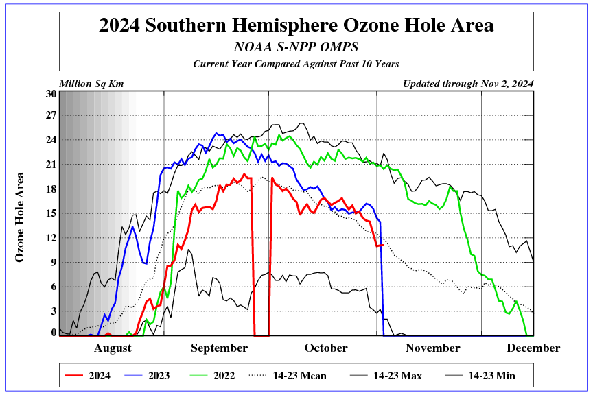
The SSW also driving down the size of this year’s Antarctic ‘ozone hole’, might smallest in 15 years, maybe smallest in 30 years…
https://ozonewatch.gsfc.nasa.gov/
The Ozone boys have been looking at what keeps the ozone hole going for many years.
With all the resources they have been given, I was hoping that an SSW of this magnitude would be forecast or the cause at least explained.
The ‘Ozone boys’ don’t seem to have commented recently on observations that a quiet sun increases ozone above 45 km contrary to previous expectations.
The consequence is that the increase in ozone above 45km feeds down from the mesosphere into the stratosphere over the poles within the descending polar stratospheric vortex (not the tropospheric circumpolar vortex).
The increased ozone absorbing incoming solar energy causes increased warmth at height and that supplements the background adiabatic compression warming that occurs during the descent.
Thus one sees more heat in the lower stratosphere than would have been the case with less ozone and it follows that SSW events become more frequent, more intense and longer lasting above both poles.
A warmer lower stratosphere over the poles pushes tropopause height downwards which forces cold polar surface air outwards and jet stream tracks become more meridional.
That increases global cloudiness which reduces solar energy into the oceans and in due course the system cools down.
It also follows that the more active sun of the late 20th century caused a reduction of ozone in the mesosphere which then caused the expansion of the ozone hole over the Antarctic and lower levels of ozone (but no actual hole) over the Arctic.
It was never anything to do with CFCs.
With the quiet sun we now see a reduction in the size of the Antarctic ozone hole.
http://joannenova.com.au/2015/01/is-the-sun-driving-ozone-and-changing-the-climate/
A warmer lower stratosphere over the poles pushes tropopause height downwards which forces cold polar surface air outwards
Leading to cold weather outbreaks in the SH:
https://www.iceagenow.info/chile-snow-surprises-inhabitants-of-la-araucania-in-full-spring/
Furthermore, the pressing down of the polar tropopause inevitably results in a lifting up of the equatorial tropopause.
Thus, to balance anomalous ozone induced adiabatic compression and heating above the tropopause over the poles we see anomalous adiabatic decompression and cooling below the tropopause in equatorial regions.
That appears to fit perfectly with Roy’s observations.
That internal system balancing process is what keeps atmospheres stable so that they can retain long term hydrostatic equilibrium rather than being lost to space or falling to the ground.
All potential destabilising influences, including the radiative characteristics of atmospheric gases are neutralised in a similar fashion otherwise atmospheres could not be retained.
Thank you Stephen that appears plausible, but I am sure others will point to AGW.
During SSW, ozone accumulates in excess in a certain area and the ozone stain slowly moves in the stratosphere. In this region, air is exchanged from the upper troposphere and the lower stratosphere.

Galactic radiation now reaches maximum values in cycle 24.
https://cosmicrays.oulu.fi/
Due to the two centers of the magnetic field in the northern hemisphere, the sudden warming of the stratosphere causes much stronger effects on the surface.
https://youtu.be/bminxfVGa5w
The surface temperature in medium latitudes decreases during SSW.

It should be interesting to see how large that ozone hole is this month.
This figure shows the progress of the size of the ozone hole in comparison to other years. For more information about this graph go to the ozone hole web page.
Roy, some questions.
How long will this phenomenon last, can we expect higher temps for 2 months and then a sudden drop once things reequilibrate.
Second if it continues to spike could it indicate a satellite algorithm problem?
DMI has some amazing dips a few years ago due to such problems.
Your figures showed a remarkable concurrence of NH, SH and tropic anomalies.
Is it a feature that NH and SH anomalies are expected to be different and is there any truth to the perception that when it is abnormally hot in the NH it is abnormally cold in the South?
Ta.
Not sure how relevant, Antarctic did began to show large zonal temperature anomaly variations in August.
https://imgur.com/a/sfperGf
The biggest change is rooftop solar panels – they must the cause..
Huge falsification of global temperatures is going on to conceal cooling since 2016.
http://clivebest.com/blog/?p=9142
http://clivebest.com/blog/wp-content/uploads/2019/09/Aug-2019.png
http://clivebest.com/blog/wp-content/uploads/2019/09/V4-monthly-adjustments.png