Guest post by AJ
Kriged Sea Level Rise

Introduction
This post shows a reconstruction of sea level rise (SLR) derived by kriging tide gauge data corrected for vertical land velocity. Kriging is a statistical interpolation method which takes into account how observations differ over distance. This method is employed widely in the mining industry to estimate the mineral concentrations of ore bodies. It has also been used to create global surface temperature reconstructions such as those produced by “Berkeley Earth” and “Cowtan and Way”.
Results
Here is the reconstruction from 1900 to 2017:

Figure 1. Kriged Sea Level Reconstruction 1990-2017. black: 1900 onward trend, red: 1960 onward trend.
The overall linear trend is 2.3 [2.2 to 2.4] mm/yr. The trend from 1960 onward is 2.5 [2.4 to 2.6] mm/yr. The linear trend since 1993 is 2.5 [2.3 to 2.7] mm/yr. This is significantly less than the 3.3 mm/yr trend estimated by satellite altimetry data. No significant acceleration or deceleration was found in either regression.
The 20th century SLR was about 23 cm. The predicted 21st century SLR is 22 cm and 26 cm using the 1900 and 1960 onward quadratic regressions respectively.
The reconstructed values are available here.
Methods
First the tide gauge observations were obtained from the Permanent Service for Mean Sea Level (PSMSL). Specifically, the Annual Revised Local Reference (RLR) dataset was used. Stations that were marked with a quality flag and yearly data that was flagged for attention were excluded.
The tide gauge stations were then matched up to the closest GPS stations listed on the vertical land velocity table from SONEL. The combined data was filtered so that only gauge stations with a GPS station within 80 km were retained.
The combined data was also filtered to exclude stations where the vertical velocity was outside the two standard deviation range (+/- 5 mm/yr) or if the associated uncertainty was more than 0.5 mm/yr. This was to exclude observations from what might be unstable ground. Here is a map of the remaining tide gauges:

Figure 2. Sampled Tide Gauge Stations
From the map we can see that the coverage is uneven. This unevenness is further exacerbated when we consider temporal coverage. When kriging, stations will not be of equal effective weight. Stations which do not share much overlapping range with others are more significant. For example, isolated stations in the Southern Ocean will be relative heavyweights compared to the lightweights in the densely packed North Atlantic.
The difference between consecutive years was then taken on the remaining observations and adjusted for vertical land velocity. This was then further filtered to only retain values that were within two standard deviations of each year’s mean. Using this data, the following variogram was generated:

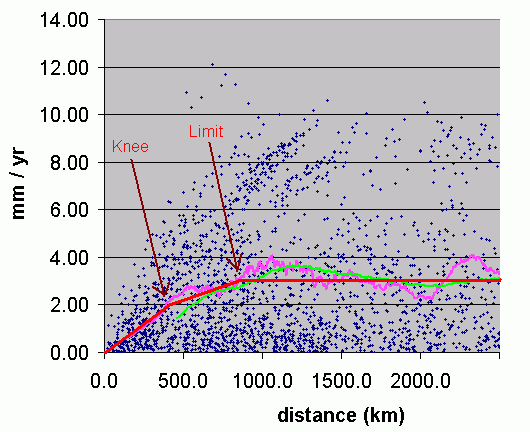
Figure 3. SLR Variogram. black: spherical fit, red: exponential fit
This variogram is actually an average of four recent years of observations (2013-2016). The spherical fit was subsequently used to krig the reconstruction. This shows that the observations between neighboring stations are highly correlated, with a y-intercept (nugget) of zero. The observations show a relative prediction skill out to a range of about 2150 km. The maximum distance for kriging was limited to this range.
One reason why the “GPS within 80 km” rule was chosen was that beyond this value the nugget crept above zero. A non-zero nugget indicates a measurement error in the observations.
Initially this post was going to use a variogram derived from Aviso satellite altimetry data. This idea was abandoned after the following variogram was generated, which again was an average of four recent years:

Figure 4. Aviso Pacific SLR Variogram. black: spherical fit, red: exponential fit
The relatively high nugget value suggests a large measurement error in the observations. Maybe this is due to the wavy roughness of the ocean surface? Perhaps the shear number of observations cancels out this noise? It is noted that an exponential fit works best with this dataset.
The Aviso data was used to compute a 5×5 degree grid of ocean coordinates. This was a lower resolution version of the 0.25 degree grid provided. This is the result:

Figure 5. 5×5 Ocean Grid
This grid looks entirely suitable for kriging. There are a couple of anomalies (Caspian Sea, North Pole), but nothing that would materially impact the results.
Kriging was then performed using the filtered observations, spherical fit, and grid. In addition to the reconstruction displayed at the top of this post, the number of observations for each year and the percentage of the Earth’s oceans kriged was also tallied:

Figure 6. Number of observations per year

Figure 7. Percentage of oceans kriged
It is noted that the number of observations follows a smoother trend than the percentage of oceans kriged. This is an indication of the impact of heavyweight stations as observations become available or unavailable. Additionally, the small sample sizes in the early portion of the time frame explains the associated noise in the reconstruction.
Conclusion
This post calls into question the narrative that SLR is accelerating. It demonstrates that it is possible to create a linear timeline by employing a suitable method and making reasonable parameter choices. This may also explain why many tide gauges do not show acceleration.
Of course there were many arbitrary choices made in this analysis, so confirmation bias is a concern. Due to the various filters, only about a quarter of the PSMSL observations were used, mostly because a suitable match to a GPS station was not found.
One example of how a choice can impact the results is shown by what value is given to the maximum distance parameter used for kriging. This reconstruction used the range taken from the variogram fit (~2150 km) as this was considered the maximum predictive distance that an observation had relative to other observations. By varying this parameter one can see how this impacts the predicted 21st century SLR:

Figure 8. Predicted 21st Century SLR based on 1960 onward regressions given different values of maxdist parameter used in krige() function.
This shows the predictive sensitivity to this parameter’s value and brings up the question of what value is most appropriate. This post will not examine that question. It is simply noted that parameter choices can significantly impact the results. This is probably a factor in any tide gauge SLR reconstruction.
Thank-you for your time.
Links
The R source code and Intermediary files can be found here
Report this ad
References
- Permanent Service for Mean Sea Level (PSMSL), 2019, “Tide Gauge Data”, Retrieved 01 Apr 2019 from http://www.psmsl.org/data/obtaining/.
Simon J. Holgate, Andrew Matthews, Philip L. Woodworth, Lesley J. Rickards, Mark E. Tamisiea, Elizabeth Bradshaw, Peter R. Foden, Kathleen M. Gordon, Svetlana Jevrejeva, and Jeff Pugh (2013) New Data Systems and Products at the Permanent Service for Mean Sea Level. Journal of Coastal Research: Volume 29, Issue 3: pp. 493 – 504. doi:10.2112/JCOASTRES-D-12-00175.1. - SONEL: Santamaría-Gómez A., M. Gravelle, S. Dangendorf, M. Marcos, G. Spada, G. Wöppelmann (2017). Uncertainty of the 20th century sea-level rise due to vertical land motion errors. Earth and Planetary Science Letters, 473, 24-32.
- Aviso: The altimeter products were produced by Ssalto/Duacs and distributed by Aviso+, with support from Cnes (https://www.aviso.altimetry.fr).
Great analysis, and a superb WUWT contribution. No acceleration. Plus the krigged estimate closes (see my guest post SLR, Acceleration, and Closure). Also shows yet again that the satellite altimetry stuff is erroneous, and not fit for purpose.
“Also shows yet again that the satellite altimetry stuff is erroneous, and not fit for purpose.”
No, it doesn’t. Firstly, the difference isn’t actually that much. And what there is can easily be attributed to the different regions of measurement. The % of oceans kriged never gets more than about 70%. That of course is not the only reason why there might be a discrepancy, but it is a sufficient one.
Another worth noting is in an observation near the end:
“It is simply noted that parameter choices can significantly impact the results. This is probably a factor in any tide gauge SLR reconstruction.”
Fig 8 makes the point.
“…Firstly, the difference isn’t actually that much…”
Well SLR “isn’t actually that much” to begin with. But relatively, speaking, 3.3 vs 2.5 seems substantial. The linear trends were stated to be significantly different.
“… And what there is can easily be attributed to the different regions of measurement…”
No, you mean that the discrepancy can possibly be attributed to that. You have no evidence at all to claim that the difference in trends can be attributed to that, let alone “easily.”
“…That of course is not the only reason why there might be a discrepancy, but it is a sufficient one…”
It isn’t that there “might be a discrepancy”…there IS one. And it is a sufficient reason how? It “may” or “might” be sufficient, but to claim that it “is” without any supporting evidence is farcical.
The author was very soft about his conclusions (“this post calls into question the narrative that SLR is accelerating”) and raises the issues of potential confirmation bias, parameter selection, etc. If only others were so open and honest.
Yes, I applaud the author’s clarity about the impact of the choices made. This is how scientific analysis should be done. The difference between 2.5 and 3.5 is large proportionally but 25 or 35 cm / century it not a problem either way.
The sensitivity of the quadratic model to choice of maxdist highlights the fact that this is extrapolation well outside the reference data period.
The Guardian would surely report this as: ” New study shows sea levels may rise by as much as 50cm by 2100″.
When I got as far as reading figure 3 , I thought that I would have stopped at about 1500km and could not see why he chose to use 2100. It seems the quadratic would be showing some curvature ( acceleration ) if a shorter distance was used. Though 35cm, just over a foot is not a problem anyway.
This idea of “nugget” as an indication of data reliability is very interesting. I stopped taking satellite altimetry seriously about 10y ago due to the blatantly political and non scientific attitude of those responsible for extracting and presenting the data.
It is not roughness which is the problem, that probably would average out. It is that the strongest reflection is from the bottom of the swell, so they need to try to estimate the height of the swell from the noise. This involves modelling and parameter choices. Sadly they are a lot less open about the effect of such choice than the present author.
There is also the question of how graft the various satellite datasets together. That also involves subjective choices and is a factor in the long term trend of the ensemble. Finally, don’t forget 0.3mm/y GAIA adjustment for hypothetical deepening of the oceans. This means they are communicating a false sea level, ever higher above the waves each year. So 3.5 is nearer to 3mm in REAL sea level.
Greg, what would be wrong with using the height of the troughs of the swell if they give the best reflection? They would eliminate messing with froth tops of waves. They are ‘waves’ after all.
Gary Pearse wrote, “what would be wrong with using the height of the troughs of the swell if they give the best reflection?”
The problem is that during a flat-calm the measured sea-level would be much higher than during windy conditions. It would create an appearance of very large sea-level change from mere changes in weather.
What’s more, those fake sea-level changes would be a couple of orders of magnitude greater than the actual sea-level changes that you’re trying to detect.
In addition to Dave Burtan’s comment regarding: “what would be wrong with using the height of the troughs of the swell if they give the best reflection?”
If indeed, global wind velocities on average decrease due to a reduced temperature differential between the polls and mid latitudes (as is predicted), there would be a false sea level rise indicated by reduced wave heights.
Excellent reply!
No SL calculations from Tide Gauges that are not corrected by Continuous GPS on Same Structure — that means mounted on the same pier or sea wall — are not valid for any purpose other than Local Relative Sea Level.
Using CGPS from distant locations may help to inform us of continental movements. But most movement at tide gauges is from subsidence of the structure to which the gauge is attached.
The technical application is CGPS@TG-SS. We know from satellite ea level data that the seas are not uniformly rising not flat but bumpy, and that some locations are rising and some going down. Thus kegging is inappropriate for determining ea level or its trend overtime.
“But most movement at tide gauges is from subsidence of the structure to which the gauge is attached.”
Surely if this was a uniform issue then subsidence of the structures would mean tide gauges should have on average greater than actual SLR signal?
pbweather ==> Yes, that’s the point. However, some structures with tide gauges attached actually rise (get further from the center of the earth) as they do in much of Alaska.
The CGPS must be attached to the same structure as the Tide Gauge to get any data on how the sea surface is differing — rising or falling. One must have several (at least three) years of CGPS data for any reasonable guess-timate of vertical movement of the structure.
The analysis above uses CGPS stations as much as 80 km away from the tide gauge — which is just silly — it is only done because that’s the only data they have — they know it is not really valid except cor gross movements of continental masses.
Liquids aren’t bumpy. They can be in motion, but water is always falling to the lowest point, it cannot raise in bumps. That illusion is from the land moving rather than the ocean. Krigging seems like it works just fine here, since it was conceived to deal with rising and falling land features.
Ged ==> I am afraid that simply is not true for the oceans.
See Jason-3 results for sea levels around the globe.
The sea (seas) is not a bathtub.
Another data point: Sea level rise rate *according to tide gauges* was .76 mm/year greater in 1993-2013 than the 1.5 mm/year recorded in 1972-1992. This .76 mm/year acceleration of sea level rise from one 21-year period to the next was presented as opposing a much greater acceleration of sea level rise indicated by the Church & White dataset that happened when satellites started producing data that was considered by Church & White. This is according to a WUWT article whose author also said “And this makes it very likely that Church and White are manufacturing sea level acceleration where none exists”, after that author derived .76 mm/year of acceleration of sea level rise to present in opposition to the 2.1 mm/year acceleration that depends on a satellite record that started with 1993.
https://wattsupwiththat.com/2018/12/17/inside-the-acceleration-factory/
Mr Stokes, if the UK environmental agency is extrapolating satellite data/alarmist scientist advice, to predict 40″ of sea level rise by 2100 when all available tide gauges suggest less than 6″, and then using that to cost justify £multi-million schemes, I’d say that was quite important, wouldn’t you?
Nick,
70% is enough to have a difference between the two trends but my understanding is that the satellite data doesn’t agree with tide gauge… well anywhere really. I’m 99% sure those still invested in the AGW world have checked and would have loudly proclaimed that satellites do match tide gauges and deep sea isn’t being represented well in tide gauge data. In fact we should have heard it from the tops of the towers- sea level rise worse than we thought — or some such rubbish. Is that something I missed in the pseudo-literature?
I’m curious why you believe actual measurements are inferior to an interpolation? Not defending the satellite measurements being better as I’ve always been skeptical how they could measure such small increments with the claimed accuracy.
The waviness of the oceans gets modelled. It would be good to check if there is an SST input.
“I’m curious why you believe actual measurements are inferior to an interpolation?”
I’m curious why you call satellite altimetry actual measurements. Tide gauges are actual measurements and have simple mechanical damping techniques to average out the waves.
Bouncing E-M radiation off the trough of the swell and trying to calculate the average of where still water would be is the usual climatological exercise of tweaking you guesses until it matches your expectations of a reasonable value, or a politically expedient one to further your “cause” of saving the planet.
+1
The bigger problem is none of the historical sea rise measurements are playing out on Jason 3.
The moment it went live everything flatlined because it deals with sea level differently. Even if you look at recent University of Colorado Boulder publications claiming acceleration
https://cires.colorado.edu/council-fellows/r-steven-nerem
See that big flatline at end that is Jason 3 …. 3 years almost dead flat and counting.
When it gets to about 10 years I guess they will have to start talking about it but more than likely they will do a Jason 3 adjustment.
LdB, that Jason 3 “flatline” seems to have ended:

Source:
https://www.aviso.altimetry.fr/en/data/products/ocean-indicators-products/mean-sea-level/products-images.html
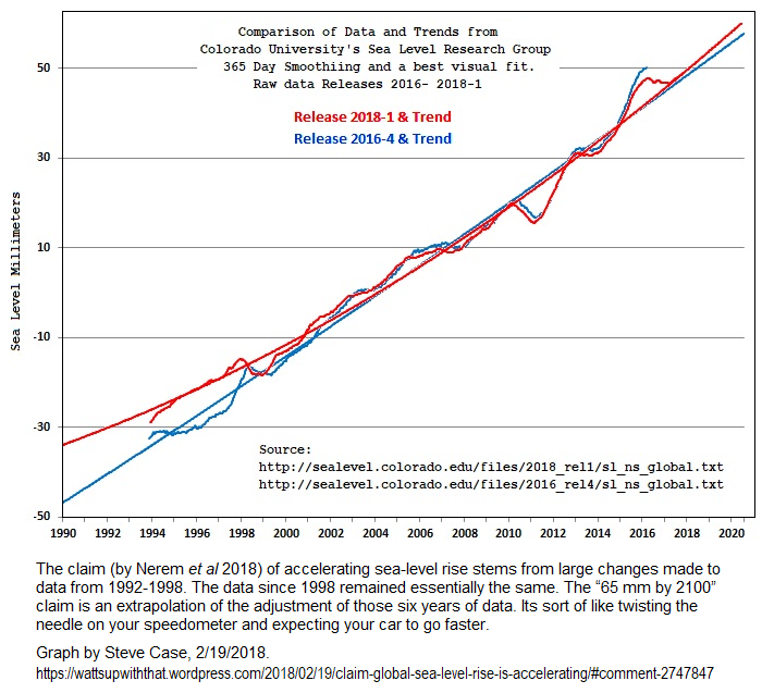
As for Nerem, the reason his 2018 graph shows apparent acceleration (the upward-curvature) is that he created that acceleration through adjustments to 20 year-old data!
Specifically, he slowed the rate of rise of sea-level rise “measured” by Topex-Poseidon prior to 1998, thereby creating the appearance of acceleration when the early Topex-Poseidon data is compared against the newer satellites’ data. This graph by Steve Case shows what Nerem did:
Thanks Rud! I believe the approach is valid. Hopefully I haven’t flubbed the execution. I was surprised that I couldn’t find any studies using this method. Kriging seems to be a fairly standard method for addressing spatially inhomogeneous data. Maybe this is fruit for the picking by an actual scientist.
I’m grateful that WUWT published this. Hopefully it gets a good going over. All criticisms are welcome.
“Hopefully I haven’t flubbed the execution. I was surprised that I couldn’t find any studies using this method.”
It looks well executed to me. But the weakness is still the sparsity of the data, which is probably why it hasn’t been done elsewhere. It’s rather like the original Hansen&Lebedeff, 1987, where they didn’t have SST data but essayed a global average temperature anomaly by extrapolating coastal readings over the ocean. It upweights islands especially, as here. But they had a lot more data than SLR offers.
You didn’t say exactly how you integrated the interpolated result. I hope you used cos latitude weighting. But there are better grids (than lat/lon) you can use, for example cubed sphere or icosahedron.
Yes I used cos latitude weighting.
About the maxdist parameter, if I had just used a straight average of gauges without interpolation, my predicted 21st century SLR would be in the neighbourhood of 80cm. You can see this in figure 8 where the highest values accompany the lowest maxdist choice. I think this is also a factor in the higher maxdist values as the previously unkriged grid points will get the average of what should be equally weighted stations.
Did I miss it, or is a substantial part of the discrepancy just the 0.3 mm per year that is manually added to the satellite rate to account for ‘increasing ocean basin volume’ due to continuing isostatic rebound? 2.5 mm per year from tide gauges versus 3.0 mm per year from satellites (against a geographically stable shoreline) doesn’t seem to me a very big difference.
Yes… the proper comparison is 3.0 vs 2.5. Not especially large considering the uncertainties.
Nick , there is an obvious way in which extrapolating coastal temperatures out across the ocean would bias SST. It is possible that water could “pile up” around islands to produce a similar bias in tide gauges?
Greg,
It isn’t just islands. Whenever you have an open-sea oscillation, wave or tide, which has been damped, then the damped mean is very likely to be different from the linear mean. Tide gauges are likely to be in such situations, in ports etc. I was once marginally involved in a paper referring to this effect in groundwater (example b, p 517).
There will be a bias, but the question is whether it varies over time.
Even before I got to the end, I was thinking ‘Torturing the Data’.
raw tide guage data must be adjusted for isostatic land height changes. The advent of dGPS and deployment of measurinf stations now offers a rational and precise method for making such corrections. In making such corrections some choices have to made. Those choices, properly explained, are foundational in observational applied sciences.
So not torturing.
Torturing data in climate related studies usually involves PCA type analyse that Mann and the paleoclimate reconstructionists infamously use on treemometer data to create hockey sticks.
Satellite sea level is adjusted for GIA with 0.3mm/y because the seabed is sinking and they want to show the amount of water in the oceans.
If the seabed sinks 0.3mm/y then the land must rise 0.6mm/y to keep the Earth volume the same.
In that way the Holgate-9 SLR that has 2mm/y rise is indeed very close to the satellite sea level.
There are a number of arbitrarily chosen parameters, so the whole “wiggling the elephant’s trunk” thing is a concern. Because remote gauges will heavily outweigh others, I’ve implemented a number of quality filters so that erroneous data doesn’t skew the results.
Many specialist ore reserve scientists from the mineral industries are thoroughly familiar with kriging, especially its advantage of validation after mining. Any such specialists reading the post should contribute comments, because there is uncertainty about the origins technique in the wider community.
My colleagues in the 1970s were world leaders in geostatistics and they produced valuable ore estimates way back then that were shown post-mining to reconcile for grade and tonnes to better than 10% for their first major mine. Geoff
Far from an expert but this seems to be similar to using results from only areas high in chalcocite to figure out the copper content of an ore body that is mostly chalcopyrite. Its a big assumption that tidal guages are a good reflection of what is happening in the deep ocean to within mm.
Apologises for not being able to remember the pacific island but one was on the news because a linear fit to its tidal measurements showed it would be swamped soon (because of climate change). The measurements started a few years before the El Nino that had dropped the local sea level something like half a metre for the year. You would really need to know how big the difference was between the inshore readings and the general area in deeper oceans because of changes in currents, rather than assume correcting for subsidence etc. is enough.
This is an interesting approach and corroborates other analyses showing no sea level rise acceleration. Thanks for posting your hard work!
The period from 1960 onwards coincides with the rising phase of the ~60 year cycle, which peaked around 2005.
Sea level rise accelerates during this phase of the cycle and decelerates during the downwards phase.
The Battery in NY has a long dataset which shows the cycle. It matches the AMO rather well.
I weep when one uses satellites to invalidate NY Battery actual SLR measurements. Going from cm measurements to mm accuracy boggles this scientific/mathematics mind.
I hope all of the CliSci scientific fraud is eventually documented. History, however, is written by the victors. Truth and history is whatever your masters say it is.
“Statistical interpolation” sounds like more modeling to me although I like the results 🙂
In general, isn’t interpolation less risky than extrapolation?
“This method is employed widely in the mining industry to estimate the mineral concentrations of ore bodies. It has also been used to create global surface temperature reconstructions . . .”
Note that Kriging has been commonly used to prepare isocon (isoconcentration) maps of groundwater contamination from groundwater analytical data.
I’m curious about how well the tide gauge data match with the Aviso cells that overlap them. In other words is there an overall bias between the satellites and tide gauges (i.e. ground truth) or is the bias geographically dependent?
I doubt they match up very well. Neighbouring Aviso cells don’t even match up with themselves. The values should be highly correlated, but they are not.
Bear, I agree with AJ.
What’s more, the satellites cannot measure sea-level anywhere near land. In fact, even the passage of a ship can mangle their measurements.
Physicist Willie Soon explains many of the problems starting at 17:37 in this very informative hour-long lecture:
Is kriging appropriate for sea level? After all, it is fundamentally true that water seeks its own level while land is pushed willy nilly by many forces.
There is nothing to verify the new satellite sea surface level altimeter data…EXCEPT THESE (and other properly) KRIGED TIDAL DATA SETS.
What are they going to do…compare satellite sea level altimetry against models??
The satalllire data is showing a slight acceleration that is seen in FEW OF THE TIDAL GAUGE RECORDS. That is a fail.
Satellite sea level altimetry may someday become the “gold standard” but there is a lot more work to do to make that happen.
How are they getting away with all of these CAGW lies? Has every scientist in the field sold out??
” … so confirmation bias is a concern …”
Looks like 2 stations shown for Queensland Oz. Cape Ferguson is there, possibly Rosslyn Bay? The 2 stations operated by BoM (Bureau of Meteorology), famous for “adjustments”. There are another 42 permanent tide gauges in Queensland that are not operated by BoM. Rosslyn Bay actually has two tide gauges in the same tide race that show different results, which seems a bit unlikely. The rest all show different results, but none are necessarily wrong or manipulated.
The problem with SLR is that 65% of the gauges show little change. 10% show that sea levels are decreasing. The remaining 25% show sea levels increasing. An average of all this data will show a slight increase in sea levels. If you took a medium value then there would be negligible rise. An average value shows a modest increase (around the 1.7mm/yr). With that data how could you make any certainty about what is actually happening.
You only need one tide gauge….if it’s one of the oldest…and out on a rock in the ocean….covered in military…that depends on the accuracy of GPS for everything they do…and the military says it ain’t movin
https://tidesandcurrents.noaa.gov/sltrends/sltrends_station.shtml?id=8724580
Fort Denison says less than 1mm/year
https://tidesandcurrents.noaa.gov/sltrends/sltrends_global_station.shtml?stnid=680-140
Uh, your citation of the RSL information at Key West, FL is supposed to tell us anything about global sea level rise? The ground is sinking, FCS!
Holy Grig Batman, does this mean we are going all to drown next year instead of this year ? Woohoo, the Maple Leafs get one more chance at the Cup !
How do you even determine a reference point, on a viscous blob running thru multiple “gravity” fields ?
There must be a limit to any accuracy, no matter the precision of the measurements.
If you take the trouble of downloading all the PSMSL tide gauge data and then calculate the acceleration since 1993 to compare it to Colorado University Sea Level Research Group’s value of 0.084 mm/yr² you will find out that the range of acceleration in the 208 PSMSL stations that report 100% for that time series is on the order of -0.5 to 2.6 mm/yr² Attempting to tease out a mean or median accurate to 4 places which is what would be required is a fool’s mission.
“This is significantly less than the 3.3 mm/yr trend estimated by satellite altimetry data. …”
Part of the reason for that might be that although satellites measure and report relative sea level change — what you’d observe on your backyard tide gauge — the numbers are then fudged upwards by applying a roughly 12% correction for hypothetical glacial isostasy. There are reasons for that (not good ones IMHO). Anyway the number you should be checking against for satellite estimates is probably closer to 2.9 mm/yr than 3.3mm/yr.
I’d note that reliably detecting a SMALL acceleration in sea level rise probably needs many decades worth of very good data. I don’t think we have that.
I have some reservations about applying kriging to sea level estimates is a good idea and also about assuming GPS measurements made many km away are valid for tide gauges whose elevation changes may be highly local. (Best to nail a GPS to the gauge and hope no one steals it I think). OTOH, it’s not like the alternatives to kriging are all that stellar.
Anyway, thanks for the effort.
” the numbers are then fudged upwards”
AVISO describes its process here. They don’t perform a GIA on local values, which I think are what AJ is using. GIA is appropriate if you want to use sea level as a measure of ocean volume, and they apply it to their global values.
I’ll make that elephant wag its trunk, too.
GIA is appropriate if you want to use sea level as a measure of ocean volume
Then their graph should be labeled “Ocean Volume”
“GIA is appropriate if you want to use sea level as a measure of ocean volume”
That’s correct Nick. Conceptually at least, one needs to correct for ongoing distortion of ocean basins if one ever hopes to get closure over the sum of SLR minus ocean thermal expansion, ice melt, new reservoir storage, aquifer uptake and downdraw. However the seventeen people in the world who want/need that correction are perfectly capable of making it on their own. And they probably want to do it their own way anyway. It’s not like GIA values for mid-ocean locations are anything other than a moderately wild guess.
“They don’t perform a GIA on local values, which I think are what AJ is using.”
I think you’re correct that local GIA corrections aren’t made to individual satellite measurements — just a global adjustment to the final SLR number. However, my reading of the post is that the AVISO satellite data was only used to try to figure out an appropriate maximum distance parameter for kriging. I don’t think that they used the AVISO data to recompute satellite SLR values. But if they did, I think that the number they’d want to compare to tidal gauge measurements would be relative (satellite observed) SLR without an isostasy correction.
It’s confusing. But “GIA adjustments” for satellite observed SLR do something different than GIA for individual tide gauges.
I used Aviso’s monthly 0.25 degree gridded data. The GIA is not applied to it. Aviso was not used in this reconstruction except to create my ocean grid to krig to. The variogram was for information purposes only. I was actually able to reproduce Aviso’s SLR timeseries almost exactly. What little difference there was I attributed to me excluding incomplete grid points which were mostly in the high latitudes. Ice I think.
The overall sausage making that goes into estimating mean sea level any any point from instantaneous reflections and making a long term satellite record from the different platforms means we will never have that.
The real problem is in extrapolating that far outside the data, especially using a quadratic.
Don K wrote, “the numbers are then fudged upwards [by AVISO] by applying a roughly 12% correction for hypothetical glacial isostasy.”
They are actually adding a flat 0.3 mm/yr GIA fudge factor, as an estimate of the effect of the presumed ongoing sinking of the ocean floor, in isostatic response to the last deglaciation.
AVISO used to make that GIA adjustment optional in their graphs, but they removed that feature. I wrote to them and asked them to restore the feature. They politely refused.
Yes, I had a similar exchange with the Boulder group years ago. They apply an inverse barometer adjustment and the unadjusted data disappeared from public view. I wanted to see the difference since I can’t see how I.B can affect global means. The “community” clearly has an agenda to communicate.
Despite that, both groups clearly label their data as being Mean Sea Level not an “index” or “indicator” of oceanic volume, which is misleading since the primary implication of sea level rise is its effect on coastal populations and this is what they are trying to scare everyone with.
I can only assume they adopt a similar attitude when selecting the parameters of the models used to extract average sea level from a signal measuring the trough of the swell.
” I wanted to see the difference since I can’t see how I.B can affect global means.”
Long term it possibly doesn’t. Shorter term, I think that the distribution of high and low pressure isn’t random. My guess is that average air pressures might be a bit higher on average over landmasses than over water. Especially in Summer and early Autumn. But that’s just a guess. A meteorologist might know.
“I can only assume they adopt a similar attitude when selecting the parameters of the models used to extract average sea level from a signal measuring the trough of the swell. ”
I read somewhere in an obscure pdf that what they do is point a radar “down” at the Earth where the pulse has a footprint of 10km or so. Somewhere (probably) near the middle of the footprint the pulse will start to strike the tops of the highest waves and reflect. As time passes, the pulses reflect lower on the waves in the middle of the footprint and on the crests further out. To further complicate things, more energy is reflected back to the radar from troughs than the crests. Anyway, what the receiver at the satellite sees is a rising waveform of reflected energy. They pick the midpoint of the rise. That represents the “measured” sea level.
Dave. You’re correct about GIA and I agree with you. It’s nebulous at best and has traditionally been used as a cosmetic “correction” to get around the fact that we rarely have a good estimate of the ongoing tectonic changes in tidal gauge “elevation”. It’s a sort of “a dubious correction is probably better on average than no correction at all” thing.
However, there is a valid justification for correcting observed (“relative”) sea level changes for changes in ocean volume. If one doesn’t do that, one can’t (in concept) sum up sea level rise, ocean thermal expansion, ice volume changes, water storage, aquifer downdraw, etc,etc,etc with appropriate signs and come up with zero. I don’t think we’re supposed to worry our pretty little heads about the fact that we are many decades or centuries from being able to do that even if we actually knew what the changes to ocean basin volume are. Which we don’t.
Footnote: Aviso told me, “We do include the corresponding uncertainties in our total uncertainty assessment of 0.5 mm/yr (PGR participates by 0.05mm/yr at 90% CL).”
But to the best of my knowledge Prof. Peltier and his colleagues have not published uncertainty estimates for their 0.3 mm/yr ocean basin GIA estimate, nor for any of their other GIA / PGR figures. Tamisiea, 2011 gives a much broader range: 0.15 to 0.5 mm/year.
I wonder whether Aviso just assumed they could approximate Peltier’s uncertainty by using half of his last (only!) significant digit?
AJ = Andre Journel?
(Stanford Professor of Geostatisics, who “wrote the book” on Geostatistics)
No. Just a random guy with a computer and some data. Maybe qualified to write at WUWT post, but that’s about it.
I am quite curious about the cause of the fairly substantial variations around the mean, especially in the first half of the 20th century. Don’t seem to correlate with the known warmer periods. Any thoughts?
Lower number of obsevations leading to greater variability perhaps?
Is the K silent?
I was lead to believe that the Hong Kong Harbour gauge was a significant part of this global network, but it’s not shown here. Nothing at all in the South China Sea nor around the sub continent of India.
It’s good to see spatial statistics applied to tide gauge data, as the gauges are unevenly distributed for several reasons. One long-standing reason is that they tend to be sited and maintained in operation where people are most concerned with changes in sea level. Some long-standing gauges in Scandinavia were established because harbors were becoming hazardous due to post-glacial rebound of the land. A few of these gauges appear to be in the present compilation, but other gauges in almost all the Arctic and all the Antarctic are ignored. A quick look at the records for gauges such as Churchill and Argentine Islands shows that the “global” rise would be much less if these vast regions were represented.
Since people install and maintain gauges, they tend to be where populations are largest, that is where porous sediments provide abundant groundwater and hydrocarbons. Extraction of these fluids has caused land subsidence under many of the gauges in the compilation.
Perhaps my GPS filters were too restrictive. I chose a velocity range of +/- 5 mm/yr and uncertainty limit of 0.5 mm/yr. I believe there is a need for filtering though. You can see the SONEL’s tide gauge / GPS pairings in the link below. Check out the station on the coast of Chile. It’s showing a SLR of 31 mm/yr. Looks erroneous.
https://www.sonel.org/-Sea-level-trends-.html?lang=en
I agree, AJ, that’s definitely wrong.
Hover your mouse cursor over it and you’ll see that it’s Antofagasta, Chile, PSMSL station no. 510.
The mean sea level (MSL) trend at Antofagasta, Chile (calculated by my sealevel.info site) is -0.87 ±0.39 mm/year, based on monthly mean sea level data from 1945/12 to 2016/12. I.e., sea-level is falling there. Here’s a graph:
http://www.sealevel.info/MSL_graph.php?id=510
Here’s NOAA’s graph and trend analysis for Antofagasta; they calculate an almost identical trend of -0.87 ±0.38 mm/year:
https://tidesandcurrents.noaa.gov/sltrends/sltrends_station.shtml?id=850-012
When I last looked at the GPS-measured vertical land motion data, a few years ago, it seemed to be extremely rough. I concluded that it was not fit for purpose: the GPS satellite system just isn’t good enough at measuring altitude to get trustworthy measurements of vertical land motion.
The huge rate of sea-level rise reported by Sonel for Antofagasta there comes from subtracting their GPS-measured vertical land motion of 31.78 ± 0.33 mm/year from the sea-level measurements. But take a look at their graph of GPS measurements:
https://www.sonel.org/spip.php?page=gps&idStation=2608
Their GPS measurements of VLM span only 8½ years, and a third of that is gaps in the data, and the measurement period includes a magnitude 7.7 earthquake.
Another way of getting estimates of VLM is from Peltier’s model-based estimates:
http://sealevel.info/Peltier/
Peltier’s VM5a model output shows just -0.21 mm/yr (i.e., the land rising 0.21 mm/yr) for Antofagasta, Chile. His older VM2 model output shows -0.26 mm/yr (hardly different).
All sources agree that Antofagasta, Chile is experiencing uplift. But there the agreement ends. Based on the measured rate of sea-level rise, we can say with high confidence that the actual vertical land motion there is 2.4 ±0.6 mm/yr. That means Peltier’s model-based estimate is an order of magnitude too low, and Sonel’s GPS-based estimate (despite its claimed “±0.33 mm/year” precision) is an order of magnitude (nearly 30 mm/yr) too high!
If the GPS-measured VLM figures are that far off for Antofagasta, how can they be trusted for anywhere else?
According the global trends table at NOAA, 2.3 mm/yr is the 70th percentile. The median (n=368) is 1.5 mm/yr . The mode is between 1.3 and 1.8. So, 2.3 seems a bit on the high side. You would be hard pressed to push me over 2.0 mm/yr .
There is a reason the climate scientists have stopped talking about sea level rise …. it’s called Jason 3
Ask someone like Nick to show the Jason 3 data and then explain it.
That seems to be no longer true:

Source:
https://www.aviso.altimetry.fr/en/data/products/ocean-indicators-products/mean-sea-level/products-images.html
I’m not sure about the validity of this method because the resulting rate of increase is still too large.
The sea level rise in the North Sea over the last 150 years is very precisely known. The Dutch have a
rather pressing reason for accurate information. The rise is 1.9 mm/yr throughout the period, no acceleration at all. In fact we known that the whole river delta, on which much of the Netherlands finds itself, is sinking by 0.3 mm/yr. Its called a geosyncline, caused by the weight of sediments from the Alps dumped on it over thousands of years. That makes the true sea level change 1.6mm/yr.
The North Sea is in open contact with the North Atlantic. Archimedes, two thousand years ago, would tell you that therefore the sea level rise in the North Atlantic, and by extension, the rest of the oceans, is also 1.6mm/yr, apart from a tiny correction because the geodetic surface is not an exact sphere. The often mentioned local effects of currents and other effects are a red herring because they are more or less the same before and after any sea level rise.
Also, the Caspian Sea is a land-locked sea, not in contact with the oceans. Any measures there have no bearing on global sea level estimates.
Kriging is a component of geostatistics, a mathematical approach to understanding spatial measurements that is rather different to older correlation approaches and so a valuable adjunct.
As soon as one starts into kriging, often by construction of a semivariogram, one meets a need for subjective decisions, such as which method of curve fitting should be used to bring out a clear picture of the range, the distance beyond which prediction of more distant values fails, or the nugget, as the author has explained.
Success with kriging depends greatly on operator experience. The author here, AJ, seems to me to express experience, though I have already called for less rusty geostaticians to offer a better opinion. Geoff
I’m a geostatistical novice. My understanding is very high level. I’d be very interested to hear what a learned practitioner has to say.
Nice work, AJ!
Note: AJ, if you don’t read the whole comment, please do read the last paragraph, which is a question for you. (BTW, my contact info is on my sealevel.info web site.)
I smiled when I read about why you decided to use coastal (tide-gauge) data rather than satellite altimetry: you discovered yet more evidence that the satellite altimetry measurements of sea-level are of much lower quality than the best coastal (tide-gauge) measurements.
A decade ago, when I was new to this field, I did something somewhat similar. I’d never heard if Kriging, but I used the 159 stations in the GLOSS-LTT (LTT = “long term trend”) tide gauge set, and I weighted them according to their distance from other gauges, to calculate a global average rate of sea-level rise.
That is, I used NOAA’s numbers for the long-term trends at each site, but when calculating the average I deweighted tide gauges which were too close to other tide gauges to be considered fully independent, much as you did.
To do that properly, we must first know something about the granularity of the physical mechanisms (such as postglacial crustal rebound) which cause long term sea-level trends to vary between locations. In other words, how near must two tide stations be to each other for their sea-level trends to be more closely correlated than are the sea-level trends measured at stations which are widely separated?
To answer that question, I calculated two numbers for every pairing of tide stations. There were (159×158)/2 = 12,561 pairs. For each pair, I calculated the distance between the two stations, and the difference between their NOAA-calculated long-term sea-level trends. Then I graphed them, with distance on the X-axis and difference between sea-level trends on the Y-axis. The result is here:
https://sealevel.info/climate/MSLtrend_v_distance.htm
From the graph we can see that only at distances less than about 800 km is there any increase in correlation at all, and only at distances less than 400 km is there a substantial increase in correlation between sea-level trends measured at pairs of tide stations. Here’s the same graph, but limited to station pairs which are less than 2500 km apart:
https://sealevel.info/climate/MSLtrend_v_distance_to_2500km.htm
That’s a lot shorter distance than the 2150 km you used.
(The very different “range” numbers that we found could be because I compared similarity of long term trends, and you used similarity of short term trends. Since long-term trend differences are often caused by different things than short-term trend differences it doesn’t surprise me that the two approaches would find different ranges.)
Then I wrote code (in Perl) to appropriately weight each of the GLOSS-LTT sea-level trends, based on a piecewise approximation of that curve; here’s a graph showing the piecewise approximation:
The result I got was a distance-weighted global average sea-level trend of +1.133 ± 0.113 mm/yr.
However, that was ten years ago, and I am now aware of an error that I made. You see, some of the longest sea-level measurement records include an detectable acceleration in the rate of local sea-level rise, generally sometime between the mid-1800s and about 1930.
The most striking example is PSMSL gauge number 1, Brest, France. Brest is an important tide gauge, because it has measurements starting in 1807, spanning over two centuries!
The sea-level trend at Brest was 0.0 mm/year in the 1800s. But the sea-level trend there has averaged 1.5 mm/year since 1900. Here’s a pair of graphs which show the difference:
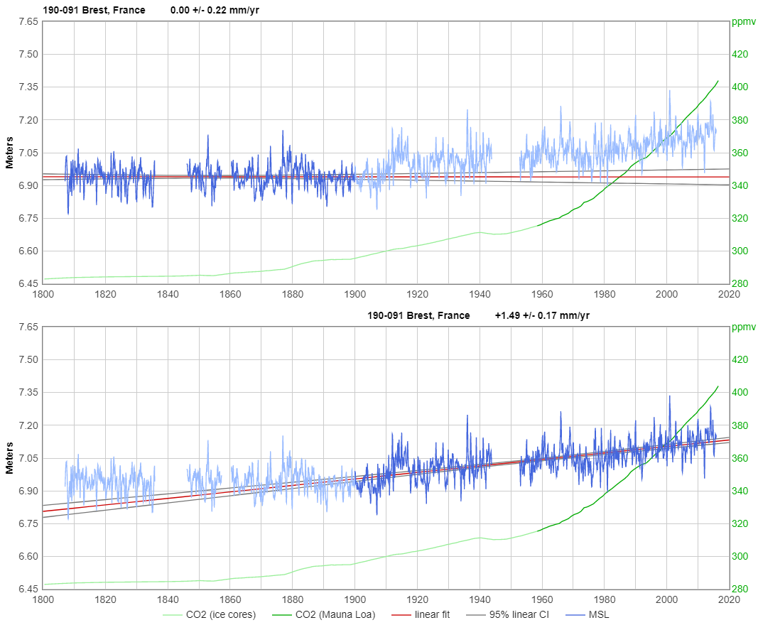
Since NOAA uses the entire period for their linear regressions, NOAA found a long term trend that was too low — and that was what I used for my calculations, ten years ago. That undoubtedly resulted in a slight underestimate of the globally averaged long-term trend.
I had intended to turn that work into a paper, but never got a round tuit. However, the details of what I did, and all the code, are here:
https://sealevel.info/climate/global_msl_trend_analysis.html#bydistance
More recently I used a different approach to calculate a “global average” rate of coastal sea-level rise, and I found it to be just under 1.5 mm/year:
https://sealevel.info/avgslr.html
AJ, how much of the 2.3 to 2.5 mm/year global average trend that you calculated was due to the GPS-based vertical land motion estimates that you used? Was it, perchance, about 0.8 mm/year of the total?
Without the GPS adjustment, the trends increase by about 0.1 mm/yr.
Interesting. Thanks!
AJ, I sure wouldn’t mind an email from you. I like to keep in contact with the best “sea-level people.”
My contact info is on my sealevel.info web site (just click on my name).