By Andy May
The U.S. Fourth National Climate Assessment (NCA4) Volume II is out and generating a lot of discussion. Volume II, Impacts Risks and Adaptation in the United States to climate change can be downloaded here (Reidmiller, et al. 2018). Volume I, published last year, on the physical science behind the assessment is here (Wuebbles, et al. 2017).
The mainstream media (MSM) is breathlessly reporting about it using the following template or something similar:
“[Volume II] of the Fourth National Climate Assessment shows how [America/city/state/poor/people of color/old people/young people, etc.] are already feeling the effects of climate change from [wildfires/droughts/floods/disease/hurricanes/etc.].
Examples of these statements can be seen in National Geographic, Science News, the New York Times, etc. These popular reports leave out some very important caveats.
- The NCA4 results are from computer climate model runs, some of them implausible.
- The climate models used to compute the effects of human influence on climate have never successfully predicted the weather, weather cycles (such as El Niño or La Niña events), or climate.
All climate models fail to predict the weather or climate, with the possible exception of the Russian model INM-CM4(Volodin, Dianskii and Gusev 2010). This model is mostly ignored by the climate community, presumably because it does not predict anything bad. As you can see in Figure 1, INM-CM4 matches observations reasonably well and that makes it an outlier among the 32 model output datasets plotted. This success also makes INM-CM4 the only validated model in the group.

Figure 1. A comparison of 32 climate models and observations. The observations are from weather balloon and satellite data. The two observational methods are independent of one another and support each other. The plot is after Dr. John Christy of the University of Alabama in Huntsville (Christy 2016).
A computer model is developed for a specific purpose and its validity must be determined with respect to that purpose (Sargent 2011). Climate models have been developed to predict future climate, with an emphasis on predicting global average temperatures, due to concerns that human fossil fuel use will result in dangerously higher global average temperatures. A secondary purpose of the models is to determine how much warming is due to humans and how much is due to natural variation. This is a tall order, since the warming over the past 120 years is less than one degree Celsius, a very small number relative to annual or daily temperature variations.
To validate any model, we must specify the required accuracy of the model output to meet our needs (Sargent 2011). The total temperature change over the past 120 years is about one degree and we want to know how much of that is due to nature and how much is due to humans. To meet this objective, the model must be accurate to better than 0.5 degree per century. Figure 1 suggests that most models do not meet the minimum threshold of 0.5 degrees/century for the period 1979 to 2015. On average (the red line) the models are 0.5 degrees above the observations by 2015, only 36 years after they were initialized in 1979. INM-CN4 is labeled and it, alone, is tracking the observations with enough accuracy, yet it does not predict dangerous temperatures in the future or any significant human influence on climate. The spread of model results, in 2015, after 36 years, is 0.9 degrees C., which is comparable to the entire change in temperature for the past 120 years. Thus, the spread in model results, argues that the accuracy is inadequate for the stated purpose of the models.
Both volumes of NCA4 argue that humans are mostly responsible for the recent observed global warming, that the recent warming is causing climate change, and that the climate change is dangerous. Figure 2 illustrates this chain of logic, the shades of gray indicate the uncertainty in each step, very low uncertainty is black, light gray is very uncertain.

Figure 2. The NCA4 chain of logic, deep black indicates very low uncertainty, very light gray indicates high uncertainty.
We can be very certain that climate is changing, we can observe the changes and see it in history and the archaeological record. It is well documented, to read more about the record see my posts on climate and civilization here and here. Humans are currently burning large quantities of fossil fuels and causing the concentration of CO2 to increase in the atmosphere, it has increased by 27% (from 0.032% to 0.04%) since 1959 according to data collected at the Mauna Loa observatory in Hawaii. CO2 is a greenhouse gas and increasing its concentration in the atmosphere will slow the loss of thermal energy from the Earth’s surface and, thus, cause some warming in the lower atmosphere. So far, we are in the deep black, very certain boxes.
Where considerable uncertainty enters the flow of logic, is when we get to “how much do humans contribute” to warming. NCA4 volume one tells us:
“… it is extremely likely that human activities, especially emissions of greenhouse gases, are the dominant cause of the observed warming since the mid-20th century. For the warming over the last century, there is no convincing alternative explanation supported by the extent of the observational evidence.”
The phrase “extremely likely” is not well supported in the volume, or anywhere else. The lack of a “convincing alternative” (in their opinion) is not evidence that humans are the dominant cause of the warming, it just says we don’t understand the warming very well. They must rely on unvalidated climate models to tell us how much humans contribute, because the only validated model suggests the contribution from additional CO2 (and thus humans) is quite small. We observe warming, but we cannot observe human-caused warming. How much of the warming is due to nature? This is a complex problem and very poorly quantified. Chapter 3 of NCA4, volume one:
“The likely range of the human contribution to the global mean temperature increase over the period 1951–2010 is 1.1° to 1.4°F (0.6° to 0.8°C), and the central estimate of the observed warming of 1.2°F (0.65°C) lies within this range (high confidence). This translates to a likely human contribution of 93%–123% of the observed 1951–2010 change. It is extremely likely that more than half of the global mean temperature increase since 1951 was caused by human influence on climate (high confidence).”
Surface temperature models were used to compute the 0.65°C central estimate, yet as we can see in Figure 1, the range of model results is larger than this in the mid-troposphere, just for the period from 1979 to 2015. This fact alone invalidates their conclusion. We will not discuss the problems with the NCA4 determination of the human impact on climate here, this has been well covered in other posts, by myself, Judith Curry and others. We will just point out that the models and process they used are the same as those used by the IPCC in their fifth assessment (IPCC 2013).
NCA4 Volume II
NCA4 volume one provides the climate change projections for the future and volume two discusses the current and projected impacts on society due to these projections. It also discusses how we might mitigate and adapt to the changes. Because they have already concluded (by accepting dubious climate model output as fact without enough evidence, in our opinion) that human fossil fuel use is the cause of 93%-123% of recent climate changes, their discussion of mitigation revolves around eliminating fossil fuel use. However, the calculation of the impact of human fossil fuel use is swamped by the uncertainty in their models and unvalidated. Since volume two is entirely based on the human impact calculations in volume one, it is almost entirely invalid.
Climate change is real, climate has changed throughout the Earth’s history and will change in the future. Many times in human history climate has changed more rapidly than it is changing today, these changes are documented hereand here. Probably the best example is from the end of the last glacial period, 11,700 years ago, after the Younger Dyas cold period, when temperatures rose 5-10°C in just a few decades in the Northern Hemisphere (Severinghaus, et al. 1998). This is an astounding 9°F to 18°F in much less than 100 years. Humans adapted and even thrived during this change, which occurred at the dawn of human civilization. Despite this evidence, NCA4 insists that recent warming is unprecedented, this is a clear error in the report.
Due to the considerable doubt about the magnitude of the human contribution to climate change it would seem foolish to destroy the fossil fuel industry, throwing millions out of work and crushing the world’s economy with higher energy prices. Anything this foolish and destructive should certainly wait until (and if) the climate models used to create the projections used in NCA4 volume two are validated and produce a much tighter set of projections than seen in Figure 1. However, the chapter on adaptation is still valid. If some climate changes are harmful in some areas, these ideas are useful. Regardless of how much climate change is man-made, communities should adapt by improving their infrastructure to resist climate-related threats. Coastal areas should improve storm-surge and flood barriers, the western U.S. should improve their forest management to make fighting forest fires easier, every part of the U.S. should improve their surface water drainage, etc. Adaptation is an obvious thing to do, the benefits of mitigation (reducing fossil fuel use) are far more speculative and much less likely to be effective (May 2018). Bjorn Lomborg has also written extensively about this in his book Cool It and in articles such as this one. NCA4 reports that construction of adaptation infrastructure in the U.S. has increased since 2014, which is a good thing (page 53, Report-in-Brief).
I may have missed it, these reports are very long, and I didn’t read every word, but I don’t think the benefits of global warming and increasing CO2 levels are discussed or considered, outside of a few vague throw-away comments without documentation. There is a throw-away comment on page 37 of the Report-in-Brief: “Some aspects of our economy may see slight improvements …” but no discussion of the benefits. This is a major oversight, since the only impacts of climate change that can be verified to date, are beneficial. The additional CO2 in the atmosphere acts as a strong plant fertilizer and it also makes plants more resistant to drought. This has helped increase farm and forest productivity in the U.S. and around the world (Zhu, et al. 2016). Zhu et al. show that CO2 fertilization effects explain 70% the greening of the Earth since 1982. This is discussed in more detail here.
As the planet has warmed the past 120 years new land has also opened for agriculture in the far north of Canada and Asia, which has also increased agricultural productivity in those countries. Kip Hansen has discussed global greening here in a very good post with abundant references. NASA also has a page devoted to CO2 greening of the planet here. Yet, while the report acknowledges that U.S. forested area has increased (see Chapter 6) they neglect to say it was mostly because of additional CO2. While they mention that forests and wildlife are expanding to higher elevations and northward due to warming, they do not acknowledge that a large part of this expansion is due to additional CO2 and global warming. Then they inevitably ignore that this is a good thing and characterize the expansion and greening as “aiding the spread of invasive species” (Report-in-Brief, page 44). Every effect of warming or increasing CO2 is presented only in a negative light, showing a complete lack of lack of scientific reasoning or methods and displaying blatant political advocacy.
The report mentions that if the world warms, there will be more deaths due to extreme heat, which is true. Then, they project that the reduction in cold-related deaths due to warming will be smaller and the number of temperature related deaths will increase, not decrease as most previous studies have concluded (their study is here). In fact, in all parts of the Northern Hemisphere mid-latitudes, most deaths occur in the winter and the optimum temperature (meaning the time of fewest deaths) is near the average local summer temperature. Thus, humans are very adaptable and when they adapt, they adapt best to the local summer temperature. The statistical method used does not appear to consider adaptation, and the result is contrary to previous studies, which conclude that warming will decrease net deaths. They write the opposite in their report and state (without enough documentation in my opinion) that “the increase in heat deaths due to climate change will likely be larger than the decrease in cold deaths.” This is a difficult area to study and fraught with uncertainty, but it seems likely that they are wrong, and the net effect will be fewer deaths due to weather (Dixon, et al. 2005), not more. Besides the excellent paper by Dixon, I’ve written on climate-related mortality here. It is revealing that this group would do a risk assessment of man-made climate change and not consider all sides of this argument. It hurts their credibility.
As the world population grows and becomes more affluent, people build more expensive buildings and houses, and some build them in areas that are very vulnerable to disasters caused by weather and climate. It is the increase in development and population in dangerous locations that has increased the cost of climate-related damages over the 20th century (Mohleji and Pielke 2014). Mohleji and Pielke successfully separated the portion of disaster losses due to population growth and affluence (“socioeconomic” change) in disaster-prone areas and those due to climate. They found that it was all population growth and affluence, and none could be attributed to global climate change. We often hear public claims that climate change is causing an increase in disaster losses, but the peer-reviewed literature is clear that population growth in disaster prone areas explains the increase in losses, Mohleji and Pielke address this directly and write:
“As concluded by the IPCC (2012), socioeconomic change can explain the long-term increase in global losses. Thus, the apparent disconnect between peer-reviewed research and public claims is reconciled, and there is no disconnect at all. Even assuming anthropogenic climate change occurs as projected under a suite of models, it may be a very long time before attribution of economic losses to greenhouse gas emissions is possible. Crompton et al. (2011) conclude that an anthropogenic climate signal will not be identifiable in U.S. tropical cyclone losses for another 120–550 years with even longer timescales expected for other global weather-related natural disasters.”
So, we see that disaster losses have increased recently, but attributing these losses to climate change (man-made or otherwise) is not possible at this time. Pielke Jr. in testimony to the House of Representatives Committee on Science, Space and Technology (Pielke Jr. 2017) has shown that disaster losses, as a percent of global GDP, have gone down since 1990. There is no trend in the frequency of storms, droughts, or floods over the last 100 years. We actually have fewer acres of land burned today than we did in the 1930s.
Conclusions
NCA4 volume two assumes that human CO2 emissions dominate climate and that we can change our climate future by reducing our fossil fuel emissions. But we have already seen that the uncertainty in this conclusion is much larger than the changes we have observed. They falsely equate “climate change” and “man-made climate change.” By doing this, they can take any negative effects of climate change and blame us for it.
Both NCA4 reports contain some useful data, but they interpret it in a very one-sided and biased way. The report has errors of omission, such as omitting all the positive aspects of global warming and more CO2, such as a greener planet, more drought resistant plants, fewer climate-related deaths, and more arable land. Volume II of the report also accepts demonstrably uncertain model output from volume one as fact, justifying this solely because it is already published in volume one. Then it compounds the error and uses the dubious results to make highly uncertain projections about our economy and health. Finally, every projection is interpreted in the most negative way possible
Some of the more egregious errors and omissions are pointed out above, a more comprehensive list can be found on the NCA4 web site in their document “NCA4 Public Comments and Author Responses with names.” The good stuff starts on page 4 where you will see Ross McKitrick dissect portions of the report and the author responses. The print is very small so remember to use “ctrl +” to enlarge the print. Dr. McKitrick’s questions are precise, to the point and accurate as far as I can tell. It is telling that the authors usually simply say they disagree with Dr. McKitrick and, in a blatant example of circular reasoning, refer him to volume one. They do not try to debate him on the merits. A comment by Sean Birkel (Dr. Birkel is the Maine State Climatologist and an Assistant Professor at the University of Maine) on page 8 is pertinent:
“If these claims [Summary Findings, Chapter 1] were true then how is it that the US has grown so prosperous since the 1900s? You have just finished stating that massive, historically unprecedented climate changes occurred in the past century, especially in the past few decades. It is a matter of historical record that throughout this period the quality of life in the US just kept going up and up. Now you say that the next increment of warming will be completely different and will lead to ruin across the land. No exceptions, no caveats, no qualifications: you are asking the reader to forget the pattern that held up to now and take your word for it that disaster is coming. If you really believe that, then you owe it to the readers to be convincing, not cartoonish and apocalyptic. As one example, the opening phrase “cascading disruptions and damages in interdependent networks of infrastructure, ecosystems and social systems” reads like a Hollywood disaster flick – i.e. fiction. You have a very evocative style, but it sets a tone at odds with the expectation that this is a serious scientific document.”
Precisely so, the whole document does read like a Hollywood movie script. At any moment we expect Dwayne Johnson, Ben Affleck and Bruce Willis to jump out of the pages to save the world from Armageddon. A serious scientific report would cover the whole subject, good and bad. This reads like it was written first and then references selected to fit the narrative.
I have some respect for the most recent IPCC reports (IPCC 2013) and (IPCC 2014b) and refer to them often, but they cover both sides (at least in the actual report, the summaries often don’t). I’m afraid the NCA4 does not and as a result, it is a national embarrassment.
President Trump stated on November 26 that he didn’t believe the economic projections in the report and I certainly agree with him on that. Dr. Steven Koonin (Professor at NYU and former Obama undersecretary of science) recently wrote the following on this topic in the Wall Street Journal:
“The report’s numbers, uncertain as they are, turn out not to be all that alarming. The final figure of the final chapter [Chapter 29, page 170] shows that an increase in global average temperatures of 9 degrees Fahrenheit (beyond the 1.4-degree rise already recorded since 1880) [RCP8.5, an implausible scenario, “that does not provide a useful benchmark for policy studies.”] would directly reduce the U.S. gross domestic product in 2090 by 4%, plus or minus 2%—that is, the GDP would be about 4% less than it would have been absent human influences on the climate. That “worst-worst case” estimate assumes the largest plausible temperature rise and only known modes of adaptation. To place a 4% reduction in context, conservatively assume that real annual GDP growth will average 2% in the coming decades (it has averaged 3.2% since 1935 and is currently 3%). That would result in a U.S. economy roughly four times as large in 2090 as today. A 4% climate impact would reduce that multiple to 3.8—a correction much smaller than the uncertainty of any projection over seven decades. … The U.S. economy in 2090 would be no more than two years behind where it would have been absent man-caused climate change. Experts know that worst-case climate projections show minimal impact on the overall economy. Buried in the Intergovernmental Panel on Climate Change’s 2014 report is a chart showing that a global temperature rise of 5 degrees Fahrenheit would have a global economic impact of about 3% in 2100—negligibly diminishing projected global growth over that period to 385% from 400%. If we take the new report’s estimates at face value, human-induced climate change isn’t an existential threat to the overall U.S. economy through the end of this century—or even a significant one. … There are many reasons to be concerned about a changing climate, including disparate impact across industries and regions. But national economic catastrophe isn’t one of them. It should concern anyone who supports well-informed public and policy discussions that the report’s authors, reviewers and media coverage obscured such an important point.”
The worst possible scenario in NCA4 results in a GDP decrease that is far less than the margin of error in the estimate. In other words, it amounts to nothing. This is pretty much what the report itself amounts to.
Works Cited
Charney, J., A. Arakawa, D. Baker, B. Bolin, R. Dickinson, R. Goody, C. Leith, H. Stommel, and C. Wunsch. 1979. Carbon Dioxide and Climate: A Scientific Assessment. National Research Council, Washington DC: National Academy of Sciences. http://www.ecd.bnl.gov/steve/charney_report1979.pdf.
Christy, John. 2016. Testimony of John R. Christy. Washington, D.C.: U.S. House Committee on Science, Space and Technology, 23. https://docs.house.gov/meetings/SY/SY00/20160202/104399/HHRG-114-SY00-Wstate-ChristyJ-20160202.pdf.
Curry, J. 2017. Climate Models for the layman. GWPF Reports. https://www.thegwpf.org/content/uploads/2017/02/Curry-2017.pdf.
Dixon, P., D. Brommer, B. Hedquist, A. Kalkstein, G. Goodrich, J. Wlter, C. Dickerson, S. Penney, and R. Cerveny. 2005. “HEAT MORTALITY VERSUS COLD MORTALITY A Study of Conflicting Databases in the United States.” AMERICAN METEOROLOGICAL SOCIETY 937-943. https://journals.ametsoc.org/doi/pdf/10.1175/BAMS-86-7-937.
IPCC. 2013. In Climate Change 2013: The Physical Science Basis. Contribution of Working Group I to the Fifth Assessment Report of the Intergovernmental Panel on Climate Change, by T. Stocker, D. Qin, G.-K. Plattner, M. Tignor, S.K. Allen, J. Boschung, A. Nauels, Y. Xia, V. Bex and P.M. Midgley. Cambridge: Cambridge University Press. https://www.ipcc.ch/pdf/assessment-report/ar5/wg1/WG1AR5_SPM_FINAL.pdf.
IPCC. 2014b. “Climate Change 2014: Impacts, Adaptation, and Vulnerability. Part A: Global and Sectoral Aspects. Contribution of Working Group II to the Fifth Assessment Report of the Intergovernmental Panel on Climate Change.” In Climate Change 2014, by C.B. Field, V.R. Barros, D.J. Dokken, K.J. Mach, M.D. Mastrandrea, T.E. Bilir, M. Chatterjee, et al. Cambridge University Press. http://www.ipcc.ch/pdf/assessment-report/ar5/wg2/WGIIAR5-PartA_FINAL.pdf.
Lomborg, Bjorn. 2007. Cool It. Vintage Books. http://www.lomborg.com/cool-it.
May, Andy. 2018. Climate Catastrophe! Science or Science Fiction? American Freedom Publications LLC. https://www.amazon.com/CLIMATE-CATASTROPHE-Science-Fiction-ebook/dp/B07CPHCBV1/ref=sr_1_1?ie=UTF8&qid=1535627846&sr=8-1&keywords=climate+catastrophe+science+or+science+fiction.
Mohleji, Shalini, and Roger Pielke. 2014. “Reconciliation of Trends in Global and Regional Economic Losses from Weather Events: 1980–2008.” ASCE National Hazards Review 15 (4). https://ascelibrary.org/doi/abs/10.1061/(ASCE)NH.1527-6996.0000141.
Pielke Jr., Roger. 2017. “STATEMENT OF DR. ROGER PIELKE, JR. to the COMMITTEE ON SCIENCE, SPACE, AND TECHNOLOGY of the UNITED STATES HOUSE OF REPRESENTATIVES.” U.S. House of Representatives, Washington, DC. https://science.house.gov/sites/republicans.science.house.gov/files/documents/HHRG-115-SY-WState-RPielke-20170329.pdf.
Reidmiller, D.R., C.W. Avery, D.R. Easterling, K.E. Kunkel, K.L.M. Lewis, T.K. Maycock, and B.C. Stewart. 2018. “mpacts, Risks, and Adaptation in the United States: Fourth National Climate Assessment, Volume II.” USGCRP, Washington D.C. doi:10.7930/NCA4.2018.
Sargent, Robert. 2011. “VERIFICATION AND VALIDATION OF SIMULATION MODELS.” Proceedings of the 2011 Winter Simulation Conference. https://www.informs-sim.org/wsc11papers/016.pdf.
Severinghaus, Jeffrey P., Todd Sowers, Edward J. Brook, Richard B. Alley, and Michael L. Bender. 1998. “Timing of abrupt climate change at the end of the Younger Dryas interval from thermally fractionated gases in polar ice.” Nature, January 8: 141-146. http://shadow.eas.gatech.edu/~jean/paleo/Severinghaus_1998.pdf.
Volodin, E. M., N. A. Dianskii, and A.V. Gusev. 2010. “Simulating present-day climate with the INMCM4.0 coupled model of the atmospheric and oceanic general circulations.” Atmospheric and Oceanic Physics 46 (4): 414-431. https://link.springer.com/article/10.1134%2FS000143381004002X.
Wuebbles, D.J., D.W. Fahey, K.A. Hibbard, D.J. Dokken, B.C. Stewart, and T.K. Maycock. 2017. Climate Science Special Report: Fourth National Climate Assessment, Volume I. Washington, D.C.: USGCRP, 470. doi: 10.7930/J0J964J6.
Zhu, Zaichun, Shilong Piao, Ranga B. Myneni, Mengtian Huang, Zhenzhong Zeng, Josep G. Canadell, Philippe Ciais, et al. 2016. “Greening of the Earth and its drivers.” Nature Climate Change 6: 791-795. https://www.nature.com/articles/nclimate3004.
The computer models are science, so they must be believed. The problem is nature is dragging its feet. Send cash to fund more studies.
Yes …OR…It works fine in practice but does it work in theory?!
Excellent article. Rational and readable. Should be required reading for would-be “climate policy makers”.
Needs to be published on the Opinion column of the NYT.
+1 Very well done. Thank you!
“The Climate Won’t Crash the Economy: A worst-case scenario projects annual GDP growth will be slower by 0.05 percentage point.” by Steven Koonin on Nov. 26, 2018
https://www.wsj.com/articles/the-climate-wont-crash-the-economy-1543276899
Mr. Koonin, a theoretical physicist, is a University Professor at New York University. He served as undersecretary of energy for science during President Obama’s first term.
* * *
The final figure of the final chapter shows that an increase in global average temperatures of 9 degrees Fahrenheit (beyond the 1.4-degree rise already recorded since 1880) would directly reduce the U.S. gross domestic product in 2090 by 4%, plus or minus 2%—that is, the GDP would be about 4% less than it would have been absent human influences on the climate. That “worst-worst case” estimate assumes the largest plausible temperature rise and only known modes of adaptation.
To place a 4% reduction in context, conservatively assume that real annual GDP growth will average 2% in the coming decades (it has averaged 3.2% since 1935 and is currently 3%). That would result in a U.S. economy roughly four times as large in 2090 as today. A 4% climate impact would reduce that multiple to 3.8—a correction much smaller than the uncertainty of any projection over seven decades.
* * *
If we take the new report’s estimates at face value, human-induced climate change isn’t an existential threat to the overall U.S. economy through the end of this century—or even a significant one.
* * *
Walter, thanks, so many people accept the idea of a climate disaster without actually checking to see what disaster? The actual global impacts of the worse scenarios are not a big deal beyond what we would expect with no climate change – but this isn’t seen when every natural disaster is played out on TV and blamed on climate change by self-serving, “expert scientists.”
Thanks Andy the linked article was written by an Obama appointee.
And remember this disaster is an RCP 8.5 disaster, or a very unlikely disaster.
Another point The Report linked the outputs of climate models with econometric models that are also junk.
One easily gets one (or both) of these impressions about the US assessment report, part 2:
That it was prepared with the intention of scaring as many people as possible, whatever it took; and/or those writing it understood little of the climate science involved.
Kurt in Switzerland writes: “Needs to be published on the Opinion column of the NYT.”
–
Fat chance.
“Climate models were used to compute the 0.65°C central estimate…”
No, they weren’t. Read the quote again:
” the central estimate of the observed warming of 1.2°F (0.65°C) lies within this range”
0.65 is the observed warming. Models are used to calculate the part of that which could be attributed to natural variation.
“A computer model is developed for a specific purpose and its validity must be determined with respect to that purpose…”
Yes, and as said, the purpose is to model the Earth’s climatic behaviour, and responces to forcings. This includes climate prediction subject to scenario. It dos not include prediction of weather, and that includes ENSO cycles. GCMs model ENSO behaviour, but not predictively. They produce behaviour which is Earth-like but not expected to match that of Earth in phase. We can’t predict the behaviour of ENSO for the real Earth, so we can’t expect (yet) a GCM to match it. That means it is useless to look for decadal prediction (though there is a project aiming to make progress there), and so pointless to say that the Russian model is “validated”. It doesn’t have phase information either; it just got lucky (for the mid-troposphere, not surface).
So on the caveats:
“have never successfully predicted the weather, weather cycles (such as El Niño or La Niña events), or climate”
The first two are correct; the third is still mostly untested. Hansen’s 30 years is starting to get meaningful, and it does pretty well, but still some masking with weather noise.
I love Nick’s optimism sometimes, if it matches anything over time it would be pure fluke because you can’t match it long term. Nick like many refugees from other fields to Climate Science has never understood why you can’t match it long term even though the physics proof is well known. The models will be viable for at most a couple of years beyond the data you have, long term you can’t track it. It is the same reason you can’t do weather predictions beyond a few days regardless of how much computing or statistics you throw at it.
“Nick like many refugees from other fields…”
I am not a refugee from another field here; I am from the fluids source. There we constantly deal with the fact that in turbulent flow, you can’t predict a particular trajectory beyond milliseconds or less, but you can very well handle mean flow. It responds to laws of conservation of mass and momentum just like normal fluid, with more diffusivity. And so with the atmosphere – it responds to the same forcings with conservation, and the synthetic weather, though it doesn’t predict the weather that happens, determines the factors which, like diffusivity, govern the timescale of transport.
Name the forcing Nick and what rules does it play by 🙂
I should probably give you a hand since most of this is 100 years old around 1897 but somehow you never realized. This might give you a hand
https://www.quantamagazine.org/famous-fluid-equations-are-incomplete-20150721/
Everything you have learned and are trying to do is useless on this problem and it has been known for a very long time.
“This might give you a hand”
That link just says that N-S fails for rarefied gases. We knew that; in meteorology the proviso is LTE – local thermodynamic equilibrium. But that holds well up into the stratosphere; well above where planes fly just as N-S say they should. And the point is that almost all the transport of mass and momentum, and the transfer of energy between radiation and matter, takes place in the region where LTE applies (and N-S works).
Nick stop acting like a fool, any undergraduate physics student learns this stuff, you can’t use those formulas on this problem they are invalid the amount they are invalid is just more or less depending on the situation. You are trying to use it on a system you can’t get any sort of controls over and over ridiculously long periods … it is an exercise in junk pseudoscience to anyone who remotely studies physics.
You may look up the incompleteness problem of what you are attempting from hundreds of actual hard science experiments. This problem extends outside your stupid little Climate Science field, and you start playing with the big boys in fundamental hard science. The reason for the clash is light and thermal radiation as you were probably taught it has duality features. These days we don’t call it that we say it is exhibits quantum behaviour and you are trying to either ignore it or incorporate it with classical laws.
You are wasting your time and there is nothing you can contribute to the field using fluid mechanics 🙂
Nick Stokes;
but you can very well handle mean flow. It responds to laws of conservation of mass and momentum just like normal fluid, with more diffusivity. And so with the atmosphere
That is an absurd over simplification of the problem. We need not even delve into the physics to say this is not the case, we can rely on observation. If the atmosphere was governed by processes anywhere near the complexity of the simple fluid dynamics you describe, the models would be able to get things right.
But they don’t, and they can’t, because atmospheric processes are orders of magnitude more complex than your analogy suggests.
” anywhere near the complexity of the simple fluid dynamics”
Turbulence in fluid dynamics is plenty complex. But, as with the atmosphere, conservation laws still apply. And as with GCMs, equations expressing conservation are what is solved. In CFD turbulence has to be modelled, but the salvation is that the outcome is diffusivity, which does not override conservation. With GCMs the analogue of turbulence modelling is the emulation of weather, which determines the speed of transport processes.
I should add a question if Nick wants to take up the challenge to see if he really understands.
So simple question list the assumptions underpinning you belief you can model future climate.
Bonus points, how many of them are in danger or risk of being badly wrong 🙂
Nick Stokes
pointless to say that the Russian model is “validated”. It doesn’t have phase information either; it just got lucky
Only in the world of climate science would it be proposed that the models shown to not match observations still have validity while the model that does match observations just got lucky.
“Only in the world of climate science would it be proposed that the models shown to not match observations still have validity “
Far from it. A model is a model, in any world. It is something that is expected to behave like the thing being modelled. That does not mean that it will predict exactly what the thing being modelled will do at some future point in time.
Suppose you are building a ship, so to aid design you build a model. You test how it behaves in waves, winds, currents, steering. None of those tests are predictions that the ship will experience those conditions, and certainly not at some particular time. A model of the Titanic could not have predicted the iceberg. But the model is still useful in telling you how the ship will respond to scenarios (like a storm, say). And GCMs tell you how the Earth will respond to scenarios. They don’t predict which scenarios will happen.
And GCMs tell you how the Earth will respond to scenarios.
Except that… they don’t.
You can give all the analogies you want, even the IPCC set the models aside in favour of expert opinion because they run too hot.
Aside from that you model is still absurd. If you think atmospheric processes are just a scaled up version of fluid dynamics, then I suddenly understand why you don’t understand the problems with climate models.
“…the purpose is to model the Earth’s climatic behaviour…”
And they clearly aren’t modelling Earths climatic behaviour, because their predictions are completely wrong.
Nick,
“Climate models were used to compute the 0.65°C central estimate…”
This was an error, thanks for finding it. I fixed it. I meant “surface temperature models” and wrote “climate models.”
It sounds like we agree that climate models cannot predict weather and weather cycles. This means that they cannot predict extreme weather, droughts, etc. as claimed in the report.
We do not agree that Hansen’s 30 years is meaningful, Christy’s plot shows very well how wrong Hansen was.
I do agree with “The first two are correct; the third is untested.”
We need at least 30-50 years more data to verify any climate model. From an economic standpoint, we can wait until then, without any risk, before we destroy our civilization based on model results.
Nick, no model can predict ENSO today, faulting INM-CM4 for that is pointless. Climate is longer term than ENSO oscillations though, and so far, only INM-CM4 and the newer INM-CM5 have a chance at making a successful climate prediction. But, neither are validated and won’t be for many years. Here is a very good update on INM-CM5 by Ron Clutz, from a comment below:
https://rclutz.wordpress.com/2018/10/22/2018-update-best-climate-model-inmcm5/
Here is my problem. The 0.65 degrees C is an estimate. Consequently, this “estimate” must have an error associated with it. How come no one ever discusses how, what, and the value of the error associated with this estimate? Is there no error at all or is it that no one has ever sat down and derived just exactly what the error is?
If an estimate derived from a model is both correct and exact, then the model must also be both correct and exact! Does anyone really believe this?
Jim, The HADCRUT team do supply an error estimate with their estimated global average surface temperatures. The error is substantial considering we are looking at a change of 0.9 degrees in 100 years or less than 0.1 degrees per decade.
“What does it matter? It’s only a game.”
Besides, a hundred years from now, what the heck difference will it make?
McKitrick’s comments are wonderful: pointed, incisive. But the replies are comedy gold. My personal fav is 142019.
“You are conflating observation and attribution.”
That’s a sophomore-level error. But their reply is amazing.
“We disagree with this comment. The referenced information represents the scientific understanding of climate as summarized in the peer-reviewed literature found in NCA4 Volume 1. The text in this summary is a direct quotation from that document, which has been approved and was published in November 2.”
This might puzzle readers, but I believe the explanation is obvious. Bot produce the replies. Perhaps *Russian* bots!
Larry, I agree. I laughed out loud at the author’s replies. I have never seen such perfect examples of circular reasoning. “We wrote that in volume one, it has to be correct.”
“the period 1951–2010 is 1.1° to 1.4°F (0.6° to 0.8°C), and the central estimate of the observed warming of 1.2°F (0.65°C) lies within this range (high confidence).”
i am glad that they concluded that the 1.2F lay within the range quoted., and with high confidence.
@Nick on El Nino, La Nina
“The first two are correct; the third is still mostly untested.”
So if it is largely untested what conclusions can be drawn from the small tested database?
Lee, it also worth noting (but I didn’t in the post) that the 1.2F modeled surface temperature change has been modified several times in the last 30 years, and always up. BTW, the original post said climate models produced the 0.65 central estimate, as Nick pointed out that was an error, it was surface temperature models. I’ve made the correction.
The model, by definition are random number generators as seen in all their trends where they increasingly diverge from the set point at the start of the series run. They will increasingly bumble off into infinity with no correlation to real world temperatures. Ultimately, it will be impossible to set 1930 as a subzero Ice Age to get an upward trend, and the data manipulation will cause the data to be thrown out. Since the models are random number generators, an average has no meaning as averages are for a population of related outcomes. Statistical Least Squares is based on Y is a function of X in the form Y = mx + b for a line. This means, by definition, y is a derivative of x, and therefore they are dependently linked. Unrelated X and Y values have no statistical meaning and no meaning in Least Squares. Trend lines set from unrelated variables has no meaning such as no predictive meaning at all, and predicts nothing. No climate time series Least Squares line has any meaning because time does not make climate and therefore time and climate are independent variable not subject to Least Squares analysis. Put another way, to generate a Least Square linear trend or any other type of trend, you just said the two variables are causally linked. Y is a derivative of X in Least Squares.
The lack of a “convincing alternative”
Try: Dissolved silica run-off from much increased agriculture/ deforestation etc feeding diatoms until late in the season which will delay the bloom of calcareous phytoplankton. Diatoms produce no DMS cloud creating CCNs. Their CO2 metabolism does not discriminate between C2 and C13 so more C13 is pulled down leaving relatively more C12. Diatoms do not fix CO2 into chalk so more CO2 is left in the atmosphere. More CO2, lighter isotope, warming, it must be fossil fuel… or maybe not
Try: Oil spill and leakage affecting the ocean surface — reduced nutrient stir as wave action decreases, so phytoplankton starvation which alters their overall metabolism towards C4 fixation which discriminates much less against C13, see points above.
Try: Artificial Haber process nitrogen fixation matches natural nitrogen fixation with unknown effects* on ecosystems.
Etc. Is anyone looking? Of course not, they might find out that they’ve been wrong.
JF
*More research needed. I’m willing to have a look. Send money. I
As somebody once said, an unvalidated model is nothing more than an illustration of someone’s hypothesis.
Personally, I don’t like the phrase “unvalidated model”. I much prefer “invalid model”.
Hivemind, modelers have their own language. To them unvalidated means the model is written correctly according to the design, but fails to predict the variables it was designed to predict. An invalid models has “bugs” and does not do what it was designed to do.
Andy,
“All climate models fail to predict the weather or climate, with the possible exception of the Russian model INM-CM4(Volodin, Dianskii and Gusev 2010).”
Now “they” will accuse you of “Russian Collusion” ! Only democrats are allowed to talk to Russians, and give them big red “reset buttons” and sell them 20% of America’s uranium mines and pay Bill outrageous fees for speeches that no one listens to and …..etc……
+42
Oh crap, the RCMP is knockin’ on my door . LOL
… ROTFLMAO…. ( just keep in mind, I was raised on that stuff ! (my little 6″ B&W only got 1 channel ))
OMG…I knew I shouldn’t have watched that video… My Canadian half is sooooo embarrassed and my American half can’t stop laughing at me….
Similar report appeared in Nature Climate Change on 19th November 2018. I sent my response on this. This is given below:
Broad Threat to Humanity from Cumulative Climate Hazards: Due to climate change and not due to global warming
Dr. S. Jeevananda Reddy
Formerly Chief Technical Advisor – WMO/UN & Expert-FAO/UN
Fellow, Telangana Academy of Sciences
Convenor, Forum for a Sustainable Environment
Jeevananda_reddy@yahoo.com; (040) 23550480/23540762
Abstract
Broad threats to humanity from cumulative climate hazards are not associated with global warming but they are primarily associated with natural variability part of the climate under the local general circulation patterns. The urban flood disasters are associated with human greed. In light of these the propositions presented in the article published in Nature Climate Change are discussed.
Introduction
The recent article [19th November 2018] titled “Broad threat to humanity from cumulative climate hazards identified by greenhouse emissions” presents that “The ongoing emission of greenhouse gases (GHGs) is triggering changes in many climate hazards that can impact humanity. We found traceable evidence for 467 pathways by which human health, water, food, economy, infrastructure and security have been recently impacted by climate hazards such as warming, heatwaves, precipitation, drought, floods, fires, storms, sea-level rise and changes in natural land cover and ocean chemistry. The veracity of these observations is discussed in this note/article.
Comments/Observations:
The foundation of the article [published in Nature Climate Change, 19th November 2018] is shaky. Climate change has been impacting water, food, economy, infrastructure and security but not by ongoing emission of greenhouse gases.
Natural Variability:
WMO (1966) presented a method of separating natural variability from trend and as well presented method [Blackmen & Tukey, 1958] to understand the cyclic periodicities in the data series. Reddy collected the dates of onset over Kerala from daily, weekly & monthly weather reports of India Meteorological Department and the time series was subjected to moving average technique [Reddy, 1977] – this is my first paper on natural cyclic variation. This series presented a cyclic variation of 52-cycle. The precipitation data series of northeast Brazil were subjected to Blackman & Tukey method. The same 52 year cycle was observed in Fortaleza precipitation data series around the same latitude in Southern Hemisphere [Reddy, 1984]. Reddy, et al. (1977) studied power Spectra of total and net radiation intensities. The series presented sunspot cycle and its multiples. However, some of important institutions associated with IPCC groups use truncated data set of a rhythmic variation and present misleading conclusions. If you use the data maximum to minimum in a Sine Curve, it concludes that the rainfall is decreasing; if you use the data minimum to maximum in a Sine Curve, it concludes that the rainfall is increasing. To avoid such catastrophic conclusions, first pass the data series through moving average system. If it presents a cyclic pattern, separate the trend from cyclic pattern [Reddy, 2016, 2017a]. With the pre-concieved mind set they rarely apply such tests.
Floods & Droughts:
Parthasarathy, et al. (1995) brought out a booklet containing monthly and seasonal rainfall series for all the met sub-divisions in India for the period 1871 to 1994. – India Meteorological Department in Pune prepared formats to transfer daily weather data on the punched cards in 1970s –. Using this data Reddy (2000) studied the all-India southwest monsoon rainfall. This presented a sine curve of 60-years – Indian Astrological calendar presents 60-year cycle and also Chinese Astrological calendar presents the same 60-year cycle but with three year lag.
The frequency of occurrence of floods in northwestern Indian rivers followed this 60-year cycle pattern. However, in India orography plays the major role on rainfall distribution. For example, high rainfall has been falling on the western side of Western Ghats; and low rainfalls on the eastern side. However, Indian rainfall is highly region specific. The southeastern parts receive rainfall during April-May due to cyclonic activity, June to September due to southwest monsoon and October to December due to northeast monsoon, primarily associated with cyclonic activity. The Andhra Pradesh state [three met sub-divisions] comes under this. The southwest monsoon and northeast monsoon rainfall presented a 56 year sine curve pattern but in opposite patter. The frequency of occurrence of cyclones presented 56-year cycle similar to northeast monsoon, similar to Atlantic and Pacific oceans temperature pattern [Reddy, 2000]. The annual rainfall, however, presented a 132 year cycle [double to 66-year cycle of Durban in South Africa]. During the below the average 66 year period [prior to 1935], in 24 years droughts [ 110% of the average rainfall]; and vice versa was the case with 66 years period of the above average [1935 to 2000]. Since 2001, the pattern prior to 1935 is prevailing. The water flows in Krishna River follow this pattern [Reddy, 2016]. That means, we must understand the region specific conditions before we make any inferences from a data series.
In the case of Southern African region, the rainfall presents a ‘W’ followed my ‘M’ pattern during the above and below the average part of the cycle. Catuane in Mozambique presented 54 year cycle; Mahalapye in Botswana presented 60 year cycle [Reddy & Singh, 1981] and Durban in South Africa presented 66 year cycle [Reddy, 1993]. From lower latitude as we move to higher latitude zones the cycle width is increasing in general – Catuane with 54 year cycle to Drurban with 66 year cycle.
WMO Secretary General on the occasion of WMO Day [23 March] released annual climate statement: “Extreme weather events of 2013 a result of human influences” Dry & warm in 2013 in Southern Hemisphere is due to human influence I sent my response on this quoting the cyclic nature of Fortaleza and Durban rainfall – observed and predicted patterns wherein 2013 was a drought period under predicted pattern for the two locations. Floods and droughts are part of natural systematic variations in Precipitation.
Reddy (1993) presented an agroclimatic approach for agricultural planning. This method presents drought proneness. This includes drought proneness maps of India, northern Australia, Mozambique & Ethiopia. Akumanchi Ananda et al. (2009) presented the same for Maharashtra state in India using the same concept. Reddy (1993) also presented the variation of drought proneness with natural variability in Precipitation. Reddy (2008) also discussed some of these issues. Droughts and floods are part of natural variability in precipitation and are modified by local conditions and method used to define them. Rao et al. (2013) presented elaborate study and presented an Atlas on Vulnerability of Indian Agriculture to Climate Change. The study has not really studied the climate change but used it as an adjective. This report presented a map of drought proneness. It shows except coastal Gujarat, all parts of India present less than 25%. In my work cited above they reach as high as 60% in the Western side of Western Ghats.
Flood Disasters:
Urban floods are primarily caused by human greed. They are creating inundations by reducing water holding capacity of natural resources like rivers, lakes, drains, etc. [Reddy, 2017a, 2018a, 2018c]. Indian Prime Minister released a note saying that the current floods in India are due to global warming – I sent my response. Floods and droughts are part of the natural systematic variations in precipitation. Human greed is the main cause for flood disasters in India – let us see few cases:
Uttarkhand 2013 flood Scenario – River banks were filled with rubble and built commercial complexes that washed away with gushing flood waters killing 10,000 people with huge property losses;
Mumbai 2018 Flood Scenario – Mithi River mouth was filled by about 62% and converted in to Concrete Jungle and thus flood waters entered the residential zones & low lying areas;
Chennai 2015 flood Scenario [Hyderabad 2000 floods] — drains, nalas, waterbodies including rivers were encroached and thus flood water entered residential zones; etc.
However, floods associated with cyclonic activity are confined to coastal belts. But the places of occurrences vary with the cyclone to cyclone. The disaster management under improved weather prediction tools, human causalities has been reduced drastically. Same is case with Hurricanes & Typhoons. Global warming was brought in for the 2017 hurricanes that have land falls in USA and as well their frequency of occurrences. Global warming has no role in these [Reddy, 2018a].
Food Production:
In the worm tropics where most of the developing countries fall, the limiting factor for food production is the moisture in the growing season; and in the middle latitudes growing period is defined by withdrawal and onset of winter. Within this, food production has gone up since 1960’s with chemical fertilizers use under irrigation with high yielding varieties. However, more than 60% of the cultivated area in developing countries is still at the mercy of Rain God. The changes in rainfall impact the production scenario in any given year. In tropical warm zones seasonal temperature present very high variation [up to around 10 oC] crops are grown in summer, rainy season and winter. The crop varieties used fit in to the temperature regimes. In drought years temperature generally goes up – during 2002 and 2009 drought years the deficit rainfall at all-India level were 0.81 and 0.79 of annual average and the temperature rose by 0.7 and 0.9 oC.
I through an all-India level Radio talk [Reddy, 2011] from Delhi telecasted on 12th February 2011 [prior recorded] presented around 40-50% of the food is going as waste and the natural resources used to produce that is also going as waste. Indian Finance Minister in his budget speech mentioned the same in February 2011. Also, Supreme Court of India pointed out the waste at Food Corporation of India. FAO [15-5-2011] reported that around 30% of the food produced globally is going as waste. However, though the production has gone up in quantity but failed to meet the quality. The basic problems are (a) reaching the food to deficit zones and (b) production and distribution of nutritious food. To achieve this, the technology must be changed – chemical inputs to non-chemical inputs. In developing countries farm sizes are going down [in 1970-72, it was 2.28 ha and in 2015-16 it is 1.08 ha] with the growing population, through Cooperative Agriculture system must be implemented with organic farming with animal husbandry as a component – traditional agriculture system–. This is presented by Reddy (2011, 2018c).
Heat & Cold waves:
Heat waves and Cold waves follow the general circulation patterns existing in a region during summer and winter. Reddy & Rao (1978) analyzed this for Indian context. Western disturbances in the northwestern parts in association with permanent high pressure belt around Nagpur define the path of these waves in the respective seasons. However, if there is a low pressure system in Bay of Bengal or Arabian Sea the path will be changed. They occur few times in a year but they are not permanent features.
Water Resources Availability:
Climate change in terms of natural variability as explained above affect the water availability. However, potable water availability is modified by pollution – point sources such as domestic sewage & industrial effluents; and non-point sources like agriculture runoff.
River Pollution: For example, River Ganga travels 2525 km from Gangotri in Himalayas and joins Bay of Bengal at Gangasar On its way, water Quality is affected by Agriculture Runoff, Wastewaters from urban areas, Industry, etc. Upstream Dams limit the cleaning up of pollutants in the downstream. In USA, Mississippi River carry the non-point source agriculture runoff and finally dumps into Gulf of Mexico and thus thousands of square kilometers became dead zone
Global Warming
So far none has established one to one relation between anthropogenic greenhouse gases increase in the atmosphere and rise in temperature. Wide ranging predictions are seen in the literature using models. The fact is that the observed [adjusted-mutilated data series] global average temperature anomaly of 1880 to 2010 [using the procedure presented in WMO (1966)] presented a trend of 1.30 oC for 1880 to 2100. IPCC report fixed 1951 as the starting year of global warming and thus for 1951 to 2100 — 150 years — the raise in temperature is, [1.30/220] x 150 = 0.90 oC – if the data series are from 1850 to 2010, then it is [1.34/250] x 150 = 0.81 only. This trend is superposed by a natural cycle of 60-years wherein the Sine Curve varied between -0.3 oC and o +0.3 oC . Moving average technique is one such simple procedure. British Royal Society and US National Academy of Sciences brought out an overview “Climate Change: Evidence & causes” [24th February 2014]. The report includes a figure of annual march of global temperature anomaly along with 10-, 30- and 60-year moving average patterns using 1950 to 2010 data series. Here the moving average pattern showed the trend after eliminating 60 year rhythmic variation.
IPCC report state that more than half of the trend is due to greenhouse effect [global phenomenon] and less than half is due to non-greenhouse effect [local/regional phenomenon]. Greenhouse effect includes global warming caused by anthropogenic greenhouse gases and volcanic aerosols, etc. Even if we assume global warming component alone is contributing by 50%, then the global warming is 0.90 x .50 = 0.45 oC. USA temperature pattern [Raw and adjusted] showed a difference more than this. When we study jointly these, it shows global warming is practically negligible.
However, annual and seasonal variations in temperature are far higher than 5.0 oC. Non-greenhouse effects are presented by changes in ecology, namely land use and land cover changes and are represented by urban-heat-island and rural-cold-island effects. They are not associated with anthropogenic greenhouse gases. Indian scientific groups are showing the rise in annual temperature is around 0.5 oC. The minimum temperature pattern showed higher rise over maximum temperature. Also, this temperature rise was not corrected to non-greenhouse effect – clearly seen in minimum temperature. The rise may be hardly around 0.2 oC only. This has no significance over the high year to year variabilities.
Conclusions
When compared to seasonal and annual variations the expected global warming is miniscule and thus has no consequential effect on nature. The natural variability part of climate change effect was there in the past, there in the present and will be there in future and thus needs to adapt to such variations. However, these are modified by several factors such as local/regional general circulation patterns in a given season and human greed associated with poor ethics and poor governance.
References
Akumanchi Annand, et al., 2009. Agro-climatic Zonation of Maharashtra State Using GIS. Trans. Inst. Indian Geographers, 31(1).
Blackman, R.B. & Tukey, J.W., 1958. The measurement of power spectra. New York, Dower Publ. Inc.
Parhasarathy, B., Munot, A.A. & Kothawale, D.R., 1995. Monthly and Seasonal Rainfall Series for all-India Homogeneous regions and Meteorological Sub-divisions: 1871-1994. Institute of Tropical Meteorology [IITM], Pune, India, 113p.
Rao, C.A.R., Raju, B.M.K., Rao, A.V.M.S., Rao, K.V, Rao, V.UVV.M., Kausalya Ramachandran, Venkateswarlu, B. & Sikka, A.K., 2013. Atlas on Vulnerability of Indian Agriculture to Climate Change, National Initiative on Climate Resilient Agriculture (NICRA), Central Research Institute for Dryland Agriculture (CRIDA/ICAR), Hyderabad, India.
Reddy, S.J., 1984. Climatic fluctuations and homogenization of northeast Brazil using precipitation data. Pesq. Agropec. Bras. (Brazilia), 19:529-543.
Reddy, S.J., 1977. Forecasting the onset of southwest monsoon over Kerala. Indian J. Meteorol. Hydrolo. Geophys., 28:113-114.
Reddy, S.J., 1993. Agroclimatic/Agrometeorological techniques: As applicable to dry-land
agriculture in developing countries”, http://www.scribd.com/Google Books, 205p, Book
Review appeared in Agriculture and Forest Meteorology, 67: 325-327 [1994] – 2nd Edition
with the same title, 2019, Brillion Publishing, New Delhi, 372p.
Reddy, S.J., 2000. Andhra Pradesh Agriculture: Scenario of the last four decades. July
2000, 104p.
Reddy, S.J., 2007. Agriculture & Environment. January 2007, 112p.
Reddy, S.J., 2008. Climate Change: Myths & Realities., http://www.scribd.com/Google Books., 176p.
Reddy, SJ. ““Green” Green Revolution: Agriculture in the perspective of Climate Change”,
http://www.scribd.com/Google Books, 160pp [2011]
Reddy, S.J., 2016. Irrigation and Irrigation Projects in India: Tribunals, Disputes and Water Wars Perspective. BS Publications, Hyderabad, India, 132p.
Reddy, S.J., 2017a. Climate Change and its Impacts: Ground Realities. BS Publications, Hyderabad, India, 276p.
Reddy, S.J., 2017b. Prospective Survey: “Role of Pollution and Climate Change in Food and Nutrition Security”. Acta Scientific Agriculture, 1.4: 24-30.
Reddy, S.J., 2018a. Role of Climate Change on Recent Weather Disasters. Acta Scientific
Agriculture 2.4: 22-29.
Reddy, S.J., 2018b. Urban Water Management for Sustainable Development: The Role of “Climate Change and Human Interference”. Acta Scientific Agriculture, 1.10: 43-53.
Reddy, S.J., 2018c. Impact of “Climate Change & Human Interference” on Water Resources Availability in India. Presented at AICE’18 Total Water Solutions held at Hyderabad on 16-17th November 2018 by American Water Association [AWWA].
Reddy, S.J., 2019. For a Workable “Green” Green Revolution: A Framework. Under Communication.
Reddy, S.J., Juneja, O.A. & (Miss) Lahore, S.N., 1977. Power Spectral Analysis of Total & Net Radiation Intensities. Indian Journal of Radio & Space Physics, 6: 60-66.
Reddy, S.J. & Rao, G.S.P., 1978. A method of forecasting the weather associated with western disturbances. Indian J. Meteorol. Hydrolo. Geophys., 29:515-520.
Reddy, S.J. & Singh, S., 1981. Climate and soils of the semi-arid tropical regions of the world. In proc. Summer Institute on Production Physiology of dry-land Crops, APAU/ICAR, Rajendranagar, Hyderabad, A.P., India.
WMO [World Meteorological Organization), 1966. Climate Change. Geneva, Switzerland, WMO Tech Note 79, WMO, 195 TP 100, pp. 81, (Prepared by J.M. Mitchel, B. Dzerdzeevskii, H. Flohn, W.L. Hofmeyer, HH. Lamb, K.N. Rao & C.C. Wallen).
Dr. S. Jeevananda Reddy
“Climate change is real, climate has changed throughout the Earth’s history and will change in the future. Many times in human history climate has changed more rapidly than it is changing today, these changes are documented hereand here. Probably the best example is from the end of the last glacial period, 11,700 years ago, after the Younger Dyas cold period, when temperatures rose 5-10°C in just a few decades in the Northern Hemisphere (Severinghaus, et al. 1998). This is an astounding 9°F to 18°F in much less than 100 years. Humans adapted and even thrived during this change, which occurred at the dawn of human civilization. Despite this evidence, NCA4 insists that recent warming is unprecedented, this is a clear error in the report.”
When the climate STOPS changing, then I’ll start worrying..
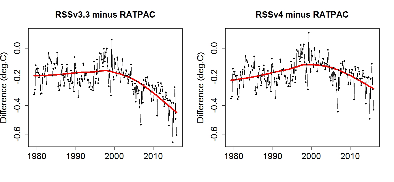
Please don’ t show those Christy graphs, falsely claiming to be “mid troposphere” (around 500 mbar?). It is not, it is the satellite TMT, a smeared out layer consisting of troposphere, tropopause and lower stratosphere. That’s a weakness of satellite data, it has poor vertical resolution, and the TMT has a fair share of stratospheric cooling contamination. Radiosonde and reanalysis data have vertical resolution, but Christy destroys it by smearing it out to emulated TMT.
Here is a comparison of Ratpac radiosonde data and CMIP5 data in three defined layers:
https://drive.google.com/open?id=0B_dL1shkWewaWnhjVzNyUDN5OWs
Conclusion: The warming in the free troposphere is similar to the models. The tropopause is warming slower than the models. The lower stratosphere is cooling faster than the models.
Also, the INM model is certainly not a good example. In the satellite era it’s global surface warming is only half of the observed temperature trend.
The INM model has a hefty energy imbalance at TOA. Since it doesn’t warm the surface and atmosphere, it probably disappears the heat into the deep ocean ( or melts the vast ice sheets).
I did a quick estimate, if the global imbalance followed the rcp4.5 scenario to 2100 and remained constant from there, the INM model would store heat enough to melt the entire ice sheets of Antarctica and Greenland by year 2250.
Olaf, not seeing that TOA energy imbalance in the published characteristics of either INMCM4 or INMCM5. And the hindcast of CM5 is not far off.
https://rclutz.wordpress.com/2018/10/22/2018-update-best-climate-model-inmcm5/
Ron, great post! Everyone, I recommend Ron’s update post on the Russian model (his second link) very worthwhile, I had not read it before now. Here is a good quote:
“One can conclude that anthropogenic forcing is unable to produce any significant impact on the AMO dynamics as its index averaged over 7 realization stays around zero within one sigma interval (0.08). Consequently, the AMO dynamics is controlled by internal variability of the climate system and cannot be predicted in historic experiments. On the other hand the model can correctly predict GMST changes in 1980-2014 having wrong phase of the AMO .”
Climate modeling is in its infancy and has a long way to go.
There ya go, colludin’ with them Russians again ! …. ok, I’ll just get my coat….
Ron,
Try KNMI climate explorer, thats where Christy gets his data from. They have INMCM4. The rcp4.5 trend 1979-2018 is 0.098 C/ decade for Global tas. If I remember right, the present TOA imbalance was 1.5 W/m2 and the final 2.3 W/m2 but the surface warming was very modest, only 1.0 C above present by 2100.
I’m quite convinced that have not published, discussed publicly, or thought of the TOA imbalance. If they knew, they would have scrapped the model and returned to the drawing board.
Olaf, your mean this:
“The precision achieved by the most advanced generation of radiation budget satellites is indicated by the planetary energy imbalance measured by the ongoing CERES (Clouds and the Earth’s Radiant Energy System) instrument (Loeb et al., 2009), which finds a measured 5-yr-mean imbalance of 6.5Wm−2 (Loeb et al., 2009). Because this result is implausible, instrumentation calibration factors were introduced to reduce the imbalance to the imbalance suggested by climate models, 0.85Wm−2” (Loeb et al., 2009).
This is circular reasoning. The CERES measurement is implausible, so a number is taken from climate models and claimed to be the standard. It looks like anything between 0.85 and 6.5 can be defended.
Ron,
You are citing an old paper. Nowadays CERES data are ground-truthed by Argo data (plus estimates of the other minor heat sinks) for the period 2005-2015, and thus totally independent of models.
The average imbalance for the most recent 10 years is 0.82 W/m2, and trending upward, suggesting values over 1.0 W/m2 right now.
Actually I have a graph with Ceres data, plus an own verification based on NOAA OHC:
https://drive.google.com/open?id=1FGyxbFhRcL5TQmoPO09I9HnsqVO4SW5N
Thanks for that graph Olaf. Yes there is a newer paper: Clouds and the Earth’s Radiant Energy System (CERES) Energy Balanced and Filled (EBAF) Top-of-Atmosphere (TOA) Edition-4.0 Data Product Norman G. Loeb and David R. Doelling January 2018
From Abstract:
“The Clouds and the Earth’s Radiant Energy System (CERES) Energy Balanced and Filled (EBAF) top-of-atmosphere (TOA), Edition 4.0 (Ed4.0), data product is described. EBAF Ed4.0 is an update to EBAF Ed2.8, incorporating all of the Ed4.0 suite of CERES data product algorithm improvements and consistent input datasets throughout the record. A one-time adjustment to shortwave (SW) and longwave (LW) TOA fluxes is made to ensure that global mean net TOA flux for July 2005–June 2015 is consistent with the in situ value of 0.71 W m−2. ”
From Uncertainty section:
“For CERES, calibration uncertainty is 1% (1σ), which for a typical global mean clear-sky SW flux corresponds to approximately 0.5 W m−2. The narrowband-to-broadband regional RMS error is 0.9 W m−2, determined by applying the narrowband-to-broadband regressions to cloud-free CERES footprints and comparing with CERES radiances. For clear-sky SW TOA flux, the radiance-to-flux conversion error contributes 1 W m−2 to regional RMS error (Loeb et al. 2007), and time–space averaging adds 2 W m−2 uncertainty. The latter is based upon an estimate of the error from TRMM-derived diurnal albedo models that provide albedo dependence upon scene type (Loeb et al. 2003).”
Olof, Which surface temperature estimate? They keep changing and with every change they go up. TMT estimates from satellite and radiosondes match fairly well, why don’t the models match at that elevation?
My point is, surface temperatures are modeled, and apparently not very well, since they are always changing. They have no special place, TMT is at least as good.
Finally, we do not have good data, for long enough, to validate any climate model, we need good data for at least 30 more years to see if any of the models are worth anything.
I do not believe it is physically possible to melt all of the ice on Antarctica in 200 years, I think you made an error. That said, if you were simply talking about storage of joules in the ocean, sure that is possible. But that much thermal energy is a drop in the bucket. The oceans have a huge heat storage capacity and an average temperature of 4C, which is the major difference in INM-CM4. I think the all the other models vastly over-simplify the oceans. Further, there is no particular reason why energy has to balance, in the short term, at the TOA. It has to balance over some length of time, but what length is that? We don’t know.
The models are so over-simplified as to be useless.
“TMT estimates from satellite and radiosondes match fairly well … ”
Thing is Andy – that is not so.
RATPAC A is trending at 0.218C/decade
UAH V6.0 is 0.035C/decade
(UAH TLT)
That is 1/6th of the warming trend revealed by the RATPAC A radiosonde series.
(and the little different TMT version will be no different)…..
http://www.drroyspencer.com/wp-content/uploads/MSU2-vs-LT23-vs-LT.gif
Even RSS V4 is 0.112C/decade (TTT)
Anthony, I find your plots unconvincing, when compared to John Christy’s plot which I know is an apples to apples comparison. Any global average can be manipulated via cherry picking, you need to present more than graphs to convince me the comparison is valid.
Particularly since there is almost no difference in the time series…
The spread is only about 0.2 C, about 1/5 of the annual variability.
The R2 for these trend lines would be minuscule.
“Particularly since there is almost no difference in the time series…”
Now I may be wrong, but what would you say if the trends were reversed?
If not you, then most on here would ‘cry wolf’ I strongly suspect.
So, what about the disparity between the previous MSU onboard NOAA14 and the present AMSU on NOAA15, since the change over in ’98?
That RSS has partially corrected for, but which UAH has not.
The RSS approach is pragmatic (since we do NOT know which sensor is wrong).
And UAH put all their faith in the present sat (because “Cadillac quality”).
Time will tell … but only when replaced again I suspect.
In short the tropospheric sat temp data is unreliable … from whatever source.
The problem with computing (yes not ‘measuring’) by multiple sources the same data from a single sensor.
There are thousands of sensors for the surface record …. where we live, and where greatest warming is taking place nocturnally over land – that tropospheric sensing does not see.
PS: Andy – what’s the secret of posting up an image here now, since that functionality disappeared to the rest of us a few months back?
Anthony, no secret, it’s just that I can edit the comment and insert an image. However, since the big change in software users without editing privileges cannot do this. The new system is very primitive, I’m sorry. I’ve had a lot of trouble with it also, hopefully WordPress is working on a solution.
There are differences between the satellite and radiosonde data, but they are much, much smaller than the differences between the models and the observations. And since the radiosondes and satellites are independent of one another we would expect there to be differences, right? Are you saying we should ignore observations and use the model results? Are the differences so large they cause a problem?
That troposphere chart is mine, but I have not updated it for a while.
However, I just looked at the topnotch, state of the art, king of reanalysis, ERA5, which now has data beginning in y 2000, and compared it with UAH TLT apples-to-apples:
https://drive.google.com/open?id=15gUj5AcD-gAqJ4HVYXu_3xYvUtwBvtOO
UAH TLT v6 loses about 0.14 C /decade vs ERA5.
RSS TLT v4 loses about 0.07 C/decade on ERA5, so it’s more right than UAH, but still trending to cool..
Its nothing special with ERA5, it just confirms all other radiosonde and reanalysis datasets, and demonstrates that UAH is a too cool “odd man out” in the AMSU-era
“That troposphere chart is mine, but I have not updated it for a while.”
Yes, thanks Olof – I thought it was.
“…. and demonstrates that UAH is a too cool “odd man out” in the AMSU-era”
Yes, it certainly does Olof!
The trend is estentially half of ERA5.
“you need to present more than graphs to convince me the comparison is valid”
Again, maybe not you Andy, however the same standard is usually followd by most denizens.
Correction
Not usually followed
Anthony, I see two trends slightly up and one trend slightly down. None of the slopes appear to be beyond the expected error in the measurements. Since majority doesn’t rule in science and you only have data for 20 years, what am I to make of this?
The difference between all these datasets and the model output (excluding INMCM4) is much, much larger, correct?
How can you verify that any of these datasets is significantly better than the others? Or more importantly, how can you verify these datasets are wrong and the models are correct?
“How can you verify that any of these datasets is significantly better than the others? ”
Because one is from radiosonde data – which is taken from thousands of individual balloon ascents and the other from one sensor aboard an orbiting satellite …. well 2 sensors which we know do not agree (both UAH and RSS say so).
Additionally 2 centres come out with a different answer from the exact same data!
Are we to go down the route of it’s the radiosondes that are wrong?
I suspect you are.
That makes no sense.
I do not talk of models.
The observational data is being “chosen” here to meet an ideological bias.
Pragmatism and common sense is massively weighted to the conclusion that …
UAH is a large cold outlier.
UAH does not agree with sonde data (which is where I came in to duspute your assertion).
RSS realise there is a distinct oroblem with the AMSU data relative to pre ’98 and we cannot be sure which data is wrong.
UAH deny the problem lies with the current sat.
Tropospheric temp data is badly fawed.
Troposperic temp data does not ‘see’ greatest warming taking place nocturnally over land (and over the Arctic).
Your posted graph does not convey reality of actual mid troposheric temp trend.
And in addition uses a misleading start and has no error bars.
Just the errors that would be loudly and rightly decried on here if published by the consensus side.
There is a word beginning with ‘h’ that describes that.
Anthony, You may be right regarding UAH versus radiosonde data and maybe RSS is better than UAH. I’m not speaking to that, just as you are not speaking to the models. In my case the differences between the radiosonde and the satellite datasets appear small and to you they appear large, it seems to be a matter of perspective.
I certainly agree that radiosonde data is better where we have it, but the coverage, especially in the Southern Hemisphere, is much less than the satellite datasets. There are problems with every estimate of global average temperature.
Temperature/Climate modelling is a bit like using leftovers from thanksgiving diner; let it cool down, warm it up when required and serve it to the unsuspected customers
http://www.vukcevic.co.uk/NH-Temp-Adj.htm
no hiding decline, is there?
Erm, in that 1975 -2015 graph of models versus observation do I notice 0.3 degs C rise in forty years? But wasn’t there 30 years cooling to 1970? So how does 1940 compare to today? Just asking.
CAGW Alarmism is a religious, political and financial movement not a scientific endeavour based on fact or observation. CAGW is based on faith and fervour and is immune to facts.
AMERICANS ARE WORRIED ABOUT CLIMATE CHANGE – this is not CAGW alarmism but a fact. Whatever the US sceptic community says, more Americans are becoming convinced that climate change is being caused by man’s activities: https://mankindsdegradationofplanetearth.com/2018/11/29/americans-are-worried-about-climate-change/
Some people are concerned about climate change and some think it is caused by humans. But, they do not think it is a priority:
A greater percentage of people believe in supernatural mumbo-jumbo than fear Gorebal Warming…
What’s really funny about this? 53% of those surveyed say they fear Gorebal Warming… But the highest ranking weather-related fear is ranked #34, “devastating drought” at 37.7%.
.. + 97% likes !
.. The climate has been “changing” for 4.6 Billion years ! Let me know when it STOPS changing, then I’ll be worried !
Pure surmise here; but it looks to me from figure 1 that circa 1993/4 there was a generalised shift in the algorithms/methodology in the computer models. (apart from the INM-CM4 model). This probably due to the dropping temperature found in the immediate preceding years. Not acceptable for the agenda?
I would love to know what that shift was and who initiated it.
Seems that these models are all micturating in the same container.
Alasdair,
The large Mt. Pinatubo (Philippines) volcanic eruption was in June of 1991. The eruption was large enough to affect the weather around the world for a few years, but it could be that the models over-estimate a impact a bit. Estimates of the impact vary, but the USGS claims it caused a 1 degree drop in global temperatures from 1991 through 1993.
https://pubs.usgs.gov/fs/1997/fs113-97/
Andy,
You say that the CO2 concentration in the atmosphere has increased by 27% since 1959 as measured at Muana Loa and, without being explicit, seem to imply that this increase is attributable to human activity.
How can anyone have a view on the extent to which the atmospheric CO2 increase is attributable to humans when:
1 The total anthropogenic emissions form a very small portion of global emissions on an annual basis
2 The uncertainty surrounding a number of non anthropogenic CO2 emissions, particularly from the oceans, is much greater the the absolute amount of human emissions, and
3 there is evidence to suggest that there has been a net warming of oceans over this time, given the size of the oceanic CO2 reservoir and the decreasing solubility of CO2 in water as temperature rises, how much of this atmospheric CO2 volume increase is attributable to increased ocean outgassing of CO2
4 for a considerable period since 1959 the world has been in a post Little Ice Age warming mode; there is evidence to suggest that atmospheric CO2 levels increase as a result of global temperature rise, how much of the post 1959 rise should be attributable to this
5 why is the CO2 level measured at Muana Loa a reasonable estimate of global CO2 concentrations
6 have you read “180 Years accurate CO2 – Gasanalysis of Air by Chemical Methods” by Beck? If so, any views
Best wishes
George
@ur momisugly George,
I agree with you.
Without anthropogenic co2 there is a strong possibility that the total atmospheric co2 would be dropping. I am surprised that they let such a large drop in co2 be in the record from last year May to September. ( 7 ppm/v) AGW can’t take credit if the yearly co2 anomaly drops to zero and coal plants are still running. The temperature doesn’t have to drop far for that to happen.
That 7 ppm/v drop was a net of atmospheric co2, it did not included all of the co2 that was released from May to Sept 2017 world wide. In other words, if we hadn’t produced any co2 (zero) during that time, co2 levels would have dropped 7 ppm/v. That’s a lot of co2… that’s 6 Billion Metric Tons more than we produce in a year. Where did it go? And why did it come back?
The simplistic answer from AGW is, “it’s summer in the NH”. It never becomes summer in the SH or it doesn’t count?
George, I don’t think anyone can say for sure how much of the additional CO2 today is due to human emissions, but some of it is. We know fairly precisely how much we put in the air, since we have records of coal, oil and natural gas sold. We also know the 13C/12C ratio has changed, suggesting some of the added CO2 is due to fossil fuel burning. Uptake of the added CO2 in the biosphere, which is growing larger, and in the oceans, reduces the additional CO2, but some remains in the atmosphere.
https://myweb.rollins.edu/jsiry/isotopes.html
Andy
The increase in atmospheric Co2 is about 4% anthropogenic. See Harde 2017. you will have to go to( https://hhgpc0.wixsite.com/harde-2017-censored) to see Harde’s response to Kohler’s attempted rebuttal because the journal wouldn’t publish it. Another clear explanation of this as well as a clear rebutal of the IPCC position on anthropogenic contributions to atmospheric content is
https://edberry.com/blog/climate-physics/agw-hypothesis/contradictions-to-ipccs-climate-change-theory/
I think even the second box of your growing uncertainty diagram should be starting to gray out as there is reason to believe that the atmospheric content is naturally controlled and the anthropogenic part is just like any other small source. If it cools off the amount of human CO2 will not change the reduction in the atmosphere.
George,
It’s possible that up to half of the CO2 rise was natural. However, some of it, probably 50-75% is anthropogenic.
Regarding your specific points:
1. Humans only account for about 3% of the annual CO2 sources. However, we are moving carbon from geologic sequestration (fossil fuels) into the active carbon cycle primarily in the form of CO2. It probably takes decades to hundreds of years for that CO2 to become re-sequestered.
2. Correct. Our contribution is smaller than the uncertainty.
3. There’s clear evidence of this in the Law Dome Antarctic ice core (MacFarling-Meure, et al., 2006). Despite rising emissions, atmospheric CO2 stopped rising and possibly declined from 1945-1955.
4. I think about 40% of the rise could reasonably be attributed to post-LIA warming. But this is almost impossible to prove.
5. Mauna Loa measurements have been confirmed from other sites.
6. Very interesting paper. There are some problems with it, but it shouldn’t be ignored.
One of the problems is that every pre-industrial CO2 estimate, not derived from Antarctic ice cores is largely ignored. Direct atmospheric measurements (like Beck), plant stomata and Greenland ice cores all indicate higher and more variable pre-industrial CO2 levels. Multiple plant stomata chronologies indicate that 300-350 ppm CO2 was common throughout the Holocene.
Of course the best thing about models is that using them can get you the results you ‘need’ without any of the problems of dealing with reality that often fails to do so.
The next best thing is they make it so easy to play ‘find the lady ‘ without any of the hardwork involved in field work or actaul experiments .
So you can see why the intellectually light weights who so often have found comfortable home in climate ‘science ‘ like them.
So, if you think you are better than the ‘lazy’ climate scientists, then what methodology are you suggesting that is superior to the current modelling for predicting the future impact of global planetary temperature rises?
Please list 10 concrete suggestions here.
Ivan, no one has come up with any methodology for predicting the future impact of global warming with sufficient accuracy to know if it will benefit or harm mankind. Right now the best prediction is it will not matter at all, that should be the null hypothesis.
Perhaps with 30-50 years more data we will be able to come up with a model that can be validated and produce a tight set of predictions that are believable. But, the honest answer today is that we don’t know.
From what I have learned, primates (including homo sapiens) have survived cold periods and thrived during warm periods. These primitive and unsophisticated animals have thrived during periods warmer than that being forecast.
Is it wrong to think that modern homo sapiens with their increasing technological sophistication can not also manage to survive and thrive during another warm period? Sure there will be some dislocation and other changes. As related to a species, change can be good, it can speed up evolution.
Why do all the “studies” assume Armageddon or that the Four Horsemen of the Apocalypse will be riding the land? They are all doom and gloom. What ever happened to the quote “Necessity is the mother of invention”? Do all the current climate scientists and politicians really believe that we already know everything we can ever know? That there will never be any further technological or societal advances that will help ameliorate climate change problems?
A question about economics. If people along the coasts must relocate due to sea level rise will this grow the economy or cause it to decrease? We currently rebuild after fires, why not after sea level rises? To spread this out, why don’t politicians just up and ban any further development on the coasts as of tomorrow? No new building within 20 miles of a coast line! If they truly believe this is going to happen they are being fools to not start reckoning with the consequences they are forecasting. Voters should be demanding action now not after a problem arises. A case in point, should they not be planning to move Washington, D. C., maybe to the center of the U.S.? Better yet, why don’t we start planning for the next ice age and start moving people away from those areas that may be covered in ice? The precautionary principle should apply to this scenario too.
I am old enough to remember when the Boeing 707 was latest and absolutely greatest way to fly. I remember looking up and seeing Sputnik in the sky and wondering where we might be heading. I remember telling my boss that historians will treat the Internet Revolution as they do the Industrial Revolution and I still believe that. I still believe that nuclear, both fusion and fission, will be way of the future.
In other words, all these doom and gloom studies assume that human kind will remain stagnant with no further innovations. Done by Luddites all. I don’t believe any of them.
Ivan Kinsman:
With respect to future global planetary temperature rises, there are two components:
1. Earth’s natural recovery from the Little Ice Age cooling: ~.05 deg. C. per decade
2. The amount of Sulfur Dioxide aerosols in the atmosphere, of both volcanic and anthropogenic origin: ~.02 deg. C. of temp. change for each net Megaton of change in global SO2 aerosol emissions.
Future temperature changes CANNOT be accurately modeled (predicted) because of the random nature of volcanic eruptions.
However, the continued reduction in anthropogenic SO2 aerosol emissions will cause temperature to rise, at the rate noted above (an unfortunate side effect of Clean Air efforts).
On the other hand, a simple way of reversing much of the anomalous warming to date would be to increase SO2 aerosol emissions via the increased burning of fossil fuels.
None of the above comments can be refuted, and all can be proven, but I would predict that they will simply be ignored, as long as possible.
I wonder if there is a way to transfer both U.S. Fourth National Climate Assessment (NCA4) Volume I and U.S. Fourth National Climate Assessment (NCA4) Volume II to toilet paper? Perhaps donate the proceeds to those that are forced to choose between eating or heating during the winter.
Ivan Kinsman, try an Ouija Board, it will out perform all other methodologies for predicting the future.
This is a huge step for mankind to get real professionals here. So it is possible that the obsessed skeptics will lose their total leadership in this forum.
I was around some researchers in graduate school that worked on gas exchange because it was a good symptom (measure) of energy flow (productivity). This was well before the hysteria.
https://nca2018.globalchange.gov/chapter/9/ (KM 1 Ocean Ecosystems)
“Second, it increases the concentration of hydrogen ions, acidifying the water. Acidity is measured with the pH scale, with lower values indicating more acidic conditions……For simplicity, the terms ocean acidification and acidifying will refer to the suite of chemical changes discussed above……. Furthermore, ocean ecosystems are becoming increasingly NOVEL (CAPS MINE), meaning that knowledge of current ecosystems will be a less reliable guide for future decision-making (Ch. 28: Adaptation, KM 2)…..The implications of the projected changes in fisheries dynamics on revenue 94 ,96 and small-scale Indigenous fisheries remain uncertain.97”
Go back to the chapter’s executive summary–“Even without directly accounting for climate effects, precautionary fishery management and better incentives can increase economic benefits and improve resilience.”
In their citations for “dead zones”
https://onlinelibrary.wiley.com/doi/abs/10.1111/gcb.12754
Authority for effect on “dead zones” Paywalled.
Abstract boilerplate, no data or analysis
https://www.nature.com/articles/ngeo1297
“ Model simulations, using data collected from the northern Gulf of Mexico, however, suggest that the drop in pH since pre-industrial times is greater than that expected from eutrophication and ocean acidification alone.” Based on 0.05 change in pH units, modeled. I am looking at 24 hour graphs of pH for inshore Texas waters. Extremes– 8.22-8.90, 8.39-8.42 (dinoflagellate bloom). These are inshore, less fluctuation over the open ocean because it is on average not very productive.
Increased “dead” actually not so dead zones might benefit some like which I saw once—-.
Craig, J. K., et al. 2010. Habitat use of cownose rays (Rhinoptera bonasus) in a highly productive, hypoxic continental shelf ecosystem. Fisheries Oceanography. 19(4):301-317.
First, they don’t do their homework and second they write and logic at a subcollege level, no offense to subcollege, must be better comparison. NOVEL means they don’t know what is going on which they seem to admit. Louisiana could feed a good bit of the nation with their erroneously called “dead zones.” Correct terms are azoic, hypoxic, sometimes anoxic. Of course old out of date terminology, some rediscovery.