Guest essay by Antero Ollila
I have written blogs here in WUWT and represented some models of mine, which describe certain physical relationships of climate change. Every time I have received comments that if there is more than one parameter in my model, it has about no value, because using more than four parameters, any model can be adjusted to give wanted results. I think that this opinion originates from the quote of a famous Hungarian-American mathematician, physicist, and computer scientist John von Neumann (1903-1957). I found his statement in the Wikiquote:
“With four parameters I can fit an elephant, and with five I can make him wiggle his trunk”.
I do not know what von Neumann meant with his statement, but I think that this statement can be understood easily in the wrong way. I show an example in which this statement cannot be applied. It is a case of curve fitting. My example is about creating a mathematical relationship between the CO2 concentration and the radiative forcing change (RF). Myhre et al. have published equation (1) in 1988
RF = 5.35 * ln(C/280) (1)
where C is the CO2 concentration in ppm. Somebody might think that clever scientists have proved that this simple equation can be deduced by a pen and paper, but it is impossible. The data points RF versus CO2 concentrations have been calculated using the BBM (Broad Band Model) climate model and thereafter Eq. (1) has been calculated using a curve fitting procedure. There are no data points in the referred paper but only this equation and a graphical presentation. The BBM analysis method is the most inaccurate method of the radiative transfer schemes. The most accurate is the LBL method (Line-B-Line), which I have used in my calculations. Anyway Myhre et al. have shown in their paper that BBM and LBL methods give very closely same results.
I have shown in my paper that I could not reproduce Eq. (1) is my research study: https://wattsupwiththat.com/2017/03/17/on-the-reproducibility-of-the-ipccs-climate-sensitivity/
I carried out my calculations using the temperature, pressure, humidity, and GH gas concentration profiles of the average global atmosphere and the surface temperature of 15 ⁰C utilizing the LBL method. The first step is to calculate the outgoing longwave radiation (OLR) at the top of the atmosphere (TOA) using the CO2 concentration of 280 ppm. Then I increased the CO2 concentration to 393 ppm and calculated the outgoing LW radiation value. It happens in two steps: 1) transmittance or a radiation emitted by the surface and transferred directly to space, and 2) radiation absorbed by the atmosphere and then reradiated to space. The sum of these components shows that the OLR has decreased 1.03 W/m2 due to the increased absorption of the higher CO2 concentration. The other points have been calculated in the same way.
The values of the four data pairs of CO2 (ppm) and RF (W/m2) are: 280/0; 393/1.03; 560/2.165; 1370/5.04. Using a simple curve fitting procedure between the CO2 and the term ln(C/280), I got Eq. (2):
(2) RF = 3.12 * ln(C/280)
The form of equation is the same as in Eq. (1) but the coefficient is different. For this blog I carried out another fitting procedure using the polynomial of the third degree. The result is Eq. (3)
(3) RF = -3.743699 + 0.01690259*C – 1.38886*10-5*C2 + 4.548057*10-9*C3
The results of these fittings are plotted in Fig. 1.

As one can see, there is practically no difference between these fittings. The polynomial fitting is perfect, and the logarithmic fitting gives the coefficient of correlation 0.999888, which means that also mathematically the difference is insignificant. What we learned about this? The number of parameters has no role in the curve fitting, if the fitting is mathematically accurate enough. The logarithmic curve is simple, and it shows the nature of the RF dependency on the CO2 concentration very well. The actual question is this: Are the data points pairs calculated scientifically in the right way. The fitting procedure does not make a physical relationship susceptible and the number of parameters has no role.
So, I challenge those who think that an elephant can be described by a model with four parameters. I think that it is impossible even in two-dimensional world.
I don’t think the issue is necessarily that models with more parameters are wrong, just that the more parameters a model has, the more places it can be wrong.
A classic example is RADIATION.F in the GISS GCM called ModelE. This one piece of spaghetti Fortran code has thousands of baked in floating point constants, many of which have absolutely no documentation, most notably, those related to atmospheric absorption coefficients.
On the other hand there’s the SB equation for a gray body, which has only one parameter called the emissivity. For calculating the yearly average relationship between the surface temperature of a region of the surface and the emissions into space above that region, it fits almost perfectly using an effective emissivity of about 0.62 +/- 5% across all regions of the planet from pole to pole.
co@isnotevil
Is that emissivity for a particular CO2 concentration?
I agree with taking a grey body approach, mainly because the atmosphere is not a black body in the relevant wavelengths.
How then does ‘darkening’ the atmosphere by adding CO2 affect the emissivity?
Next point: There are two contributors to the atmospheric temperature just above the ground: convective heat (Hc) transfer from the hot surface and radiated or re-radiated infra-red energy.
Regular CO2
Hc + ir => Air temperature
It is claimed that as the CO2 concentration increases, the temperature of the surface air will increase as the emissivity of the atmosphere increases in both directions: up and down.
Hc + CO2 => HC
High CO2
HC + ir => Higher air temperature
What is strange is that if we take the opposite tack, that of reducing the CO2 concentration and reducing the emissivity of the atmosphere to a low value, the equation for air temperature still has two components:
Low CO2
Hc + ir => Air temperature
but the atmosphere will have lost its ability to cool radiatively (low emissivity).
The reason ir thermometers have a scalable emissivity function is to be able to get the correct temperature from the IR being radiated. When the surface is like polished silver, it emits nearly no IR at all and the IR device reads Low. A correction is made to report a higher temperature (the real temp) by adjusting the emissivity button.
Polishing metal to a mirror is not different from an atmosphere that loses its ability to cool by radiation. The Hc or HC contribution will continue to be made, of course, and the atmosphere will have lost the ability to radiate that energy. The air temperature will then rise inexorably until some gas starts to radiate or the air heats the surface sufficiently at night.
If you do your calculations using an emissivity of 0.10 instead of 0.62, what air temperature must be reached in order to dispose of the same amount of energy as currently reaches the surface? It will be a heck of a lot more than 15 C at the surface.
It is generally true that in order to cool a hot body more effectively, the radiating function – the emissivity – has to increase. Adding CO2 to the atmosphere increases the emissivity and is therefore bound to lower the temperature until it is again in net radiative equilibrium. It is very difficult to find CAGW in the physics of a radiating atmosphere (even without the clouds). Check Trenberth’s diagramme. The effect of Hc is missing and hidden among the radiative weeds.
Crispin,
The emissivity changes slightly with increasing CO2 concentrations and it’s this slight change in emissivity that’s equivalent to the 3.7 W/m^2 of post reflection solar forcing said to arise from doubling CO2. Technically, only solar energy forces the system. Changing CO2 concentrations is a change to the system itself and not a change to the forcing, although any change to the system can be said to be EQUIVALENT to a specific change in the forcing keeping the system constant.
Quantitatively, the effective emissivity can be calculated as 1 – A/2, where A is the fraction of NET surface emissions that are absorbed by atmospheric GHG’s and clouds, considering that half of this must eventually be emitted into space and the remaining half re-emitted back to the surface. The absorption coefficient A, can be calculated as the cloud fraction weighted absorption, where with no clouds, all absorption is by GHG’s and with clouds, absorption is dominated by the liquid and solid water in clouds, which like GHG’s eventually re-radiate that energy up and down in roughly equal parts.
We should only be concerned with the AVERAGE temperature of the radiating surface, which is nearly coincident with what we consider the ‘surface’ to be. The temperature of the atmosphere doesn’t drive the surface temperature, but is a consequence of the surface temperature which is determined by its own specific radiative balance. Convection affecting air molecules in motion (i.e. their kinetic temperature) is irrelevant to the radiative balance as the translational motion of air molecules doesn’t participate in the RADIATIVE balance, but is the source of the energy required to obey the kinetic temperature lapse rate dictated by gravity. Note that whatever effects non radiative transports like latent heat and convection have on the surface temperature is already accounted for by that temperature and its corresponding BB emissions, thus has a zero sum contribution to the NET radiation of the surface whose temperature we care about. This is something else that Trenberth’s energy balance diagram is misleading about, especially since he refers to the return of non radiative energy as ‘back radiation’.
Crispin,
One other point is that it’s not the emissivity of the atmosphere that’s being modelled, but the emissivity of a gray body model of a system whose temperature is that of the surface and whose modelled emissions are the fraction of emitted surface energy that’s eventually radiated into space. Any energy emitted by the atmosphere was emitted by the surface some time in the past and any energy emitted by the surface and absorbed by the atmosphere can be re-emitted into space or back the surface only once. The ultimate time or place where energy emitted by the surface ultimately leaves the planet or returns to the surface is irrelevant.
Increasing CO2 concentrations decreases the effective emissivity and the energy that was not otherwise emitted must be returned to the surface, contributing to making it warmer than it would be otherwise.
Co2isnotevil said
“Increasing CO2 concentrations decreases the effective emissivity and the energy that was not otherwise emitted must be returned to the surface, contributing to making it warmer than it would be otherwise.”
Battisti and Donohoe say the exact opposite happens in the long run in their 2014 study that says after a period of time (decades)……”and the negative LW feedbacks that strongly increase OLR with warming” The name of the study is
“SHORTWAVE AND LONGWAVE RADIATIVE CONTRIBUTIONS TO GLOBAL WARMING UNDER INCREASING CO2” They say it takes decades for the feedbacks to kick in but that eventually it is the SW radiation which causes global warming not the LWIR. The authors go on to say “Only if the SW cloud feedback is large and negative could the SW coefficient become small and the resulting energy accumulation be dominated by reduced OLR. That is all they say about clouds in the report but Battisti admits that he doesnt have a good handle on clouds.because the media summary copy which I assume was approved by the authors including Battisti before being released to the media said “clouds remain one of the big unknowns under climate change”. So if that is true and everybody seems to agree because noone can model clouds properly and no one has any equations for the clouds(in other words there is no theory that explains the clouds relationship to IR forcing then why in the hell havent all the climate scientists told the politicians that because clouds are too much of an unknown we should do nothing until we can figure it out.
THEY HAVENT DONE THAT. INSTEAD THEY TOLD THE POLITICIANS THAT OUR MODELS PREDICT LARGE INCREASES IN GLOBAL WARMING THEREFORE YOU SHOULD ACT and we are all suffering financially because of it.
I believe THAT ALL OF YOU ARE WRONG and that Willis is right about his convection with clouds theory having everything to do with it , assuming that changes in the sun cause only minor climatic changes (which noone has been able to prove or disprove). WHAT A MESS
Changing CO2 concentrations is a change to the system itself and not a change to the forcing, although any change to the system can be said to be EQUIVALENT to a specific change in the forcing keeping the system constant.
How refreshing to see that stated.
We have a GH effect in our atmosphere and CO2 has a contribution of about 13 %. By increasing the CO2 concentration, the magnitude of the GH effect will increase, because the present absorption in the atmosphere is at the level of 90 %. The only way that CO2 concentration increase would have no effect, is the negative water feedback effect. According to the measurements, the amount of water vapor in the atmosphere is practically constant. Certainly it is not positive as calculated in computer models.
aveollila,
The 90% absorption of surface emissions is incorrect. This comes from Trenberth’s balance and if you ask him where this came from, he has no good answer, My HITRAN based analysis tells me that the clear sky absorbs between 60% and 70% (avg 65%), is all by GHG’s and dependent on water vapor content. Nominally, water counts for more than 1/2 of this, CO2 is a bit more than 1/3, Ozone is most of the rest and a few percent arises from CH4 and other trace gases. Cloudy skies absorb on average about 80%, much of which is by liquid and solid water in clouds and would be absorbed independent of GHG concentrations between clouds and the surface. The planet is nominally 2/3 covered by clouds, so the total absorption fraction of surface emissions is 0.33*0.65 + 0.66*0.80 = 0.74, or about 74%.
If 90% was correct, then 350 W/m^2 of the 390 W/m^2 of surface emissions is absorbed, leaving 40 W/m^2 passing through the transparent window. This requires 200 W/m^2 more emissions into space to be in balance, which can ONLY come from the 350 W/m^2 of absorption, leaving 150 W/m^2 to be returned to the surface, which added to the 240 W/m^2 of solar input adds up to the 390 W/m^2 of emissions. What this would mean is that only 43% of the energy absorbed by the atmosphere is returned to the surface while 57% of atmospheric absorption escapes out into space, even as the IPCC ambiguous definition of forcing requires 100% of what’s absorbed to be returned to the surface. Both violate the geometric constraint where half must be returned to the surface and the remaining half is emitted out into space.
If 74% is absorbed, the total is about 290 W/m^2, leaving 100 W/m^2 passing through which requires additional emissions of 140 W/m^2 of the 290 W/m^2 absorbed to be in balance, leaving 150 W/m^2 returned to the surface which added to 240 W/m^2 offsets the 390 W/m^2 of emissions and is much closer to the required 50/50 split. A more precise analysis based on weather satellite imagery converges even closer to the 50/50 split dictated by geometric factors.
Many are confused by Trenberth’s latent heat and thermals whose effect is already accounted for by the average temperature and its average emissions and offset by the return of latent heat and thermals back to the surface which Trenberth incorrectly lumps into his bogus ‘back radiation’ term. It’s crucially important to distinguish between energy transported by matter which is not part of the RADIATIVE balance and can not leave the planet (man made rockets not withstanding) and the energy transported by photons which exclusively comprises the RADIATIVE balance,
co2isnotevil,
Two quick questions for you that have been vexing me.
First, why 50/50 between surface and space for atmospheric radiation? The only place where the surface would equal 50% is right at the surface. That is, if we consider that any individual molecule can radiate spherically in any direction, the cross section of this sphere occluded by the earth’s surface diminishes from 50% as you ascend in altitude. Or, is this reduction so insignificant that it’s not worth refining? Just curious.
Secondly, going back to a previous discussion in which, if I remember correctly, you argued that IR couldn’t thermalize through collisions since it was internal molecular energy …energy like stretching, or bending or whatever rather than kinetic (sorry, can’t remember the correct terms off the top of my head). I’m not sure I’ve understood your position correctly…but if I’m close, it leads me to ask why we accept that some types of EMR can thermalize, but not LWIR? Microwaves immediately come to mind. (Note, if I’m so far out in left field with my misunderstandings, then just tell me. I haven’t really had a lot time to dig into this in my thoughts to make sure I’m asking a sensible question, so I’m “emotionally prepared” for you to tell me to go pound sand.) 🙂
rip
Rip,
The 50/50 split is a consequence of geometry. The area of the top boundary with space is about the same as the area of the boundary with the surface where energy enters only from the surface boundary, but leaves through both boundaries comprising twice the total area upon which energy arrives. To be clear, the running global average is not exactly 50/50 and varies a couple percent on either side and locally, clouds can modulate the ratio over a wider range. It makes sense that with sufficient degrees of freedom, a system like this will self organize to be as close to ideal as possible, as this minimizes changes in entropy as the state changes. This is a consequence of deviations from ideal increasing entropy and the 50/50 split, as well as conformance to the SB Law describing a gray body emitter are both ideal behaviors.
Regarding thermalization, the only possible way for CO2 to thermalize vibrational energy is to convert it to rotational energy that can be POTENTIALLY shared by a collision. These rotational bands are microwave energies and this energy represents the spacing of the fine structure on either side of the much higher energy vibrational modes. There’s no possible way to convert all of the energy of a vibrational mode into the energy of translational motion in one transaction since Quantum Mechanics requires this to be an all or nothing transfer, which can only happen by the collision with another GHG molecule of the same type where the energization state flips. Small amounts can be transferred back and forth in and out of rotational modes and is what spreads out the fine structure on either side of primary absorption lines. Rotational modes can theoretically be transferred to arbitrary molecules, but once more, this is an all or nothing conversion, although high N rotational modes are possible where less than N can be transferred. In general though, the transfer of state energy by collision is limited to collisions of like molecules where state is exchanged.
The only thermalization mode that makes sense is when an energized water vapor molecule condenses upon a water droplet, warming that droplet.
Another point is how well known are the values of the parameters.
If the values are well known and tightly constrained, there is not a problem.
If the value is so poorly known that the modeler is free to put in whatever value makes his model work, then we have problem.
…we have a winner
Agree. And the CMIP5 models have many more ‘parameters’ than 4.
And a great many of those parameters are poorly known at best. The classic example is aerosols,. As you go back into time, we have very little knowledge how much aerosols have released in any given year. What the compositions of those aerosols were, and from where they were released.
As a result you can plug a wide array of numbers into your model, with equal likelihood of entering the correct amount.
If the model isn’t given you the result you want, just tweak the amount of aerosols until it does.
CO2isnotevil, I posted this before.
In 1954, Hoyt C. Hottel conducted an experiment to determine the total emissivity/absorptivity of carbon dioxide and water vapor11. From his experiments, he found that the carbon dioxide has a total emissivity of almost zero below a temperature of 33 °C (306 K) in combination with a partial pressure of the carbon dioxide of 0.6096 atm cm. 17 year later, B. Leckner repeated Hottel’s experiment and corrected the graphs12 plotted by Hottel. However, the results of Hottel were verified and Leckner found the same extremely insignificant emissivity of the carbon dioxide below 33 °C (306 K) of temperature and 0.6096 atm cm of partial pressure. Hottel’s and Leckner’s graphs show a total emissivity of the carbon dioxide of zero under those conditions.
http://www.biocab.org/Overlapping_Absorption_Bands.pdf
mkelly,
Clouds are complicated because they affect both the input side by modulating the albedo and the output side by modulating the transparency of the atmosphere which also warms the surface as the transparency decreases.
Your hypothesis can’t explain why we only see about a 3 db (50%) attentuation in those absorption bands where the HITRAN line data tells us that the probability of absorbing a photon emitted by the surface is nearly 100%. If the emissivity of the GHG molecules is as low as you say, what’s the origin of all the energy we see at TOA in those absorption bands?
Also, the emissivity of the atmosphere is insignificant, relative to the emissivity of the surface itself, at least without accounting for energized GHG molecules and the water in clouds. GHG molecules act more like a mismatched spectrally specific transmission line between the surface and space.
I read that study there were significant questions with it. Until someone else does an actual experiment this is all conjecture the study author only did elementary calculations. and even those were confusing. . The study is a joke compared to a real scientific report. We need better than that to expose the hoax.
CO2, It is not my hypothesis but Hottel’s. He wrote books on radiative heat transfer and his charts are used in design calculations for combustion chambers.
If you don’t like Hottel, then please tell me what is the emissivity of CO2 in our atmosphere at present concentrations.?
I agree with the comments of CO2isnotevil and Alan Tomalty. The study referred by mkelly is not convincing and its theory is not generally accepted by other scientists as far as I know. I rely on the Spectral Calculator LBL-method and the HITRAN database. The overall results of the outgoing LW radiation as well as the downward overall radiation matches with observations. For me it is the best evidence about the calculation basis.
@ur momisugly mkelly
what’s this strange “atm cm of partial pressure” unit?
does this means you have to multiply by the actual thickness (kilometers for the atmosphere) relative to a cm standard (km/cm = 10^5)?
In which case, well, you could easily have both a “total emissivity of almost zero” in the standard case, and a significant emissivity in the real world.
Paqyfelyc here is a Hottel chart I found on line. I hope this answers your question.
mkelly,
“If you don’t like Hottel, then please tell me what is the emissivity of CO2 in our atmosphere at present concentrations.?”
Emissivity is a bulk property and isolating the emissivity of a trace gas in the atmosphere is a meaningless exercise. GHG’s essentially emit everything that they absorb, so in an absorption band, the effective emissivity is 1.0 and outside the absorption bands, the effective emissivity is 0. It’s also crucial to understand that when I talk about the emissivity, I’m talking about the bulk emissivity of a system comprised of a surface emitting energy corresponding to its temperature and an atmosphere between the emitting surface and space where the NET emitted energy is observed.
The idea that there is any NET thermalization of CO2 is absolutely wrong. While there’s conversion between the vibrational states and rotational states of CO2, this goes both ways. The fine structure of CO2 absorption lines is very clear about this having lines on both sides of the primary resonance. A line at a lower frequency means that energy was taken from a rotational state to make up the difference, while a line at a higher frequency means that the excess energy was put into a rotational state. The fine structure is relatively symmetric around the primary resonance which means that energy is added to and removed from rotational states in nearly equal and opposite amounts.
Note that there is some NET thermalization from water vapor, which happens when an energized water vapor molecule condenses upon a liquid water droplet and the state energy warms the resulting droplet.
@mkelly
the graph doesn’t say what this unit is. Just hint at being bar*cm, not bar/cm.
And you are not supposed to use bar nor cm, anyway, SI units are pascal (= newtons/m²) and meters. bar*cm would some sort of newton/meters, that’s the unit for a spring stiffness, which also apply to a air spring. Is that the context of Hottel work? I don’t know. Do you?
“If you don’t like Hottel”
There is nothing wrong with Hottel. The problem is Nasif Nahle’s elementary misreading of the graph which mkelly seems determine to blindly propagate. The units of bar cm aren’t intended to suggest work done. The emissivity of a gas basically depends on the mass (volume*density) per unit area. 1 bar cm on that graph means the emissivity of a layer 1 cm thick at 1 atm pressure. So the bottom curve, .06 bar cm, is the emissivity of a 0.6 mm thick layer of pure CO2 at 1 atm. Nasif Nahle has no idea how to read this plot, and neither, it seems, does mkelly. The relevant curve for the atmosphere would be right at the top of that plot.
@mkelly @Nick Stockes
never thought i would have to thanks Nick, but he fact is, I do.
400ppm of a few km atmosphere is in the meter range, so
“The relevant curve for the atmosphere would be right at the top of that plot”, indeed. That is, close to 0.2 at usual temperature ; and that’s NOT almost zero, for emissivity
wait till u find out that CO2 is a russian bot.
It is well known quote. Fermi asked Neumann to evaluate mathematical model. Neumann asked how many FUDGE parameters are there; when Fermi said “5”, Neumann tossed out model and said that. The key is the word “Fudge”, i.e. not determined by experiment.
A model with just a few parameters can be parameterized to fit historical observations without having predictive capabilities. Climate models got many parameters.
The models have trouble getting the historical observations correct.
It is interesting to see the enormous range in energy fluxes in the CMIP5 models (CMIP5 =Climate Model Incomparison Project) used by IPCC in their Assessment Report 5.
The energy balance over land and oceans: an assessment based on direct observations and CMIP5 climate models – Wild et al 2014
Here are some examples of the range of energy fluxes that is spanned out by the models (See Table 2: Simulated energy balance components averaged over land, oceans and the entire globe from 43 CMIP5/IPCC AR5 models at the TOA, atmosphere, and surface)
Surface (All units: W/m2): Solar down: 18.6
Solar up: 10.5
Solar net: 17.2
Thermal down: 18.5
Thermal up: 11.8
Thermal net: 15.7
Net radiation: 17.2
Latent heat: 13.9
Sensible heat: 13.1
(Averages are taken over the period 2000–2004)
Taking into account that the current energy accumulation on earth is estimated from observation of ocean warming to be approximately 0.6 W/m2 (Ref.: “considering a global heat storage of 0.6 W m–2» ref.: IPCC;AR5;WGI;page 181; 2.3.1 Global Mean Radiation Budget), I think it is fair to assume that the models would have been all over the place withou heavy parameterization.
The spread demonstratest that these models cannot all be be right. To the extent that some of these models may seem right, they may also seem right for wrong reasons – tuning and parametrization to get a desired result.
AGW specializes in Fudge. They (the climate scientists) are the biggest candy makers of all time. However we will eventually take their candy away from them.
That’s pretty much what “macro economy” has been doing…
That approach is too simple.
“I do not know what von Neumann meant with his statement”
It was just a metaphor, but to put in in tangible terms:
The 4 parameters are height, width, length and mass. The fifth is the wiggle rate of its trunk.
So would the LXWXH and mass of a mouse allow you to recreate an elephant?
“So would the LXWXH and mass of a mouse allow you to recreate an elephant?”
Yes, if you can set those four parameters as you wish rather than as determined by experiment.
If you replace the mouse model with an elephant model, the same 4 parameters can produce a really tiny elephant. Keep in mind that I’m talking about the model of an average elephant (or mouse), not the model of a specific instance of a real animal which would require far more parameters.
This illustrates the problems with GCM’s as they try to project the EXACT weather going forward in order to predict trends in the average climate. It’s much more accurate and far easier to use a simpler model that predicts the average based on macroscopic properties.
This would be a pointless exercise as there are so many elephants in the room already that there is little wiggle room remaining.
Since we’re talking about the elephant in the room:
CO2isnotevil. This explanation makes sense. By using so general terms it is possbile to describe the major features of an elephant.
Antero Ollila
It’s just metaphor with a dash of hyperbole to make it memorable and a bit snarky.
Regarding that 5.35 ln (CO2 final/CO2 original), Clive Best got a value of
6.6 , which was “.. approximately derived just from changes to the emission height with increasing CO2.”
http://clivebest.com/blog/
Adding parameters, or changing the function to fit is an exercise in what my advisor called bumpology. The key is without some physical reason why a curve is quadratic or logarithmic, it is all just a fitting exercise.
First comes the physical understanding, then the fitting.
The problem in complex systems like climate, we often don’t know the whole physics.
We know quite well that the dependency of RF on the CO2 concentration is not linear. By applying the method what I described we can calculate the RF value per a CO2 concentration. In order to utilize these results, we need to carry out a mathematical fitting. And right here these comments pop up that it is just a fitting exercise, because there is no physical reason or connection. That is not so. There is a physical connection between each RF per CO2 concentration values. The curve fitting procedure does not destroy this physical connection. Utilizing the curve fitting we can find out a simple equation between the CO2 concentration and RF value. And this equation is very useful and in this case it is perhaps the most important equation or formula in the climate change science.
Antero Ollila
It that case, the physical relationship is known, the curve fit is just a way of representing that relationship in a compact manner.
It is a completely different issue when climate models, with many parameters, are tuned to match historical data and claimed to have precision in prediction based largely on that explicit and implicit tuning.
Re aveollila
**Utilizing the curve fitting we can find out a simple equation between the CO2 concentration and RF value. And this equation is very useful and in this case it is perhaps the most important equation or formula in the climate change science.**
This curve relates CO2 levels to Radiative Forcing. Correct?
However, these are calculations? Correct?
Now I noticed that these “forcings” are used to calculate future additional warming by CO2 as the CO2 increases to the end of the century.
Are there any measurements of the warming by the changes in CO2?
Or are we assuming that the warming increases as the “calculated” forcing increases?
Can you describe an in-situ experiment whose data matches the model curve? Are there published papers with results?
This may work, but physically if we don’t have the mechanism we can not eliminate the possibility that the CO2 and T aren’t both the effect of an unknown and unmeasured separate cause.
Antero,
One thing that neither the LBL or BBM calculation of RF handles is clouds. The influence of clouds reduces the incremental effect of increasing GHG concentrations since the clouds would be absorbing that energy anyway and the net effect from a cloud or GHG absorbing energy is roughly the same relative to the NET energy balance. This reduces the global RF as a function of CO2 concentrations by as much as a factor of 2.
J said “we often don’t know the whole physics”.
i would conjecture that we know very LITTLE of the physics.
To Jeanparisot.
I have not seen any simple study showing the experimental relationship between the temperature and the CO2. The reason is that temperature measurements are too noisy and the other forcing factors like the Sun are too strong and therefore the small CO2 effect cannot be easily noticed. I have read a quite fresh study of Abbot & Marohasy and they have used the method of machine learning. Their result for the climate sensitivity is the same what I have found: 0.6 C.
https://www.sciencedirect.com/science/article/pii/S2214242817300426
I find the focus on these complicated, vast models strange. You can model what might happen to temperature with a three line model:
1. Change in CO2 concentration
2. Sensitivity of temperature to change in CO2
3. Effect on temperature change of feedbacks.(using say the percentage increase or decrease in sensitivity)
The trouble then is that 2 and 3 are unknown. and the big models don’t make them more known, because they can’t – the starting assumptions are not well enough known and the climate is non-linear and possibly chaotic, with far too many parameters for models to give you the knowledge claimed.
Almost all (perhaps all?) complicated, large models are a waste of time and effort – all economic models are a bust, as are the models used in things like traffic forecasting.
There should be a wholescale review of any science that uses computer modeling. Computer modeling is leading us down the wrong path in many situations in science.
Alan, in a nutshell my slight knowledge of climate science and associated ‘computer modeling’ tells me that ‘computer modeling’ is not science, and therefore should not lead any proper scientist anywhere. I use a simple computer model to show the possible value of my retirement fund in a decade’s time given three or four assumptions, but I sure can’t take that value to the bank! A more apt comparison for climate is between computerised weather forecasting which at best can predict the regional weather around here for the next week, and climate models which purport to be meaningful on a global scale (yeah, right) decades or even centuries into the future. The former is science, the latter is astrology. I generally ignore any report or ‘research’ that includes the phrase ‘climate models’, period. Perhaps you should too.
Phenix44. I do agree with your approach because it has been my approach, too. I have written a blog about my model including the real contributor, which is the Sun: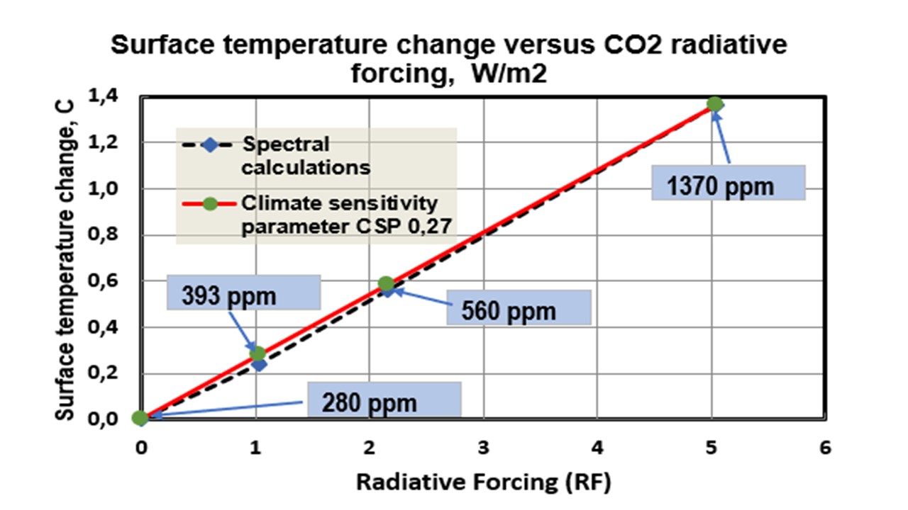
https://wattsupwiththat.com/2017/11/21/new-study-tries-to-link-climate-models-and-climate-data-together-in-a-semi-empirical-climate-model/
The warming effects of CO2 can be summarized like this:
1. RF = 3.12 * ln(CO2/280)
2. dT = 0.27 * RF
3. The residence time of the total CO2 is 55 years and the anthropogenic CO2 is 16 years.
4. The contribution of CO2 in the GH effect is about 13 %.
That’s it.
von Neumann was criticizing economists and mathematicians who tried to model relationships by starting with a large number of variables and then dropped the variables that were not statistically significant from their models. This practice is now become common in data analytics (big data). Unfortunately, from a statistical theory perspective, the identified relationships cannot be distinguished from pure coincidence in a particular data set.
Drawing an elephant with four complex parameters by Jurgen Mayer et al., Khaled Khairy, and Jonathon Howard, Am. J. Phys. 78, 648 (2010), DOI:10.1119/1.3254017.”
http://2.bp.blogspot.com/-CkKUPo04Zw0/VNyeHnv0zuI/AAAAAAAABq8/2BiVrFHTO2Q/s1600/Untitled.jpg

Thanks, that link is a keeper.
Yep . A lot depends on your basis functions . And it helps that 1 complex = 2 real .
Thats right.
Another example is Fourier analysis. Fourier synthesis can reproduce complex time series. Without having predictive capabilities.
Exponential curve fitting: http://www.davdata.nl/math/expfitting.html
Polynomial curve fitting: http://www.davdata.nl/math/graphxl.html
all freeware.
I first heard that Carbon Dioxide’s ability to create heat was a Logarithmic Curve about ten years ago.
Interesting the article above.
It isn’t clear that there is anything to be learnt from this. Apart from the obvious fact that there is a unique nth order polynomial passing through any set of n+1 points which is all the author seems to have shown. A more useful graph would be to look at the difference between the polynomial and the log curve for CO2 values greater than 1400. It is then clear that they diverge very quickly. For example if C is 2500 then 3.12*ln(C/280) =6.8
while the polynomial fit gives 22.8. It is then clear which curve is a better fit to the physics.
There is no need for the time being in the planet like Earth to create these kind of relationship for the CO2 concentrations. We simply have not enough fossil fuel to make it happen.
Who said that fossil fuel is the source of the CO2?
Look back in history… it’s pretty clear that climate changes result in massive CO2 changes. 🙂
“I carried out my calculations using the temperature, pressure, humidity, and GH gas concentration profiles of the average global atmosphere and the surface temperature of 15 ⁰C utilizing the LBL method.”
So your calculations are for this specific assumption and nothing else?
Using 15 ⁰C, an arithmetical average is bogus except in the case where temps are actually all equal. Any body with hot bits and balancing cold bits will radiate a given amount at a LOWER average temp than if temps were uniform. Rotation makes a difference too.
Tom in Florida. I do not know what you have expected me to do. I have shown the results of the reproduction of the equation, which shows the RF value dependency on the CO2 concentration. If you have any knowledge about the climate science, it is the most important physical relationship between the global warming and the increasing CO2 concentration. You need only the value of a climate sensitivity parameter and oops, you can calculate by yourself, what is the climate sensitivity value.
curve fitting is guessing … not theory –> data —> proof … i.e. its not science its a circle jerk …
Here we come. It looks like that you have not understood at all, what is the content of a blog. When you see a curve fitting = rubbish.
Here’s the problem with polynomial fitting…
If I extend the trend line to the next doubling of CO2, the polynomial skyrockets. There’s no predictive value.
well that’s just the Elephant lifting its trunk
hockey!
stick.
Yup. A polynomial can be good for constructing a calibration curve. But this requires a) data and b) that it is only used within the range of available data. Neither of these apply to the prognostications of climate science catastrophe.
There is no data here at all (or “prognostications”). He calculates forcing using BBM on a standard atmosphere. So there is no issue of “range of available data”. The only reason why he is fitting to four points is that he didn’t want to calculate more.
“There is no data here at all”
Sort of like most of the planet when it comes to inventing the mythical ‘average global temperature.
Yup. I’ve used instruments with calibration curves that are 7th order polynomials. Just need very precise measurements of calibration standards and high resolution readings from the instrument being calibrated. But in most cases the coefficients of 4th and higher order terms are 10^-5 or smaller and of no practical importance relative to other uncertainties of measurement. In almost any lab, we’d be very happy to be able to confidently claim an uncertainty of +/- 1% or better for measuring anything. Where much lower uncertainty is necessary, it becomes a matter of whether the cost is justified. e.g. A NIST certified primary reference standard can cost 10 to 100 times a commercial secondary standard reference.
Au contraire, Mr Stokes. This is the sort of thing that global warming catastrophists, and environmentalists at large, indulge in all the time. It is the bread and butter of their existence. Demonstrate, say, a clear relationship between human mortality and increased temperature over the range 40 to 50 Celsius and then claim rising temperatures are bad for humans at some other temperature outside the range.
Sure, that is an example that few people will fall for, but it sums up much of the thinking. They just don’t usually couch their most outrageous assertions in mathematics or a form simple enough for the unwary to immediately spot it and laugh it off. But a mathematical curve fit still expresses a thought or hypothesis.
To Nick Stokes.
This is interesting. You write: “He calculates forcing using BBM on a standard atmosphere. So there is no issue of “range of available data”.”
I guess you did read carefully enough the content of the blog. It was not me using BBM method. It was Myhre et all. I used the line-by-line (LBL) method.
Dr Ollila
“I used the line-by-line (LBL) method.”
Apologies for that. I read the sentence “The data points RF versus CO2 concentrations have been calculated using the BBM (Broad Band Model) climate model” when looking up what you had used, and didn’t read on.
And you fully deserve what you get.
Here the third order polynomial is almost surely overfit. That is to say a second order fit would provide an adequate representation of the data. Adding the third term to the fit results in an improvement, but the improvement is not statistically significant. {wee p-values again!} Therefor, the data is said to be overfit. It is well known that extrapolating (projection, in ClimateScience) overfit polynomials leads to disaster at a geometrically increasing rate.
Everybody maintains that polynomials are no good for making predictions.
In fact, polynomials are great for making scary predictions.
{As the blue line shows, choosing a mathematical function which properly represents the underlying physical phenomena, gets you closer to the truth, faster. But that is science, and we do not do things like that in ClimateScience!}.
“the improvement is not statistically significant”
Statistical tests are pointless here. You can calculate whatever points you like.
@ur momisugly Nick Stokes:
Interesting point.
I am an empirical type since way back. Whenever I see data graphed, I instantly think measurement data. That is really all I have ever worked with. Back in the day, people would construct theoretical curves to explore some phenomena, of course. Often these curves would often be calculated point by point. But we never generated experimental data sets via calculation alone.
This whole modern idea of calculating a data set and then treating it as measurement data sometimes gets confusing to me. I perhaps sometimes lose sight of which is which.
On the other hand:
1) You have a set of data points. It does not matter how the data was obtained; calculated, measurement, tooth fairy, whatever.
2) You select a model; linear, polynomial, logarithmic, and so on.
3) A statistical test informs how well your model represents the data set. complete with wee p-values.
“A statistical test informs how well your model represents the data set”
If there were a dataset. But it actually tells you only about the points “you chose to calculate”. There is no underlying randomness. You might as well to a p-test for however well the log function is approximated by a truncated Taylor series.
Polynomials are great for making “spectacular” predictions in either or both directions… 😉
“A statistical test informs how well your model represents the data set”
All that is being tested here is the difference between 2 deterministic curves. The test is just some measure of difference eg sum squares. This head post is really just showing show well the stated polynomial approximates the log. That is just ordinary stuff about functions. Here is the continuous plot:
“There’s no predictive value.”
There is no prediction here. It is just a relation between calculated values and a simplifying curve. 1400 ppm is not an observed value. If you want to know the value at 2500 ppm, you don’t have to wait; you can calculate it in the same way.
True that.
Nick
OT.
You showed a graph comparing GHCNM adjusted/unadjusted the other day. Can I ask if you calculated individual anomaly baselines for the two sets or if you used one common? If one common, was QCU or QCA used as the baseline?
Thanks
MrZ,
I have described the process here. It is a least squares method, which doesn’t require data in any particular interval. BEST subsequently adopted a similar method. Once the anomalies have yielded a spatial average, one can subtract the global average for any particular interval so the mean will be zero there. I do that with 1961-90.
This is done separately for adjusted and unadjusted. But both are then normalised to 1961-90.
Nick,
Impressive!!!
Will keep me busy for a while 😎
Simple comparison AVG(tavg.qca – tavg.qcu) using data with OK qcflag AND values>-99.99C gives -0.3C during 1930s and close to -0C since 2000.
I have also noticed that tavg.qcu != (tmin.qcu+tmax.qcu)/2 for 5% of the OK records
We talked about anomaly as linear… Interesting to group by station’s monthly baseline temp to see how temps deviates from that baseline depending on warmer or colder years. Dramatic for cold baselines and almost flat for warm baselines.
Don’t want to hijack this thread so I’ll post comments on the site you linked.
Value to be predicted for 1400 or 2500 PPM? I see a strawman (polynomial) being constructed as a comparison to logarithmic, with the strawman getting drawn by some as an elephant, or an elephant lifting its trunk. And, I see this as a distraction from another elephant, the one in the room where we are. I suspect a game of distraction from seeing elephants in the room, by someone who I have seen as finding less effect of global atmospheric CO2 before – by claiming in a comment in a previous WUWT article that outgoing longwave IR gets completely absorbed by CO2 before getting past 1 km above the surface, even though in an earlier comment in that same WUWT article someone with his name published spectral absorption curves for the total thickness of the average global atmosphere for some wavelengths that matter having absorption by CO2 being notably between 0 and 100 % and all other named greenhouse gases having absorption well below 100%.
I refer to the reply before. There is no need for the concentrations above 1300 ppm. Simple like that.
The purpose of trend line is to demonstrate the mathematical relationship between two variables for the purpose of interpolating and/or extrapolating values. A polynomial function can’t be used to extrapolate values.
With climate data, the primary purpose of trend line functions is extrapolation.
I just repeat it once again. For the next 200 years at least, it is good enough to know the RF and warming effects of the CO2 concentrations up to about 1400 ppm. Going further than that is purely academic exercise. We should be able to know what is going to happen during this century. And it is not a problem to calculate the effects up to 10 000 ppm. Actually I have calcualted but I have not shown the results, because they have no meaning.
aveollila February 22, 2018 at 11:13 pm:
“I refer to the reply before. There is no need for the concentrations above 1300 ppm. Simple like that.”
The past history of the Earth had atmospheric CO2 concentration higher than 1300 PPM and somewhat known with global temperature somewhat known, although the accuracy and precision of global temperature and global atmospheric CO2 concentration get a little lower as one explores into the past? These are known enough to have been raised as argument points in WUWT for climate sensitivity to CO2 change being low and for atmospheric CO2 to be known to lag global temperature from 400,000-plus years ago (as a positive feedback mechanism) until humans started bigtime mining and burning of fossil fuels, that were mostly formed more than 100 million years ago. From at least 400,000 years ago to 150 years ago, the sum of carbon (including in carbon compounds) in the sum of the atmosphere, hydrosphere and biosphere was fairly constant. Global temperature change initiated by a cause other than atmospheric CO2 change often got reinforced by positive feedbacks from surface albedo change (especially in the middle-upper northern latitudes in the past few million years, more so when northern continental ice sheets were at least intermittently unstable while getting as far south as 40 degrees north), secondarily due to balance between oceanic and atmopspheric CO2 being a lesser positive feedback.
Nowadays, the effect of increasing atmospheric CO2 has different effects than it did in about 398,500 of the past 400,000 years, because most of the atmospheric CO2 increase is not from global warming since the Little Ice Age, not even according to the NASA GISS version of how much global temperature increased since the Industrial Revolution. From at least 400,000 to around 150 years ago, global temperature change (initiated by something other than CO2 change, such as one or two of the Milankovitch cycles) was reinforced by a lagging transfer of CO2 to/from the atmosphere from/to the oceans. Nowadays, we have CO2 increasing in the atmosphere much more than according to the global temperature increase typically associated with such an amount of CO2 increase. Also nowadays, carbon in the carbon cycle(s) is increasing in all of the atmosphere, hydrosphere and biosphere, and usual from 400,000 to 150 years ago was for carbon in these to get shifted around in response to and to reinforce a temperature change, as opposed to the sum of carbon in the atmsophere, hydrosphere and biosphesre getting a sudden upward trend after the Industrial Revolution due to transfer of carbon from the lithosphere to the sum of the atmosphere, hydrosphere and biosphere.
Prof Ollila,
Your calculations may be of interest to geologists studying the issue of Snowball Earth.
Snowball Winter in Finland?
The recent satellite picture of a snow covered Finland is spectacular.
I see that the forecast for Porvoo continues to be for cold weather this week.
Please stop sending us your global warming!
David. I simply repeat the point given already in my comments. The maximum value of 1370 ppm is good enough. We have not enough fossil fuel reserves to increase the CO2 concentration above 1000 ppm. So in this case this kind of extrapolation is a theoretical exercise only.
Fossil fuel “reserves” are irrelevant to how high the atmospheric CO2 concentration could be. Without burning any fossil fuels, CO2 levels have routinely exceeded 1,000 ppm over the Phanerozoic Eon. Less than 1,000 ppm has been the exception rather than the rule.
The purpose of developing a mathematical relationship between CO2 and temperature is to be able to quantify and predict how one variable will affect the other.
In fact, one long term test of the models is which parameter will go wildly out of bounds first: temperature or CO2.
Mr. Pete: CO2 is increasing with global temperature increasing less than according to the “historical” (usual within the last 400,000 years) correlation. I see two factors for this:
1) Global climate sensitivity varies with global temperature, being greater when northern hemisphere continents have higher mobility (advancing or retreating) of year-round sunshine-getting ice/snowpack coverage. I see this as having gotten to positive feedback occasionally to the extent of instability, at times when global temperature was colder than it got during the Little Ice Age. And when global temperature got warmer than that ofd the Medieval Warm Period, global climate sensitivity was lower, due to less surface albedo positive feedback and greater (negative) lapse rate feedback, the negative one on global temperature (a convective one) as opposed to the one on the global lapse rate itself.
2) Historically within the past 400,000 years, atmospheric CO2 concentration generally lagged global (or icy polar continental region) temperature. During the first 399,800 of those years, the sum of carbon/CO2, as in carbon involved in the carbon cycle that I learned from library books and got taught about in school before “global warming” or “greenhouse effect” became political catchphrases, was fairly constant. There was not much formation or burning of “fossil fuels” during that time. And global temperature changes were usually caused by something other than atmospheric concentration of greenhouse gases, such as the Milankovitch Cycles affecting insolation of a range of Arctic and near-Arctic high latitudes and upper-middle latitudes, and arguably northern latitudes as low as around sometimes even a little below 40 degrees north often mattered, for the surface albedo positive feedback. More when the extratropical and “subtropical” (nearly and barely tropical, and “subtropical” gets up to about 40 maybe 41 degrees north according to some definitions as old as around 1980) gets intermittent or occasional snow coverage. Please note that Atlanta GA, Birmington AL, Nashville TN, Dallas and San Antonio and El Paso TX have gotten some notable wintry weather by more than one definition in the past few decades, mostly because historically the weather “has a temper” in the northern temperate (as opposed to temperant) zone.
Back to atmospheric concentration CO2, that was mostly a positive feedback
But we do have access to a vast quantity of limestone.
All that is needed to raise the CO2 concentration above 1000 ppm is to manufacture a great deal of cement!
It sounds to me that the curve fitting argument here is a strawman one. The logarithmic effect of variation of CO2 is not perfectly logarithmic (it must change to linear, probably in a gradual manner, around some point as concentration decreases somewhere below 180 PPMV and I suspect it flattens slightly more than logarithmic does due to saturation effects with increase to past 1000-1200 PPMV), but it is known as better than a strawman (to knock down) for having its behavior being described by a logarithm function.
The logarithmic effect might even be fictional.
https://climateaudit.org/2008/01/07/more-on-the-logarithmic-formula/
However, nature of the greenhouse effect is almost certainly a diminishing returns function, which can be approximated with a logarithmic equation.
Perhaps I misunderstand the thrust of what you are saying.
If you are just talking about “models and the number of parameters”, apologizes in advance.
But if you are in someway defending “Climate Models”, there are an “H” of a lot more parameters and interactions between those parameters than any “Climate Model” could ever hope to project.
I said this some time ago. What “Climate Model” accounts for all of the possibilities?
As for me, I would rather hedge my bets on the idea that most of the scientists are right than make a bet that most of the scientists are wrong and a very few scientists plus lots of the ideologues at Heartland and other think-tanks are right…But, then, that is because I trust the scientific process more than I trust right-wing ideological extremism to provide the best scientific information.
Even though the vast majority of scientists agreeing with it cannot duplicate it, have never tried to duplicate it, and don’t have access to the the full descriptions of what was done to verify it using validated procedures?
But the comparison is also largely miss-stated, as for the most part, it is one side saying we have successfully created a functioning accurate model and it has been “settled science” for over 25 years (despite being wrong when forecasting anything long enough to show statistical significance) vs. a side that says they don’t know enough to make the claims they are making and being able to show basic flaws.
https://doi.org/10.1119/1.3254017
Drawing an elephant with four complex parameters
American Journal of Physics 78, 648 (2010); https://doi.org/10.1119/1.3254017
Jürgen Mayer
Max Planck Institute of Molecular Cell Biology and Genetics, Pfotenhauerstr. 108, 01307 Dresden, Germany
Khaled Khairy
Log(x+a) is given as a Taylor series:
= ln(a) + (x-a) / a – (x-a)2 / 2a2 + (x-a)3 / 3a3 – (x-a)4 / 4a4 + …
The terms rapidly diminish as their power increases. That is why a polynomial can be fitted to a log curve.
“The terms rapidly diminish as their power increases. “
Not very rapidly. The series converges only to x=2*a, and of course very slowly as you get close.
Personally I’d leave creating an elephant to boy and girl elephants but there’s no accounting for human hubris in such matters.
Meanwhile some interesting new material for sediment fans-
https://www.msn.com/en-au/weather/topstories/heavy-rain-in-new-zealand-creates-a-river-of-rocks/vi-BBJt8h5
Someday I will again come across Benoit Mandelbrot’s (quoted?) statement that reality is fractally complex..
I learned that shortly after David. M. Raup (‘Nemesis’ ’Extinction’) encouraged me to pursue an assertion in discussion that extrapolating points on an epistemological map was freighted, not least by the low order of the model.
First, parametres need to have a physical explanation for why the formulae might be right. For example, Grant Foster and Rhamstorf 2011 fitted 4 parametres to the annual temperature value but they had the solar cycle being a negative value, The higher solar irradiance got, the lower temperature that resulted. Obviously, the wrong result and an example of overfitting and or using the wrong input data (they actually used an incorrect solar irradiance dataset on purpose because it made the CO2 parametre look higher).
Secondly, “time” needs to be a factor in any energy flow equation (such as surface temperature). They use emissivity sometime to substitute for this factor but it needs to be way more in depth to accurately represent the trillions upon trillions of molecules of air, surface and water. Time needs to factored in at the pico-second level and hourly level. The “Ocean Lag” is a perfect example of how this can go wrong. Many formula say the Ocean Lag is 100s of years long, others say 30 years and then the climate models actually only use 7 years for the ln(Co2) formula. Complete garbage in other words..
Third, don’t they think they need to actually test this ln(CO2) formula against what has actually happened on Earth, If you try to do this, you find there is ZERO correlation. It doesn’t mean the formula is wrong, it just means that many other factors such as Albedo, must play an even larger part.
Fourth, what about the 99% of other atmospheric molecules. The theory treats them as having no impact at all. What if the atmosphere has 30% Oxygen rather than 21%? What if the atmosphere is 70% CH4 as in 3.5 billion years ago. Is Nitrogen actually an inert gas in a warm atmosphere? Not a chance. Nitrogen is absorbing energy and giving up energy just like every other molecule in the universe.
The situation is just far too complicated for a ln(CO2) formula to be accurate in any way.
“Secondly, “time” needs to be a factor in any energy flow equation (such as surface temperature). ”
Agreed.
Antero Ollila
Thanks for your excellent discussion. The LBL log function fits the physics better.
For how to curve fit an elephant’s trunk see:
Drawing an elephant with four parameters
How to fit an elephant
Source: “Drawing an elephant with four complex parameters” by Jurgen Mayer, Khaled Khairy, and Jonathon Howard, Am. J. Phys. 78, 648 (2010), DOI:10.1119/1.3254017.
Posted: Freeman Dyson, A meeting with Enrico Fermi,
Noble Laureate Freeman Dyson wrote:
Global climate models
1) have far more than five fitted parameters.
2) They try to model multiple weakly coupled non-linear chaotic systems
3) with inadequate data
4) without exhaustive boundary conditions, AND
5) with widely varying economic and energy use scenarios.
Better to recognize the impossibility of making accurate projections and try stochastic modeling, realistic resilience planning etc.
To David L Hagen.
And a funny thing is that the same warming values can be calculated by both the most complicated GCMs and the simplest IPCC’s climate model as I have shown in my earlier blog:
https://wattsupwiththat.com/2017/12/11/on-the-ipcc-climate-model/
The IPCC’s simple model can be used for calculating both the transient and equilibrium climate sensitivity values and all the IPCC’s scenario values for different RCPs. How it is possible? Maybe they do carry out a lot of parameter fittings in GCMs in order to get the same results as by the simple IPCC model.
It must be fun building hypothetical planets with hypothetical climates by modeling. I fail to see any relationship to reality. I can probably tell you more about the climate by stepping outside my door. It is often cold, cloudy and snowy in Alberta in winter. What does your model tell you? Building a model appears like a waste of good minds.
Rockyredneck.
Hereyou find a climate model with a standard error of 0.1 degrees Celsius starting from 1610 when IPCC starts from 1750.
https://wattsupwiththat.com/2017/11/21/new-study-tries-to-link-climate-models-and-climate-data-together-in-a-semi-empirical-climate-model/
IPCC does not want to touch yearlier years because:
a) there has been no temperature variations before 1750, because the CO2 concentration was the same.
b) because IPCC do not cenfess any other contributors than GH gases.
Antero Ollila has transformed the logarithmic data such that all that is required is a linear regression. Then, upon solving this linear equation, we know, a priori, that a four degree polynomial will fit the data, as well.
Where’s Pamela? I would have thought she’d be all over this thread.
Your calc: RF = 3.12 * ln(C/280)
Why not just use pi. 3.1415926537…? an irrational number.
In nature, we find (pi) popping up all over the place.
Besides, rationality left the climate modellers decades ago.
The coefficeint of 3.12 is the result of a curve fitting. You cannot select it. If you do it, your curve will not fit with the data points.