Guest essay by Antero Ollila
The error of the IPCC climate model is about 50% in the present time. There are two things that explain this error:
1) There is no positive water feedback in the climate, and 2) The radiative forcing of carbon dioxide is too strong.
I have developed an alternative theory for global warming (Ref. 1), which I call a Semi Empirical Climate Model (SECM). The SECM combines the major forces which have impacts on the global warming namely Greenhouse Gases (GHG), the Total Solar Irradiance (TSI), the Astronomical Harmonic Resonances (AHR), and the Volcanic Eruptions (VE) according to observational impacts.
Temperature Impacts of Total Solar Irradiance (TSI) Changes
GH gas warming effects cannot explain the temperature changes before 1750 like the Little Ice Age (LIA).
Total Solar Irradiance (TSI) changes caused by activity variations of the Sun seem to correlate well with the temperature changes. The TSI changes have been estimated by applying different proxy methods. Lean (Ref. 2) has used sunspot darkening and facular brightening data. Lean’s paper was selected for publication in Geophysical Research Letters “Top 40” edition and it was rewarded.

Lean has introduced a correlation formula between the decadally averaged proxy temperatures and the TSI:
dT = -200.44 + 0.1466*TSI from 1610 to 2000. In my study the selection of century-scale reference periods for TSI changes are selected carefully so that the AHR effect is zero and the forcings of GH gases are eliminated. The Sun causes the rest of the temperature change. The temperature changes of these reference periods caused by the Sun are 0 ⁰C, 0.24 ⁰C and 0.5 ⁰C, which are relatively great and different enough – also practically the same as found by Lean but the correlation is slightly nonlinear (Ref. 1):
dTs = -457777.75 + 671.93304 * TSI – 0.2465316 * TSI2
Nonlinearity is due to the cloudiness dependency on the TSI. This empirical relationship amplifies the direct TSI effect changes by a factor of 4.2. The amplification is due to the cloud forcing caused by the cloudiness change from 69.45 % in 1630s to 66 % in 2000s. A theory that the Sun activity variations modulate Galactic Cosmic Ray (GCR) flux in the atmosphere has been introduced by Svensmark (Ref. 3), which affect the nucleation process of water vapour into water droplets. The result is that the higher TSI value decreases cloudiness, and in this way, there is an amplification in the original TSI change.
Astronomical Harmonic Resonances (AHR) effects
The AHR theory is based on the harmonic oscillations of about 20 and 60 years in the Sun speed around the solar system barycentre (gravity centre of the solar system) caused by Jupiter and Saturn (Scafetta, Ref. 4). The gravitational forces of Jupiter and Saturn move the barycentre in the area, which has the radius of the Sun. The oscillations cause variations in the amount of dust entering the Earth’s atmosphere (Ermakov et al., Ref. 5). The optical measurement of the Infrared Astronomical Satellite (IRAS) revealed in 1983 that the Earth is embedded in a circumsolar toroid ring of dust, Fig. 2. This dust ring co-rotates around the Sun with Earth and it locates from 0.8 AU to 1.3 AU from the Sun. According to Scafetta’s spectral analysis, the peak-to-through amplitude of temperature changes are 0.3 – 0.35 ⁰C. I have found this amplitude to be about 0.34 ⁰C on the empirical basis during the last 80 years.

The space dust can change the cloudiness through the ionization in the same way as the Galactic Cosmic Rays (GCR) can do, Fig.3.

Because both GCR and AHR influence mechanisms work through the same cloudiness change process, their net effects cannot be calculated directly together. I have proposed a theory that during the maximum Sun activity period in the 2000s the AHR effect is also in maximum and during the lowest Sun activity period during the Little Ice Age (LIA) the AHR effect is zero (Ref. 1).
GH gas warming effects
In SCEM, the effects of CO2 have been calculated using the Equation (2)
dTs = 0.27 * 3.12 * ln(CO2/280) (2)
The details of these calculations can be found in this link: https://wattsupwiththat.com/2017/03/17/on-the-reproducibility-of-the-ipccs-climate-sensitivity/
The warming impacts of other methane and nitrogen oxide are also based on spectral analysis calculations.
The summary of temperature effects
I have depicted the various temperature driving forces and the SCEM model calculated values in Fig. 4. Only two volcanic eruptions are included namely Tambora 1815, Krakatoa 1883.

The reference surface temperature is labelled as T-comp. During the time from 1610 to 1880, the T-comp is an average value of three temperature proxy data sets (Ref. 1). From 1880 to 1969 the average of Budyoko (1969) and Hansen (1981) data has been used. The temperature change from 1969 to 1979 is covered by the GISS-2017 data and thereafter by UAH.
In Fig. 5 is depicted the temperatures from 2016 onward are based on four different scenarios, in which the Sun’s insolation decreases from 0 kW to -3 kW in the following 35 years and the CO2 increases 3 ppm yearly.

The Sun’s activity has been decreasing since the latest solar cycles 23 and 24, and a new two dynamo model of the Sun of Shephard et al. (Ref. 6) predicts that its activity approaches the conditions, where the sunspots disappear almost completely during the next two solar cycles like during the Maunder minimum.
The temperature effects of different mechanisms can be summarized as follows:
| Time | Sun | GHGs | AHR | Volcanoes |
| 1700-1800 | 99.5 | 4.6 | -4.0 | 0.0 |
| 1800-1900 | 70.6 | 21.5 | 17.4 | -9.4 |
| 1900-2000 | 72.5 | 30.4 | -2.9 | 0.0 |
| 2015 | 46.2 | 37.3 | 16.6 | 0.0 |
The GHG effects cannot alone explain the temperature changes starting from the LIA. The known TSI variations have a major role in explaining the warming before 1880. There are two warming periods since 1930 and the cycling AHR effects can explain these periods of 60-year intervals. In 2015 the warming impact of GH gases is 37.3 %, when in the IPCC model it is 97.9 %. The SECM explains the temperature changes from 1630 to 2015 with the standard error of 0.09 ⁰C, and the coefficient of determination r2 being 0.90. The temperature increase according to SCEM from 1880 to 2015 is 0.76 ⁰C distributed between the Sun 0.35 ⁰C, the GHGs 0.28 ⁰C (CO2 0.22 ⁰C), and the AHR 0.13 ⁰C.
References
1. Ollila A. Semi empirical model of global warming including cosmic forces, greenhouse gases, and volcanic eruptions. Phys Sc Int J 2017; 15: 1-14.
2. Lean J. Solar Irradiance Reconstruction, IGBP PAGES/World Data Center for Paleoclimatology Data Contribution Series # 2004-035, NOAA/NGDC Paleoclimatology Program, Boulder CO, USA, 2004.
3. Svensmark H. Influence of cosmic rays on earth’s climate. Ph Rev Let 1998; 81: 5027-5030.
4. Scafetta N. Empirical evidence for a celestial origin of the climate oscillations and its implications. J Atmos Sol-Terr Phy 2010; 72: 951-970.
5. Ermakov V, Okhlopkov V, Stozhkov Y, et al. Influence of cosmic rays and cosmic dust on the atmosphere and Earth’s climate. Bull Russ Acad Sc Ph 2009; 73: 434-436.
6. Shepherd SJ, Zharkov SI and Zharkova VV. Prediction of solar activity from solar background magnetic field variations in cycles 21-23. Astrophys J 2014; 795: 46.
The paper is published in Science Domain International:
Semi Empirical Model of Global Warming Including Cosmic Forces, Greenhouse Gases, and Volcanic Eruptions
Antero Ollila
Department of Civil and Environmental Engineering (Emer.), School of Engineering, Aalto University, Espoo, Finland
In this paper, the author describes a semi empirical climate model (SECM) including the major forces which have impacts on the global warming namely Greenhouse Gases (GHG), the Total Solar Irradiance (TSI), the Astronomical Harmonic Resonances (AHR), and the Volcanic Eruptions (VE). The effects of GHGs have been calculated based on the spectral analysis methods. The GHG effects cannot alone explain the temperature changes starting from the Little Ice Age (LIA). The known TSI variations have a major role in explaining the warming before 1880. There are two warming periods since 1930 and the cycling AHR effects can explain these periods of 60 year intervals. The warming mechanisms of TSI and AHR include the cloudiness changes and these quantitative effects are based on empirical temperature changes. The AHR effects depend on the TSI, because their impact mechanisms are proposed to happen through cloudiness changes and TSI amplification mechanism happen in the same way. Two major volcanic eruptions, which can be detected in the global temperature data, are included. The author has reconstructed the global temperature data from 1630 to 2015 utilizing the published temperature estimates for the period 1600 – 1880, and for the period 1880 – 2015 he has used the two measurement based data sets of the 1970s together with two present data sets. The SECM explains the temperature changes from 1630 to 2015 with the standard error of 0.09°C, and the coefficient of determination r2 being 0.90. The temperature increase according to SCEM from 1880 to 2015 is 0.76°C distributed between the Sun 0.35°C, the GHGs 0.28°C (CO20.22°C), and the AHR 0.13°C. The AHR effects can explain the temperature pause of the 2000s. The scenarios of four different TSI trends from 2015 to 2100 show that the temperature decreases even if the TSI would remain at the present level.
Open access: http://www.sciencedomain.org/download/MTk4MjhAQHBm.pdf
crackers345 November 21, 2017 at 10:10 pm
Again, you seem to misunderstand parameterization. Ohm’s Law ( E = I R ) is an actual physical law, not a parameterization. The same is true of the Ideal Gas Law ( P V = n R T ) and Hooke’s Law (extension is proportional to force).
Here’s a reasonable definition of parameterization from the web:
Note that the “simplified process” is indeed “just made up” by the programmers …
And more to the point, as you can see, parameterization has ABSOLUTELY NOTHING TO DO WITH OHM’S LAW!!! It’s amazing, but sometimes you really, actually don’t understand what you are talking about …
w.
willis commented – “Ohm’s Law ( E = I R ) is an actual physical law, not a parameterization. The same is true of the Ideal Gas Law ( P V = n R T ) and Hooke’s Law (extension is proportional to force).”
Absolutely not.
they are all parametrizations — curve-fits that apply
only in a certain region of their variable space.
V=IR fails outside of certain ranges. So does
hooke’s law. so does the ideal gas law (see, for
example, van der waals equation, a gas equation, also
a parametrization, that tries to improve upon
the ideal gas law).
all of these are “parametrizations” — laws that do not
arise from fundamental, microscopic physics but which
are empirically derived over a certain
region of variable space.
and the parametrizations used in
climate models aren’t just made up out
of the
blue — they come
from studies of the variable
space to which they
pertain.
lots and lots
of papers have done
exactly this.
willis commented – “It’s amazing, but sometimes you really, actually don’t understand what you are talking about”
i’d say right back at you — but
i try to avoid ad homs and stick
to the science
IPCC plays in many cases with two different cards. The Assessment Reports (AR) are not only the literature surveys of the climate change science. An AR also shows the selections of IPCC. As an example, IPCC selected Mann’s temperature study among hundreds of scientific publications to be the correct one or the best one of TAR in 2001. In the later ARs IPCC has been silent about this choice.
It is a fact the IPCC has made selections, which create the conclusion that the global warming is human induced – so called AGW theory. Otherwise there would be no general idea about the reasons of the global warming. This has also been the basis of the Paris Climate agreement.
When we start talking about the climate models, people think that they are those complicated GCMs, which are used for calculating the impacts of increased GH gas concentrations, which are the reasons for warming. United Nations and its organizations running the Climate treaties, has only one scientific muscle and it is IPCC. When the temperature effects are needed like calculating the transient climate sensitivity (TCS) and the temperature effects of RCPs during this century and CO2 concentrations up to 1370, it turns out, that a very simple model has been applied:
dT = CSP*RF, (1)
RF = k * ln(C/280) (2)
where CSP is Climate Sensitivity Parameter, and C is CO2 concentration (ppm). IPCC’s choices have been CSP = 0.5 K/(W/m2) and k = 5.35.
It seems to create strong reactions for some people like Nick Stones, that I call this a IPCC’s model. Even it is simple, it is a model. There is no rule that a simple model should not be called a model. There are many simple models. And why I can call it a “IPCC’s model”? Therefore, that IPCC has used this model in the most important calculations (CS and RCPs), and the equations as well as the parameters are IPCC chosen.
Some questions for those who disagree:
1) Why IPCC uses a lot of effort for calculating and reporting RF values for different factors in global warming? Actually, for all the factors affecting the global warming according to IPCC.
2) What is the purpose of summarizing the RF values of different factors, if the sum cannot be used for calculating a temperature effect?
3) Why it turns out that in the end IPCC utilizes its model for calculating the real-world temperature effects? Why IPCC seem to hide this calculation basis (IPCC model), even though it can be easily figured out?
4) Why IPCC has reported the total RF value of 2.34 W/m2 in 2011 but has not used its model for calculating the temperature effect? This is my guess: The error is too great if compared to the measured temperatures. In the cases of CS and RCP, there is no such a problem, because there are no measurement values to be referred to.
@aveollila, Additional evidence for what you say is the vaunted “450 Scenario” by which IPCC asserts that keeping atmospheric CO2 below 450 ppm limits further warming to 2C (1.15C on top of 0.85C). Clearly IPCC posits a simple mathematical relationship between measured CO2 and estimates of GMT. They further claim that all of the rise in CO2 comes from exactly 50% of fossil fuel emissions retained in the atmosphere. So now the objective is clear: Only an additional 100 ppm of fossil fuel emissions is allowed.
Fighting Climate Change is deceptively simple, isn’t it? sarc/off
Oh, the last step involves 1 ppm CO2 = 2.12 Gt carbon or 7.76 Gt CO2. From there budgets are calculated for every nation.
ave commented – “It seems to create strong reactions for some people like Nick Stones, that I call this a IPCC’s model. Even it is simple, it is a model.”
this is definitely not “ipcc’s model” – it goes
back to at least arrhenius in 1896.
it’s also quite a good parametrization, at the
levels of co2 we’re experiencing….
but still, i don’t think serious climate models use this
equation. instead they solve the schwarzschild
equations at each level in their gridded atmosphere –
or call on a subroutine that has already done that.
Seems to me that this paper makes a reasonable attempt to explain the global temperature history by reference to plausible factors that probably affect it. There are obvious issues in establishing that history but that does not invalidate the conclusions. My expectation is that recorded temperatures will continue to rise as the past cools, but that will be accompanied by severe frosts and heavy snowfalls. It is obvious to anyone with a passing acquaintance with human history and who follows this issue that CO2 cannot be the main influence on climate, but must have some effect. It is only one factor in the mix though and any sensible attempt to quantify this should be applauded – though personally I have no way of determining whether this paper ascribes correct values. However CAGW has become so politicized and part of so many peoples’ belief system I don’t expect this paper or others like it to get “a fair hearing” more generally.
Certainly not all wrong.
We know to a reasonable degree of confidence what drives global temperature and it is almost entirely natural and has an INSIGNIFICANT causative relationship from increasing atm. CO2:
– in sub-decadal and decadal time frames, the primary driver of global temperature is Pacific Ocean natural cycles, moderated by occasional cooling from major (century-scale) volcanoes;
– in multi-decadal to multi-century time frames, the primary cause is solar activity;
– in the very long term, the primary cause is planetary cycles.
Reference by Nir Shaviv:
http://www.sciencebits.com/CosmicRaysClimate
Does anyone have a non-paywalled copy of reference 5?
I can only find and abstract and first page here https://link.springer.com/article/10.3103/S1062873809030411
Antero Ollila’s “Semi-Empirical Climate Model” deserves a lot of credit for taking into account the influence of variations in solar irradiance, and the dust concentrations due to the changes in the center of gravity of the solar system due to motions of Jupiter and Saturn, on temperatures on Earth. Ollila’s model predicts that the Earth’s temperature will probably decline between now and 2040 due to the dust effects, even if solar irradiance does not decrease between now and then. Most other climate models cited by the IPCC do not even consider “Astronomical Harmonic Resonances”.
Ollila’s model still has the weakness of using an Arrhenius-type model for the temperature change due to greenhouse gases, of the form dT = K ln (C/Co). Ollila’s Equation 2 sets K = 0.8424 and Co = 280, which results in less predicted temperature change than the IPCC model (from Ollila’s message of 9:31 PM) of K = 2.675, so that Ollila’s estimate of the effect of greenhouse gases is only about 31.5% of that by the IPCC.
The problem here is the form of the greenhouse-gas effect equation, even if its coefficient is only about 1/3 of that used by the IPCC. In order to model the effect of IR re-radiation from the Earth’s surface being absorbed by gases, the necessary starting point is the Beer-Lambert equation,
dI/dz = -aC (Eq. 3)
where I = intensity of transmitted light (at a given frequency or wavelength)
z = altitude above the earth
a = absorption coefficient (at a given frequency or wavelength)
C = concentration of absorbing gas
If the concentration does not change with altitude, the above equation can be integrated to give
I(z) = Io exp (-aCz) (Eq. 4)
where Io is the intensity of the emitted radiation at the earth’s surface, as a function of frequency according to the Planck distribution. The energy absorbed by the atmosphere is the surface intensity minus the transmitted intensity, or
E(absorbed) (z) = A[Io – I(z)] = AIo [1 – exp(-aCz)] (Eq. 5)
where A represents an element of area of the Earth’s surface.
Equation 5 is somewhat simplified, because in reality the concentration of any gas in the atmosphere (in molecules per m3) decreases with altitude, according to the ideal-gas law and the lapse rate. In order to calculate the total energy absorption, Equation 5 would have to be integrated over the IR spectrum of frequencies, with the absorption coefficient a varying with frequency.
But the form of Equation 5, which is based on the well-established Beer-Lambert law, shows that the energy that can be absorbed by greenhouse gases is bounded, with an absolute maximum of AIo. The IPCC equation dT = K ln (C/Co) has no intrinsic upper bound, except for the possibility that the Earth’s atmosphere becomes pure CO2 and C = 1,000,000 ppm, and the temperature increase would be about 8.18 times the coefficient K (or if K = 2.675, the temperature increase would be 21.9 degrees C).
Equation 5 also shows that the energy effect for each doubling of CO2 concentrations decreases. For example, if aCz = 2.0 for a given frequency at current CO2 concentrations, the absorbed energy is about 0.8647 * AIo. Doubling the concentration to aCz = 4.0 results in an absorbed energy of 0.9817 AIo, an increase of 0.117 AIo. Doubling the concentration again to aCz = 8.0 results in an absorbed energy of 0.9997 * AIo, or an increase of only 0.018 AIo. This demonstrates the “saturation” effect, where most of the available energy is already absorbed at current concentrations (or by water vapor), and little additional energy is available to be absorbed by higher concentrations of greenhouse gases.
Antero Ollila’s “Semi-Empirical Climate Model” represents a vast improvement over the IPCC climate models, by taking into account fluctuations in solar irradiance and dust effects of the Astronomical Harmonic Resonance.
It could be made even more robust (and more accurate) by incorporating a model for infrared absorption by greenhouse gases based on the Beer-Lambert absorption law (with appropriate adjustments for atmospheric pressure and temperature as a function of altitude), integrated over the infrared spectrum, and consideration of IR absorption by water vapor (which contributes to the saturation effect and reduces the net influence of increasing CO2 concentrations).
Steve Zell. Some years ago I started also from the simple relationship of LW absorption according to Beer-Lambert law. I learned that this law is applicable for a very simple situation and for very low concentration of one gas only. The atmospheric conditions with several GH gases makes the situation so demanding that the only way is to apply spectral calculations. In figure below, one can see that the temperature effect of CO2 follows the logarithmic relationship and it is faraway from Beer-Lambert conditions. The conditions of CH4 and N2O are pretty close to Beer-Lambert conditions except that there is water, which is competing with these molecules about the absorption of LW radiation.

dTs = -457777.75 + 671.93304 * TSI – 0.2465316 * TSI2
It’s pretty silly to carry that many significant figures.
Please be sure to give us regular updates, decadally perhaps, showing fit of the model projections to the accumulating out of sample data. Lots of models of diverse kinds have been published, and I am following (sort of) the updates as new data become available.
It may look like pretty silly but the equation is only slighty nonlinear and that is the explanation for big number and decimals.
Here is a simple “model” which ,I think,produces probably successful forecasts.
1. There are obvious periodicities in the temperature record and in the solar activity proxies.
2. At this time, nearly all of the temperature variability can be captured by convolving the 60 year and millennial cycles.
3 .
Fig.3 Reconstruction of the extra-tropical NH mean temperature Christiansen and Ljungqvist 2012. (9) (The red line is the 50 year moving average.)
This Fig 3 from
http://climatesense-norpag.blogspot.com/2017/02/the-coming-cooling-usefully-accurate_17.html
provides the most useful basis for discussion
4.The most useful Solar “activity” driver data is below
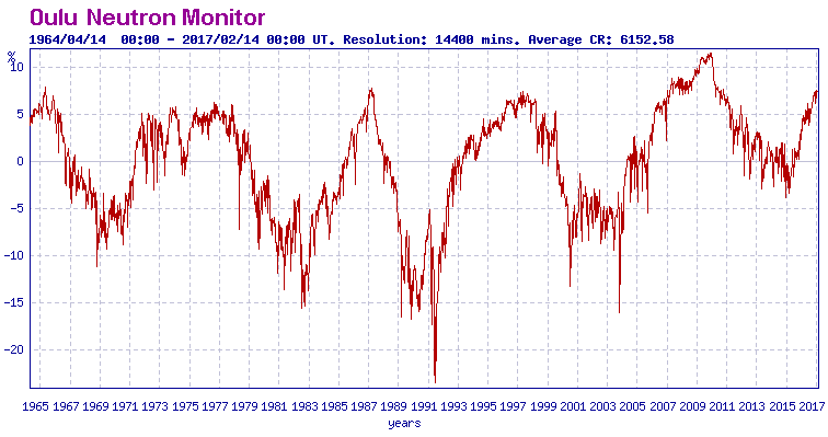
Fig. 10 Oulu Neutron Monitor data (27)
5.The current trends relative to the millennial cycle are shown .below. The millennial cycle peaked at about 2003/4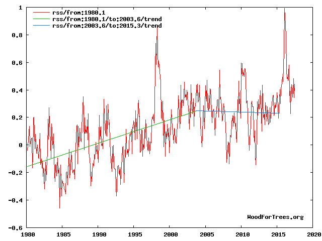
Fig 4. RSS trends showing the millennial cycle temperature peak at about 2003 (14)
Figure 4 illustrates the working hypothesis that for this RSS time series the peak of the Millennial cycle, a very important “golden spike”, can be designated at 2003/4
The RSS cooling trend in Fig. 4 was truncated at 2015.3 , because it makes no sense to start or end the analysis of a time series in the middle of major ENSO events which create ephemeral deviations from the longer term trends. By the end of August 2016, the strong El Nino temperature anomaly had declined rapidly. The cooling trend is likely to be fully restored by the end of 2019.
6..This “golden spike”correlates with the solar activity peak (neutron low) at about 1991 in Fig 10 above. There is a 12 year +/- delay between the solar driver peak and the temperature peak because of the thermal inertia of the oceans.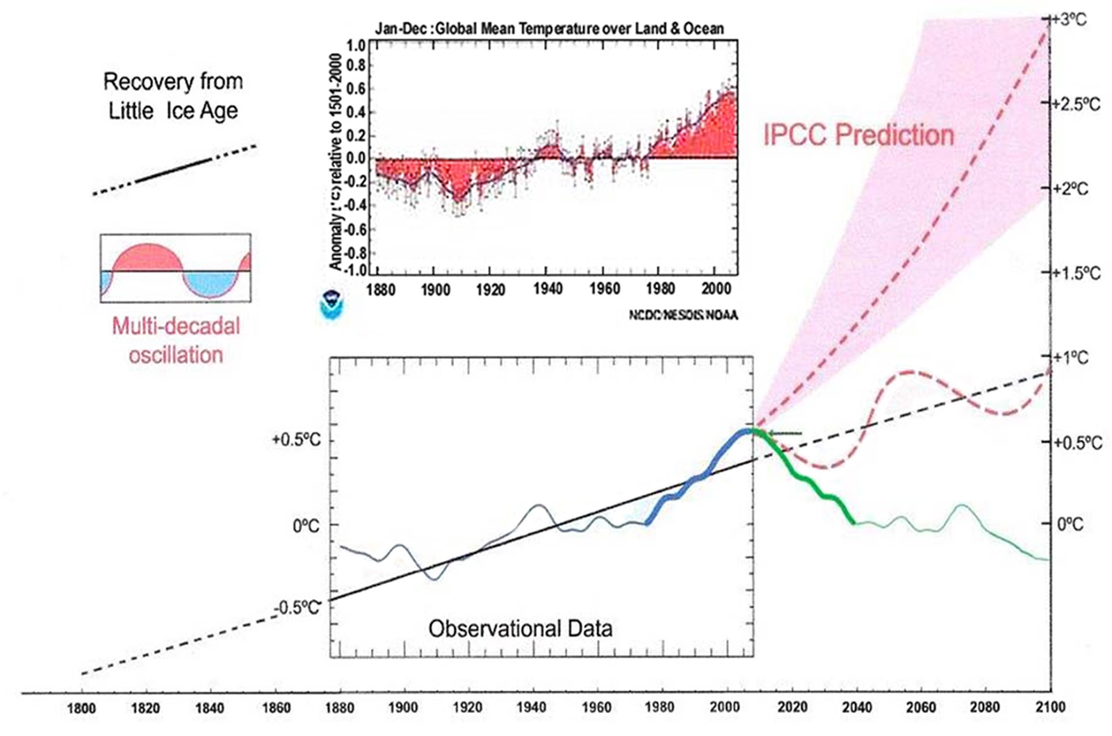
7 Forecasts to 2100 are given below
Fig. 12. Comparative Temperature Forecasts to 2100.
Fig. 12 compares the IPCC forecast with the Akasofu (31) forecast (red harmonic) and with the simple and most reasonable working hypothesis of this paper (green line) that the “Golden Spike” temperature peak at about 2003 is the most recent peak in the millennial cycle. Akasofu forecasts a further temperature increase to 2100 to be 0.5°C ± 0.2C, rather than 4.0 C +/- 2.0C predicted by the IPCC. but this interpretation ignores the Millennial inflexion point at 2004. Fig. 12 shows that the well documented 60-year temperature cycle coincidentally also peaks at about 2003.Looking at the shorter 60+/- year wavelength modulation of the millennial trend, the most straightforward hypothesis is that the cooling trends from 2003 forward will simply be a mirror image of the recent rising trends. This is illustrated by the green curve in Fig. 12, which shows cooling until 2038, slight warming to 2073 and then cooling to the end of the century, by which time almost all of the 20th century warming will have been reversed.
The establishment climate scientists made a schoolboy error of scientific judgement by projecting trends straight ahead across the millennial peak turning point. The whole UNFCC circus which has led to the misuse of trillions of dollars is based on the ensuing delusionary projections of warming.
The latest Unscientific American has a piece from Kate Marvel from the Columbia University Anthropogenic Warming support group discussing clouds. Fig 11 from the paper linked above gives a neat example of the warming peak and inflection point seen in the cloud cover and global temperature.
I have been for many years, why there is no cloudess data after 2010. Has anybody any information, why we do not have this data?
Not sure what that means or how the figure was arrived at. I don’t think we are told, are we?
I only have access to the surface model data via KNMI: https://climexp.knmi.nl/start.cgi
There are dozens of CMIP5 surface models (or variants) for each ‘pathway’, or CO2 emission scenario. The KNMI site allows you to download the ‘mean’ for each scenario, to save on the leg work. As far as the surface data are concerned, it’s fair to say that, while the models are generally running warmer than the observations, the difference isn’t huge.
It depends how you smooth things out, but if you just compare monthly or annual values, then there have been months/years recently when observations have been running warmer than the mean of the model outputs; even in the highest CO2 emissions scenario – 8.5.
If yo smooth it out by a few years, capturing the slightly cooler period around 2012, then the models are running a bit warmer than the observations; but not by much.
The description of the calculation is somewhere in former replies.
I think that I saw a comment that it is not a proper procedure to compare the Climate Sensitivity (CS) results of the IPCC’s simple model (as I call it) and the results of GCMs. I think that according to this comment, CS should be used for diagnosis only. For what diagnosis??
It is not so. The artificial specification of CS (doubling the CO2 concentration from 280 to 560 ppm) has been created just for easy comparisons of different climate models. It makes also a lot of sense, because this concentration change is so great that the differences between the models come clearly out.
I have shown that the IPCC’s simple model gives (1.85 degrees) practically the same CS value as the official figure of IPCC, which is 1.9 C ± 0.15 C, and which is based on GCMs. If the results of two models give the same CS, then the science behind the calculations is the same. Simple like that.
It seems to be a great surprise that the IPCC’s simple model works like this and the warming calculations of IPCC for RCP scenarios are also based on this model as well as the baseline scenario calculations of the Paris Climate Agreement.
Some words about the simple model of IPCC, which is
dT = CSP*RF, (1)
RF = k * ln(C/280) (2)
where CSP is Climate Sensitivity Parameter, and C is CO2 concentration (ppm). IPCC’s choices have been CSP = 0.5 K/(W/m2) and k = 5.35 and my choices are CSP = 0.27 and k = 3.12.
So, I think that the form of the model is correct. It is question about very small changes in the outgoing LW radiation. For example, the CO2 increase form 280 ppm to 560 ppm decreases the outgoing LW radiation by 2.29 W/m2 in clear sky conditions. This decrease is compensated by the elevated surface temperature of 0.69 degrees.
This change can be compared to the total radiation, which is about 260 W/2. The change is about 0.9 % only. I am familiar with the creation of process dynamic models. They are all based on the linearization around the operating point. This situation is very similar. The changes are so small that the simple linear models are applicable. The complicated GCMs are needed to calculate three dimensional changes but the global result is the same as by the simple model.
“CSP is Climate Sensitivity Parameter”
CSP is the equilibrium CSP. It tells what the notional increase in T would be, after abrupt change RF, when everything has settled down, which would take centruies. That is why more elaborate definitions of transient sensitivity are devised. But they have conditions.
Here is what Sec 6.1.1 of the TAR says about it, including the tangential reference to old-time use of 0.5 (my bold)
The CSP value of 0.5 is used for calculating the TCS values, which means that the only positive feedback is water feedback: TCS =0.5*3.7 = 1.85 degrees. The ECS according to AR5 is between 1.5 to 4.5 C which means an average value of 3.0 C. In Table 9.5 of AR5 has been tabulated the key figures of 30 GCMs and the average value of these 30 GCMs is 3.2 C. When using the simple model of IPCC, the corresponding CSP-values are 0.81 and 0.87. In this Table 9.5 is also tabulated the average CSP values of 30 GCMs for ECS and it is 1.0.
Roughly we can say that the ECS can be calculated by multiplying TCS by 2. The ECS values are highly theoretical, because IPCC itself does not use it for calculating real-world values: RCP warming values during this century are calculated using the CSP value of 0.5.
“The CSP value of 0.5 is used for calculating the TCS values”
This is all hopeless if you don’t have a source for the 0.5 number. If it’s the number referred to in TAR 6.1.1, it is explicitly ECS. You can’t just say we’ll call it TCS and use the ECS number. There are different definitions of TCS, none applicable here.
First off, as the author admits, this is an exercise in curve fitting. He has four different curve fits, which if I’ve counted correctly have no less than nine! tunable parameters. With that many parameters, it would be surprising if he could NOT fit the data. I refer the reader to Freeman Dyson’s comments on tunable parameters for the reasons why multi-parameter fits are such a bad idea..
Next, the author seems unaware that one way to test such parameterized fits is to divide the data in half, and run the fitting procedure on just the first half separately. Then, using those parameters, see how well that emulates the second half of the data.
Then repeat that in reverse order, running the fit on the second half and using that to backcast the first half.
Since the author hasn’t reported the results of such a test, I fear that his results have no meaning. Seriously, folks, if you can’t fit that curve with four equations using nine tunable parameters, you need to turn in your credentials on the way out … what he has done is a trivial exercise.
w.
I expected that this kind of comments will emerge. I just remind that the RF equation of Myhre et al. is a result of curve fitting and the result is a logarithmic relationship between the CO2 concentration and the RF value. In this equation there is only one parameter (5.35). I have done the same thing and my value for the parameter is 3.12. So,I know what I am talking about.
Hansen et al. have also developed an equation for the same purpose and they selected a polynomial expression having together 5 parameters. According to Willis, the model of Hansen et al. is just lousy science because of the number of parameters. The truth is that the number of parameters have nothing to do, which model is the best. It is just a question of curve fitting. Of course, a simple model is nice, and it is easy to use. The decisive thing in the end is this: Are the scientific calculations correct in calculating each pair of data points for curve fitting. The number of parameters have no role in this sense.
Yes, I have used curve fitting in all four cases: The Sun effect is pure empirical equation (and so is the equation of gravity, by the way). I could have used the theoretical values of Scafetta for AHR but I preferred the empirical value (one parameter), volcano effects are empirical, and the eggects of GH gases are theoretical in the same way as in the case of IPCC.
aveollila November 22, 2017 at 12:32 pm Edit
There is a solid physical basis for the claim that the relationship between concentration and forcing is logarithmic. Your work has absolutely no such basis.
James Hansen??? You are putting up James Hansen’s work as an ideal?
Get serious. Hansen is a wild alarmist whose work is a scientific joke.
I begin to despair. What you have done is a curve fitting exercise with a large number of parameters. You seem surprised that you’ve gotten a good fit, but with nine parameter that is no surprise at all. It would only be surprising if you couldn’t fit the data, given the head start.
I detailed above how you should have tested the results.
The fact that you either have not done the tests or have not reported them clearly indicates that you are out of your depth. Come back when you have done the tests and report the results, and we’ll take it from there.
w.
Willis Eschenbach commented – “James Hansen??? You are putting up James Hansen’s work as an ideal?
Get serious. Hansen is a wild alarmist whose work is a scientific joke.”
hansen is and will al-
ways be a legend in climate science.
his work was groundbreaking and advanced
the field more
than anyone since manabe, and his
public warnings even
more than that.
when the history of 20th
Cen climate science is fully written,
JHansen will easily
be a top 10 player.
Crackers,
Please state the “groundbreaking” contributions which you imagine Hansen to have made to “climate science”. Thanks.
https://en.wikipedia.org/wiki/James_Hansen#Research_and_publications
https://en.wikipedia.org/wiki/James_Hansen#Analysis_of_climate_change_causation
https://en.wikipedia.org/wiki/James_Hansen#Climate_change_activism
Hansen led the effort to
calculate a rigorous GMST.
His 1988 congressional
testimony changed the
landscape of AGW. (“global
warming has begun)
his 1981
paper in Science was
and will always be
a masterpiece.
I have been criticized that the so-called IPCC’s simple climate model cannot be used for calculating the temperature value for the year 2016. If this model cannot be used, what model can be used and what is the temperature change value for 2016? If a climate model cannot be used for calculating the warming value for a certain year, is it a model at all? It looks like that there is a mysterious climate model, which can be used for calculating temperature increase after 100 years, but nobody knows what is that model and what is more: you should not call it “a IPCC’s climate model”.
I just remind you once more: The warming impacts of RCPs and the Paris climate agreement are based on the IPCC’s science. I have shown in detail, what is this science. Those who criticize my evidences, have not shown any signs about the alternative ways of calculations.
the ipcc doesn’t make
models, they assess
them. and they do that for
many more than one. there is
no “ipcc climate model.”
I don’t see what Scafetta’s 59.6yr Saturn-Jupiter tri-synodic period has to do with an observed AMO envelope of 65-69yrs?
It has nothing to do with it … but that’s never stopped them before and won’t stop them now.
w.
How does one link incomplete and grossly adjusted data to a model that does not represent the climate system?
Climate models have a lot of warming tuned in from hindcast.
“Climate models have a lot of warming tuned in from hindcast.”
how so, exactly?
A science teacher of mine one explained entropy: “If you add a drop of wine to a gallon of sewage you get sewage. If you add a drop of sewage to a gallon of wine you get sewage.”
The models don’t work. You cannot ‘rescue’ them by blending them with data.