Guest Post by Willis Eschenbach
Over at Dr. Curry’s excellent website, she’s discussing the Red and Blue Team approach. If I ran the zoo and could re-examine the climate question, I’d want to look at what I see as the central misunderstanding in the current theory of climate.
This is the mistaken idea that changes in global temperature are a linear function of changes in the top-of-atmosphere (TOA) radiation balance (usually called “forcing”).
As evidence of the centrality of this misunderstanding, I offer the fact that the climate model output global surface temperature can be emulated to great accuracy as a lagged linear transformation of the forcings. This means that in the models, everything but the forcing cancels out and the temperature is a function of the forcings and very little else. In addition, the paper laying out those claimed mathematical underpinnings is one of the more highly-cited papers in the field.
To me, this idea that the hugely complex climate system has a secret control knob with a linear and predictable response is hugely improbable on the face of it. Complex natural systems have a whole host of internal feedbacks and mechanisms that make them act in unpredictable ways. I know of no complex natural system which has anything equivalent to that.
But that’s just one of the objections to the idea that temperature slavishly follows forcing. In my post called “The Cold Equations” I discussed the rickety mathematical underpinnings of this idea. And in “The TAO That Can Be Spoken” I showed that there are times when TOA forcing increases, but the temperature decreases.
Recently I’ve been looking at what the CERES data can tell us about the question of forcing and temperature. We can look at the relationship in a couple of ways, as a time series or a long-term average. I’ll look at both. Let me start by showing how the top-of-atmosphere (TOA) radiation imbalance varies over time. Figure 1 shows three things—the raw TOA forcing data, the seasonal component of the data, and the “residual”, what remains once we remove the seasonal component.

Figure 1. Time series, TOA radiative forcing. The top panel shows the CERES data. The middle panel shows the seasonal component, which is caused by the earth being different distances from the sun at different times of the year. The bottom panel shows the residual, what is left over after the seasonal component is subtracted from the data.
And here is the corresponding view of the surface temperature.

Figure 2. Time series, global average surface temperature. The top panel shows the data. The middle panel shows the seasonal component. The bottom panel shows the residual, what is left over after the seasonal component is subtracted from the data. Note the El Nino-related warming at the end of 2015.
Now, the question of interest involves the residuals. If there is a month with unusually high TOA radiation, does it correspond with a surface warming that month? For that, we can use a scatterplot of the residuals.

Figure 3. Scatterplot of TOA radiation anomaly (data minus seasonal) versus temperature anomaly (data minus seasonal). Monthly data, N = 192. P-value adjusted for autocorrelation.
From that scatterplot, we’d have to conclude that there’s little short-term correlation between months with excess forcing and months with high temperature.
Now, this doesn’t exhaust the possibilities. There could be a correlation with a time lag between cause and effect. For this, we need to look at the “cross-correlation”. This measures the correlation at a variety of lags. Since we are investigating the question of whether TOA forcing roolz or not, we need to look at the conditions where the temperature lags the TOA forcing (positive lags). Figure 4 shows the cross-correlation.

Figure 4. Cross-correlation, TOA forcing and temperature. Temperature lagging TOA is shown as positive. In no case are the correlations even approaching significance.
OK, so on average there’s very little correlation between TOA forcing and temperature. There’s another way we can look at the question. This is the temporal trend of TOA forcing and temperature on a 1° latitude by 1° longitude gridcell basis. Figure 5 shows that result:

Figure 5. Correlation of TOA forcing and temperature anomalies, 1° latitude by 1° longitude gridcells. Seasonal components removed in all cases.
There are some interesting results there. First, correlation over the land is slightly positive, and over the ocean, it is slightly negative. Half the gridcells are in the range ±0.15, very poorly correlated. Nowhere is there a strong positive correlation. On the other hand, Antarctica is strongly negatively correlated. I have no idea why.
Now, I said at the onset that there were a couple of ways to look at this relationship between surface temperature and TOA radiative balance—how it evolves over time, and how it is reflected in long-term averages. Above we’ve looked at it over time, seeing in a variety of ways if monthly changes or annual in one are reflected in the other. Now let’s look at the averages. First, here’s a map of the average TOA radiation imbalances.

Figure 6. Long-term average TOA net forcing. CERES data, Mar 2000 – Feb 2016
And here is the corresponding map for the temperature, from the same dataset.

Figure 7. Long-term average surface temperature. CERES data, Mar 2000 – Feb 2016
Clearly, in the long-term average we can see that there is a relationship between TOA imbalance and surface temperature. To investigate the relationship, Figure 8 shows a scatterplot of gridcell temperature versus gridcell TOA imbalance.

Figure 8. Scatterplot, temperature versus TOA radiation imbalance. Note that there are very few gridcells warmer than 30°C. N = 64,800 gridcells.
Whoa … can you say “non-linear”?
Obviously, the situation on the land is much more varied than over the ocean, due to differences in things like water availability and altitude. To view things more clearly, here’s a look at just the situation over the ocean.

Figure 9. As in Figure 8, but showing just the ocean. Note that almost none of the ocean is over 30°C. N = 43,350 gridcells.
Now, the interesting thing about Figure 8 is the red line. This line shows the variation in radiation we’d expect if we calculate the radiation using the standard Stefan-Boltzmann equation that relates temperature and radiation. (See end notes for the math details.) And as you can see, the Stefan-Boltzmann equation explains most of the variation in the ocean data.
So where does this leave us? It seems that short-term variations in TOA radiation are very poorly correlated with temperature. On the other hand, there is a long-term correlation. This long-term correlation is well-described by the Stefan-Boltzmann relationship, with the exception of the hot end of the scale. At the hot end, other mechanisms obviously come into play which are limiting the maximum ocean and land temperatures.
Figure 9 also indicates that other than the Stefan-Boltzmann relationship, the net feedback is about zero. This is what we would expect in a governed, thermally regulated system. In such a system, sometimes the feedback acts to warm the surface, and other times the feedback acts to cool the surface. Overall, we’d expect them to cancel out.
Is this relationship how we can expect the globe to respond to long-term changes in forcing? Unknown. However, if it is the case, it indicates that other things being equal (which they never are), a doubling of CO2 to 800 ppmv would warm the earth by about two-thirds of a degree …
However, there’s another under-appreciated factor. This is that we we’re extremely unlikely to ever double the atmospheric CO2 to eight hundred ppmv from the current value of about four hundred ppmv. In a post called Apocalypse Cancelled, Sorry, No Ticket Refunds. I discussed sixteen different supply-driven estimates of future CO2 levels over the 21st century. These peak value estimates ranged from 440 to 630 ppmv, with a median value of 530 ppmv … a long ways from doubling.
So, IF in fact the net feedback is zero and the relationship between TOA forcing and surface temperature is thus governed by the Stefan-Boltzmann equation as Figure 9 indicates, the worst-case scenario of 630 ppmv would give us a temperature increase of a bit under half a degree …
And if I ran the Red Team, that’s what I’d be looking at.
Here, it’s after midnight and the fog has come in from the ocean. The redwood trees are half-visible in the bright moonglow. There’s no wind, and the fog is blanketing the sound. Normally there’s not much noise here in the forest, but tonight it’s sensory-deprivation quiet … what a world.
My best regards to everyone, there are always more questions than answers,
w.
PS—if you comment please QUOTE THE EXACT WORDS YOU ARE DISCUSSING, so we can all understand your subject.
THE MATH: The Stefan-Boltzmann equation is usually written as
W = sigma epsilon T^4
where W is the radiation, sigma is the Stefan-Boltzmann constant 5.67e-8, epsilon is emissivity (usually taken as 1) and T is temperature in kelvin.
Differentiating, we get
dT/dW = (W / (sigma epsilon))^(1/4) / (4 * W)
This is the equation used to calculate the area-weighted mean slope shown in Figure 9. The radiation imbalance was taken around the area-weighted mean oceanic thermal radiation of 405 W/m2.
Discover more from Watts Up With That?
Subscribe to get the latest posts sent to your email.
Willis states: “This is the mistaken idea that changes in global temperature are a linear function of changes in the top-of-atmosphere (TOA) radiation balance”
Technically that statement is nothing more than a statement about conservation of energy. If you want to deny conservation of energy then go ahead but you are going to need a lot of evidence before anyone will believe you. If there is an imbalance between the amount of energy received and the amount radiated by the earth then it must be warming (or cooling). The interesting questions are surely whether (a) there is radiation imbalance and (b) what is causing it.
Absolutely Geminio. As someone said earlier on in this discussion, if your running the tub and don’t allow it to drain at the same rate…..
‘You’re’
… and (c) how does the system change to restore balance.
After seeing Figures 1 & 2, it ives me an impression that Residual pattern at surface is in opposition to TOA, particularly the peaks [upward and downward]. What does it means?
Dr. S. Jeevananda Reddy
The K-T power flux balance diagram has 160 W/m^2 net reaching the “surface.” There is exactly zero way 400 W/m^2 can leave.
Over 2,900!! Just a dozen shy of 3,000 (up 11 hundred since 6/9) views on my WriterBeat papers which were also sent to the ME departments of several prestigious universities (As a BSME & PE felt some affinity.) and a long list of pro/con CAGW personalities and organizations.
NOBODY has responded explaining why my methods, calculations and conclusions in these papers are incorrect. BTW that is called SCIENCE!!
SOMEBODY needs to step up and ‘splain my errors ‘cause if I’m correct (Q=UAdT runs the atmospheric heat engine) – that’s a BIGLY problem for RGHE.
Step right up! Bring science.
http://writerbeat.com/articles/14306-Greenhouse—We-don-t-need-no-stinkin-greenhouse-Warning-science-ahead-
http://writerbeat.com/articles/15582-To-be-33C-or-not-to-be-33C
http://writerbeat.com/articles/16255-Atmospheric-Layers-and-Thermodynamic-Ping-Pong
nickreality65 July 13, 2017 at 6:27 pm
Actually, the K-T diagram shows ~ 160 W/m^2 of shortwave solar energy entering the surface, along with about 340 W/m2 of longwave downwelling radiation for a total of about half a kilowatt total downwelling radiation on a 24/7 global average basis.

This is balanced by the thermal radiation from the surface, which is about 400 W/m2, along with about a hundred W/m2 in parasitic losses (sensible and latent heat).
Regards,
w.
Just out of curiosity, the typical value given for the flux of solar radiation at the top of the atmosphere is 1361 W/m². (Google “Solar Constant”). The chart above starts with 341.3 w/m^2. What happened to the other 1020 W/m^2?
Maybe this answers my question: “Hence the average incoming solar radiation, taking into account the angle at which the rays strike and that at any one moment half the planet does not receive any solar radiation, is one-fourth the solar constant (approximately 340 W/m²)”
https://en.wikipedia.org/wiki/Solar_constant
But, perhaps the averaging conceals more than it reveals, and is not a good basis for modeling. Because, it does not consider the differences between land and water and day and night.
I agree. You to not learn how something works by throwing much of your information way, or treating a dynamic process as if it is static. You have to look from multiple points of view.
Walter Sobchak July 14, 2017 at 3:06 pm
Walter Sobchak July 14, 2017 at 3:13 pm
Good question, Walter. Here’s the problem. Say we want to know how much solar energy a certain area gets. To do that we have to account for the fact that part of the time it gets none, and part of the time it gets some.
The incoming solar is ~ 1360 W/m2. But that is on a flat plane perpendicular to the solar rays. We’re not interested in that. We need to know how much on average hits the surface of a sphere.
And since the area of a sphere is four times the area of the great circle of the sphere, to get that average we need to divide the 1360 by four.
I’d love to have hourly or even daily data … but it’s not available at present. Sadly, we always have to work with the data we have, not the data we wish we had …
Regards,
w.
PMOD solar data is reported daily.
I is it to calculate flat surface energy every hour, for every stations lat and alt, from I think the 50s. I calc a relative value, then just multiple by tsi. PMOD starts in 79, so I average the entire series and use that as well, so I have both average , and daily if it exists, and can select which one to use.
Willis Eschenbach July 13, 2017 at 7:36 pm
With the backradiation being on average twice the solar radiation, why don’t we see backradiation panels iso solar panels? Twice the energy and available 24/7.
An infrared camera can convert longwave easily, so just increase the efficiency and our energy problems are solved.
“why don’t we see backradiation panels iso solar panels?”
It can’t work. People wrongly say that down IR can’t warm the surface because it comes from a cooler place. It can and does. What it can’t do is do work, thermodynamically. A collector for down IR must be exposed to the source (sky), which is cooler. Net heat is necessarily lost. You can’t get usable energy that way.
“we’re extremely unlikely to ever double the atmospheric CO2 to eight hundred ppmv from the current value of about four hundred ppmv.”
Dear Willis: As usual, you have written a very thought provoking post.
Incidentally, I read a new article about fossil fuel and its effect on CO2. because it was linked by a story in the Wall Street Journal. The article is:
“Will We Ever Stop Using Fossil Fuels?” by Thomas Covert, Michael Greenstone, & Christopher R. Knittel in Journal of Economic Perspectives vol. 30, no. 1, Winter 2016 at 117-38. DOI: 10.1257/jep.30.1.117
https://www.aeaweb.org/articles?id=10.1257/jep.30.1.117
The downloads available at that URL include an Appendix which which sets forth estimates of total fossil fuel resources and how much CO2 will be released by their combustion. Table 3 in the Appendix includes an estimate of the eventual concentration of CO2 in the atmosphere. If I am reading the Table correctly, they are estimating eventual concentrations of up to 2400 ppm, 6x the current level.
I know that this differs from your estimate dramatically, If you have a chance to look at it, i would appreciate your thoughts on it.
I just took a look at Figure 3, Walter. They estimate the total potential fossil fuel resource at ten times the total amount burnt since 1870 … not sure how they got there, but that seems way out of line in terms of size. Not buying it.
w.
I don’t always get the math right away but perhaps the derivative you use to calculate the slope
dT/dW = (W / (sigma epsilon))^(1/4) / (4 * W)
could be stated:
dT/dW = W / (4 sigma epsilon)
but if wrong happy to learn here
Mike, I’m not seeing it. Perhaps the simplest way that we can check it by substituting the actual numbers. Let’s assume that W = 390 (average surface radiation). Sigma is Stefan Boltzmann constant (5.67e-8) and epsilon is generally taken as 1.
The first equation gives us
(390 / 5.67e-8)^1/4 / (4 * 390) = 0.18
This agrees with the values in the head post
On the other hand, the second equation gives us
390 / (4 * 5.67e-8) = 1,719,576,720
Regards,
w.
Willis,
I realize this is a bit off topic, but in my quest to find a solar cycle in the atmosphere I wrote some software to take the binary RSS data of the lower stratosphere and averaged each longitude band for each month. So I have a dataset that is decomposed by latitude and year, which gave me 472 months by 72 latitudes. I then computed the FFT for each latitude and displayed the spectrum. Theoretically I thought I should see some signal around 11 years in the Northern Hemisphere, but to my surprise I found a very strong signal in the Southern Hemisphere as well as a weaker one in the Northern Hemisphere. This only works on the actual temperature data and not the anomaly data. So my question is, in your extensive analysis a while back of solar signals did you always use anomaly data or did you ever try your methodology on actual temperature data?
Latitude vs Year
https://photos.google.com/photo/AF1QipNfBeVwrtmsbs-hVgLqf23rimZv4cpUvABoV_C3
Latitude vs Spectrum
https://photos.google.com/photo/AF1QipMn5J7xk6GVX7M7hYmL5iut7uK905W7uCmQOOAH
~LT
Oops, Bad links
Latitude vs Year
https://photos.app.goo.gl/c3uI5EovWpn7o11J3
Latitude vs Spectrum
https://photos.app.goo.gl/HyPYFtJjgKmhC8Zy1
LT, if you’ve gotten a sunspot signal in the actual temperature data and not the anomaly data, you need to look at how you’ve calculated the anomaly.
The problem is that when you calculate an anomaly, you are taking out a regular annual cycle which doesn’t change over time. As a result, there SHOULD be no way that you are removing an e.g ~ 11-year sunspot cycle when you calculate an anomaly.
So I suspect the problem is in your anomaly calculations.
Finally, I’d be careful using the RSS data. Given the direction of their changes, those guys seem to be driven in part by climate politics rather than climate science …
Let me know what you find out.
w.
LT, I forgot to add that if you are looking at 72 datasets you are almost guaranteed to find something that is significant at the 0.05 level … you need to look at the Bonferroni correction.
w.
Well, I used the two RSS datasets, one is anomaly and one is temperature in K., but it is the same set of code that does the analysis. I suppose I could attempt to compute the anomaly myself. Does UAH have a binary dataset that allows the global monthly dataset?
The data is actually 472 months with 72 latitudes and 144 longitudes, so for each month and for each latitude I summed the longitudes so that the resulting temperature dataset will allow you to see common latitudes and how they change with each month.
LT I do something similar in one paper/blog I wrote. I look at the changing day to day temp, as the length of sunlight change, and compare the change in surface insolation with the change in temperature at the same location. I calculate this for the extratropics in latitude bands as Degrees F/Whr/m^2 of insolution change. You can convert this to C/W/m^2 dividing by 13.3
https://micro6500blog.wordpress.com/2016/05/18/measuring-surface-climate-sensitivity/
This is based on NCDC’s/Air Forces Summary of Days surface data set, and includes all station with an set of geo-coordinates, is in the range specified, and has the minimum number of reporting/year specified(360).
Ok, so I have both anomaly and actual temperature working now and there is no doubt that an anomaly dataset is not the most accurate way to analyze a time variant signal. Essentially when you remove the seasonal cycle you are imposing a waveform in the signal. The FFT can detect an embedded waveform in a signal but the relative strength of the waveform can never be determined if you have applied a bias to the signal. Removing a seasonal cycle also is not a zero phase process, therefore there will be a phase shift implied to the data that can potentially cause cancellation of certain waveforms that will not show up accurately in any type of cyclical analysis process. It is my opinion that attempting to use anomaly data for anything other than looking at delta amplitudes is plagued with phase errors that will mask the validity of any type of process that involves correlations. There is indeed a significant signal in both the Troposphere and the Stratosphere with a cycle of 11.8 years, which happens to be the orbital period of Jupiter. I cannot say if it is a solar cycle, but I can tell you that it is not noise and is almost certainly a natural phenomena that is perturbing Earth’s climate in some way.
~LT
Willis writes
From Roy, an early comment on the latest changes to the data
As Feynman explains with regard to the Millikan oil drop experiment
One might imagine that every one of our independent measurements for temperature was biased and only now are we slowly adjusting towards the correct warmer value.
Except that’s exactly NOT whats happening here. There have been millions of individual, independent measurements by many thousands of people and when combined, form those trends. There’s simply no way an individual measurement could be wrongly read so as to be closer to some perceived consensus.
The opposite is true. There is a belief that the “correct” trend is high, originally around 3C/century by the IPCC, and so adjustments have taken us towards, not the truth because nobody knows that, but instead the belief of high sensitivity that AGW has permeated throughout the scientific world.
Well until they process the data and start changing it.
My first response to your comments here was to use UAH and to use daily REAL temps , not “anomalies”.
Glad you noted the Jupiter link, that was my first reaction on seeing your graph. I don’t think this even close to the mean solar cycle over the period of the data you are using.
Theoretically J is too far away to exert a significant tidal force but it does affect the distance of perihelion which may help explain why it is only visible at high latitudes in your periodogram.
I’m very suspicious of the bands at equal interval in period . This is a frequency analysis and would better be displayed in “per year” frequency x-axis. I can’t see what would create this kind of repetition in time-based abscissa of a frequency plot. This is highly suspicious.
I’m also surprised by the lack of other features. I have done lots of frequency spectra of loads of climate variables and have to seen anything so featureless. Again, it’s worrying. Maybe it is the colour coded amplitude which the eye is less sensitive to, than a y-axis plot for amplitude.
The outstanding feature of your 3D graph is the across the board peak at just above 4y. I have often found peaks centred on 4.4 or 4.45 years, which is most likely lunar in origin, but I would not expect it to be so uniform with latitude.
That results are “surprising” is not a reason to reject them but certainly a reason to double check you are doing. A good cross check would be to do the same thing with UAH monthly averages and see if you get basically the same thing. Does RSS really claim to have continuous, uninterrupted data out to 82.5 degrees N/S ?? I think UAH have gaps outside the tropics. Have you checked for NaN dtaa flags ?
convert to ascii and check your dataset by eye.
I’d encourage you to dig deeper, it’s interesting but several feaures raise a few red flags for me.
I’d love to dig into this but sadly sometimes the real world gets in the way of trying to save the planet from those would save the planet.
Keep us posted.
Another thought: TLS is dominated by two broad bumps followed by a drop of about 0.5 kelvin, around 1982 and 1991 , these features will likely dominate any frequency analysis.
Hi Greg,
The TLS is dominated by those features, but only in the anomaly dataset, in the real data they are of little consequence, and that is my point. When you subtract the seasonal average for each month you have changed the signal dramatically which will have a very different amplitude spectrum. Check out the very busy frequency spectrums of the Lower Stratosphere using the anomaly data.
https://photos.app.goo.gl/hJawFC3jpnnAB7wr1
And also note that people often talk of the 11 year solar cycle, there really is no such thing as an 11 year solar cycle in our life time or our grandparents life time.
cycle 21 – 10.5 years
cycle 22 – 9.9 years
cycle 23 – 12.3 years
cycle 24 – still waiting
Thanks LT, that is an average of 10.9y over last three cycles , which was my point. That if way off 11.89.
I agree that one should not try doing frequency analysis on anomaly data. The only value I can see in that technique is as a crude kind of 12mo filter which runs up to the end of the data ( unlike a proper low-pass where you do not get results for the last few years ).
Like I said in an earlier post, Monthly means are inappropriate for frequency analysis because they do not anti-alias the data and this is not a pedantic option, it is a fundamental requirement. Monthly averaging assumes that all sub-60 day variability is totally random and has no cyclic components. That is almost certainly false. This just underlines the basic paradigm of climatology that climate is assumed to be a long term rise driven by GHG plus net-zero, random, natural variability.
Monthly means are used almost universally in climatology and are INVALID data processing. That was why I suggested you start with daily data and do your own LP filtering ( if you cannot conveniently handle the data size in your FFT ).
UAH provides daily TLS data. The graph above uses the previous version 5.6 . You will be able to find v6 I would imagine. Just walk the ftp tree.
daily global means:
http://www.nsstc.uah.edu/data/msu/t4/tlsday_5.6.txt
daily zonal data: (5.1 Mb ascii )
http://www.nsstc.uah.edu/data/msu/t4/tlsdayamz_5.6.txt
It would be interesting if you get notably different results.
“The TLS is dominated by those features, but only in the anomaly dataset”
The graph posted was NOT anomaly data: see the legend.
Greg, also I am using the Version 3 of the RSS, which everyone used to love. And as the image below shows the troposphere shows all the El-Nino’s very clearly so I am comfortable with the data. Now the frequency spectrum however, yes you are right looking at the data in color does not highlight all of the features in the spectrum very well. Also I am just using a simple real to complex FFT without using a hanning window to the data before I do the FFT which will cause some small undulations but the 11.8 year cycle that is showing up is real. Displaying the color of the frequency spectrum in logarithmic distribution instead of linear will also help highlight more spectral features. Do you do your own coding?
https://photos.app.goo.gl/9B4Kubsxo2TXa7Zq2
Oh yes, one more graph of interest, when I look at the frequency spectrum of the lower troposphere I find the same cycle in the Northern hemisphere and just a hint of it at -25 to -50. This is all preliminary and I need to thoroughly check my Frequency estimation equations, and probably will try something different than an FFT to estimate the cycles. I really appreciate your feedback.
https://photos.app.goo.gl/usfDsriMfSZV2wBX2
PS are you using any kind of windowing or “taper” function. TLS is not long term stationary as is required for good FT results. You could try using first difference of the data which makes it more stationary, or one of a number of window functions which taper the data to zero at each end. ( Yes that is a crude distortion too but usually better that ignoring the stationarity condition and getting a load of spurious spikes in the spectrogram ).
You may find this spectrogram of trade wind data interesting for comparison to equatorial TLS.
https://climategrog.wordpress.com/wpac850_sqr_chirp/
” Do you do your own coding?”
Mostly. I linked the source of the filters I use in my first comment above. They are written in awk which is cross-platform. Use if they are helpful.
I use a “chirp-z ” analysis mostly which gives almost indefinite frequency resolution, rather than latching to multiplexes of the dataset length as in FFT. I did not code that it was provided to me Tim Shannon. I have not had contact with him for a while since he had serious health probs.
chirp is better for locating peaks accurately because it is freed from the length of the dataset. I don’t know how this compares to padding the dataset with zeros which a lot of people do after windowing to get around the problem.
I find Kaiser-Bessel better than Hamming / Hanning windows. There are dozens of possibilities, with various amounts of ringing.
K-B tends to smoother the peaks a bit but does not produce much ringing, which can be misleading. If I don’t want to dampen the spectrum too much I use a cosine on the first and last 10% of the data and leave the middle 80% unattenuated.
It’s horses for courses, they give different views into the data and you need to take account of the fact that it is all distorting in some way.
Hamming etc are popular in radio and audio work where they usually have very long data sample in relation to what they are interested in. Climate data is tricky for FFT because typically very short.
I’ll check out the chirp-z algorithm, I have written lots of different software in a few languages and now I am tinkering with C# in Windows Visual Studio, I would be happy to give you this solution if you had any interest in messing with it. My hole point of this exercise is to see if I can use a deconvolution algorithm to remove the annual cycle from a temperature time series, it’s really just a hobby for me. But the deconvolution algorithm has been used commercially for many years processing seismic data. Currently I am high pass filtering the data to get rid of all the 1 – 3 year stuff.
The vertical bands may be an artefact of the data window caused by the lack of window function. They are pretty surely not part of the climate signal.
Why are all the graphs basically flat below 3 years, even when working on actual temperatures ?
Ha, you beat me to it. What filter are you using? I’m very interested in the deconvolution idea but I’m not sure it really appropriate here. I’d be interested in how you are doing it.
The problem is that there is not a fixed annual cycle. This is the problem with the “anomaly” approach. You remove an AVERAGE annual cycle and end up with lots of annual variability since the annual cycle is not constant. It seems better to me to use well design low-pass filters for climate.
I have done some experimentation with deconvolution to refocus blurred photo images and remove hand shake etc. very interesting.
Are you retaining the complex result from the deconvolution? If not this will mess with the phase as badly as anomalies. Also dosing the noise injected in deconv is very critical and can cause exaggerated swings. The early Pluto photographs during approach had obviously been processed in this way and they had over done it a bit. I could see it a mile off having done this kind of processing.
The high pass is just a cutoff with a 12 sample linear taper. The deconvolution algorithm works by the following flow.
Input Time series
Compute the auto correlation
Apply Gaussian taper to autocorr
Get a time advanced version of the autocorr by gaplength
Use the Wiener Levinson algorithm to shape the auto correlation to the time advanced autocorr.
Convolve data with prediction filter to create predicted oscillations
Subtract the predicted time series from the original
Operator length is only as long as the maximum period of reverberations you are attempting to model and remove.
Choosing the right gaplength is more art than science, generally on or two zero crossings in length as indicated on the autocorrelation of the time series
Thanks, I follow most of that, I’ll have to look up Wiener Levinson to see how it works. ?w=584
“Currently I am high pass filtering the data to get rid of all the 1 – 3 year stuff.” I presume you mean high-cut / low-pass in frequency terms. If you are multiplying the freq domain by a linear cut-off ( if I’m following you correctly ) this will cause some rather crude and unnecessary distortions in the time domain. You may like to look into Lanczos filter. I’m sure you will find the theory of it interesting as an optimal way to get a fast transition zone and a flat pass-band.
https://climategrog.wordpress.com/2013/11/28/lanczos-filter-script/
OK, so if I get the method correctly, it is a way of estimating annual component but without requiring it to be a constant 12mo cycle.So , if all goes well, you may be able to estimate a variable annual cycle.
However, Wiener deconvolution also requires stationarity , so again working on first difference of the time series may be helpful.
Since you are using a gaussian on the AC anyway you could use a derivative of gaussian on the time series to do both in one hit . This also gives a slightly better approximation to the true derivative than using first difference.
https://climategrog.wordpress.com/2016/09/18/diff-of-gaussian-filter/
yes, drop me a message on my about page at climategrog , it looks like it could be useful.
Greg,
Yes I meant low pass, The time series is not stationary, but Earths orbit and the seasonal oscillation as well as the 90 Watt/M**2 Solar variation is the signal that will show up as the dominant component in the autocorrelation and that is what I would like to remove so that the residual temperature trend can be analyzed.
I suspect that both components need to be stationary but I cannot be sure since I have not fully gone through the maths of Wiener Levinson.
People tend to be a bit dismissive of mathematical pre- conditions and criteria which get in the way but sometimes they come back and bite. 😉
You could always try using D.o.G in place of the gaussian. It will give you another perspective and a cross-check on what parts of the spectrum are consistent between the two methods. Those which disappear are likely artefacts of the processing.
Hint, if you code DoG yourself by modifying your gaussian, you need to make it a bit wider to maintain accuracy. A three-sigma gaussian will get replaced by a 5-sigma kernel in the DoG.
It’s all quite a neat trick which profits from differentiation and convolution being linear operations and thus commutative. It is identical whether you do diff or gauss first. The improvement comes from doing an analytic diff of the gaussian fn BEFORE you start working on discrete sampled approximations. First difference is not identical to the derivative. Thus DoG is better than first diff on top of a gaussian convolution.
I never got why everyone always wanted to throw this away. you have a nice known signal we can use to check the response of our system. That’s how you test complex system to find their response. Same with 24hr cycle, just the day to day response tells us about the response time of the atm.
If the response shows it’s invariant to changing Co2, trying to make up surface data to come up with some hypothetical hundredth of a degree trend in some GAT is pointless.
Ben Wouters July 15, 2017 at 3:17 am
My understanding is that the problem is one of photon energy. With a solar panel, a visible light photon strikes a molecule and knocks an electron into a higher orbit. When the orbit falls back to a lower orbit, it produces electricity.
Unfortunately, at the frequencies of thermal radiation, the individual photons don’t have the energy to knock an electron out of its orbit.
At least that is what my research has shown.
However, it seems (although I may be wrong) that you think that this argues against the existence of ~ 340 W/m2 of downwelling radiation. This radiation is measured, not estimated or modeled but measured, by dozens of scientists around the world every day.
So I fear that no argument, no matter how logical, can erase those actual measurements of the physical phenomenon of downwelling radiation. It exists.
w.
“With the backradiation being on average twice the solar radiation”
You are confusing SW and solar as though they were synonymous. The term “downwelling” is also confusing. Radiation does not “well” up or down, it radiates. All the SW is solar but not all solar is SW. Not all the downwards IR is “backradiation”.
Part of the solar radiation is long-wave and not all the downwards IR is from thermal emissions in the atmosphere.
Solar PV cannot catch everything. The semiconductors have to be ”tuned” to capture certain wavelengths. There is more energy available in higher frequencies of SW.
If you want to catch LWIR, use a flat absorber to heat water. This is far more efficient the PV . Ideally, you use water to cool the back of your PV , thereby increasing its efficiency and collecting both UV and IR from the same surface area.
Greg July 15, 2017 at 11:09 am
Funny thing is that CO2 absorbs some of the solar IR, so actually prevents some solar from warming the surface. See just above 2000nm.
Yes, it affects both directions but that absorption band is in the tail of the solar spectrum whilst it is in the peak of surface emissions. That means that it is the outward flow which is larger and has the dominant effect on TOA budget at those wavelengths.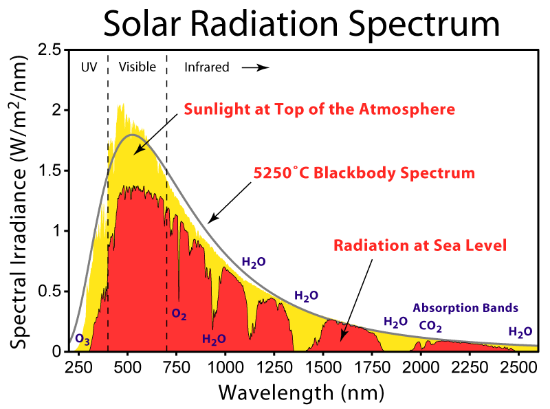
Gives you an idea how puny CO2 is in relation to all of the much broader and stronger bands controlled by water vapour.
water vapour is the control know , not CO2.
“When the orbit falls back to a lower orbit, it produces electricity.”
The photons knock the electrons free of atoms in the crystal lattice leaving behind a positive “hole”. The opposing charges are collected by fine wires and the voltage difference causes a current to flow in the external circuit.
Electrons can jump from one atom into a “hole” in a neighbouring atom and thus the holes can be regarded as being mobile. The charge mobility of both holes and electrons are one of the properties which are controlled and engineered in semiconductors .
Willis Eschenbach July 15, 2017 at 10:29 am
As anything with a temperature the atmosphere must radiate according that temperature. But imo a low density, low temperature gas can’t radiate enough energy to increase the temperature of the warmer oceans (or soil).
As you say, the photons just don’t have the energy required.
Pyrgeometers CALCULATE the amount of radiation they receive from the atmosphere.
http://www.kippzonen.com/Product/16/CGR3-Pyrgeometer#.WWsYq9Tyg1I
“The CGR3 is a pyrgeometer, designed for meteorological measurements of downward atmospheric long wave radiation. The CGR3 provides a voltage that is proportional to the net radiation in the far infrared (FIR). By calculation, downward atmospheric long wave radiation is derived. For this reason CGR3 mbodies a temperature sensor.”
For an actual MEASUREMENT I believe the instrument should be cooled to 0K and then measure how much the temperature rises when in radiative balance with the incoming radiation. I don’t see that temperature rise to ~278K when pointing the instrument upward to the night sky.
To explain our observed surface temperatures we don’t need any back radiation from the atmosphere.
see https://wattsupwiththat.com/2017/07/13/temperature-and-forcing/comment-page-1/#comment-2552384
For the oceans the mechanism is obviously different, but imo the TEMPERATURE of the deep oceans is completely set and maintained by geothermal energy.
Simply put, Earth has a temperature. The sun is not warming a blackbody from 0K to 255K or so.
It just increase the temperature of a shallow top layer which in turn warms the atmosphere.
Basic physics is that heat is radiated, conducted, convected. Welling is not a physics principal in the context of heat – up or down. ?dl=0
?dl=0
So, wot Greg said plus water heating is good because it integrates heat it acquires over an extended period in the high capacity energy store of the domestic water system/water heating system – depends if mains pressure or gravity header tank- for later use over a short period – on demand and when required, e.g. its not real time load balancing as pure electrical energy must always be, no batteries required, etc. NASA numbers on Slar Insolation Hope this helps
As I am here, you might like to consider this, a collection I just made. Ypu decide what is noise, and what happens next
https://www.dropbox.com/sh/7lfirzox1a0hpq4/AADLsIYVP5aa4iisnQOChI0Ca?dl=0
Try again, I don’t k like WordPress, or HTML. Gimme native Mac any day. ?dl=0
?dl=0
The most interesting part of this article is figure 8. In particular the lower part of the land data which shows an inverse relationship. This underlines why global average temps are not informative.
Hopefully he will be inspired to do a follow up looking at the geographical regions represented by the various bits of the land data scatter plot.
Most of that lower section must be Antarctica, with changes in TOA being driven by surface temps, not the other way around. The flat top to the red splash being tropics when temps are tightly regulated and insensitive to radiation changes.
Any where the surface of the earth is covered with water or ice, the surface temperature will be “tightly regulated” by the processes of evaporation/condensation and freezing/sublimation. The temperature will approach the measured dew point or frost point not the measured air temperature. Air temperature will never go below the dew point as long as there is moisture present.
The lower slope of the sea data at the top of figure 8 shows the feedbacks are at least 2 or 3 times stronger in the tropics and temperature is much tighter regulated there.
The lower red ( land ) data shows a totally difference regime working in Antarctica.
It would be worth properly identifying the regions contributing to the flat top in the red data too. Figure 8 is very informative. Good work by Willis.
On the large numbers of source enrgy and heat capacity I doubt the atmosphere is more than just a relatively low energy symptom/consequence of what the 1,000 times more heat energy containing oceans are doing, plus the imbalance of solar insolation the atmosphere may transfer. However this subject ignores one very powerful direct heating mechanism in the oceans, more powerful than radiatists can possibly imagine…
Whiie radiative energy through the criust is small, the effect of Petatonnes of magma continuously being reheated by our radioactive interior and recycled through the ocean floors evry 200 Million years, entering the oceans at 1,000 degree temperature delta is NOT. That’s real “Potential”, and serious heat capacity, transferred directly to the water, which is being continually warmed this way, more and less.
BTW there is some very made up physics above. Not even correct at High School level. Temperature exchange is driven by temperature gradient, not “potential”, which is used in other specialisations, gravity, chemical, electrical, but not thermal. There is no credibiity attached by those who make up their own beliefs, language and laws of physics to go with it, as they will not know what is proven science and what made up/hypothesis, and cannot communicate meaningfully with those who have studied the subject in oredr to understand it better, and discuss it with others sharing this knowledge. The whole point of a universal science language is precise exchange and learning. No point in commenting if you have not first mastered these basics. Science doesn’t care what you believe.
PS And magma flow through the thin basalt sea floor WILL vary asymetrically at a MIlankovitch maximum as the wafer thin 7km crust on our 12,000 Km th diameter hot rock pudding gets dragged about over the molten and semi molten mantle, bank=nging o into each other for the 1,000 years it takes to kick off an interglacial, creating new leaks along with the existing calderas and the molten core itself, 30% annual garvitational variation of a force 200 times te moon. There are roughly 1Million active volcanoes under the oceans, 100,000 over 1Km high. Mont Fuji wan’t born in a day, but it is only one ice age old, 100,000 years.
The gradient between 2(multiple) potentials.
Temperature is a measure of the collision of gaseous molecules . Kinetic energy being converted to heat energy. Think PV=nRT when thinking gradient.
You’re gong to have to stop explaining proven science established over centuries, people prefer to make up their own to fit whatver they believe at the time. The likes of Michael Mann and Paul Erlich for instance, the Josef Goebels of science approach, all with science denying agendas that put power and money above, honest, decent and truthful fact and the laws of physics.
PS It took a while before I realised, when doing water bottle rocket science, that PV has the units of energy. We were never taught that. I ended up with PV=mgh for the altitude reached w/o atmospheric drag and with instantaneous water discharge. People have done PhDs on this…. you can get a grant for anything, including science and plant denial as well data adjusting. as Michael Mann has again demonstrated.
PV is a result of gravity, the Pauli exclusion principle, and photons being the force carrier for changed matter.
Imagine if you could vaporize the water as it left the rocket how much higher it would go?
That’s the work you can do with water vapor.
Not if it vapourised outside the rocket, has to be action and reaction, so the phase change would need to drive the gas mass out of the bottle in the required direction. I do explain that the Saturn 5 and the Shuttle took off by blowing water vapour out their exhausts. Quite fast.
Yes I understand. Consider clear sky atm column, as rocket combustion chamber, with Sun pumping water vapor during day, settles and warms surface at night when late at night it starts condensing
If we could see it, it would look like this
https://micro6500blog.files.wordpress.com/2017/06/20170626_185905.mp4
micro6500 July 19, 2017, at 6:46 am
That might be so … but if so, please define precisely for us all the scalar field, the vector field, and the “unit of some quantity” that between the three describes potential radiation … no handwaving, please.
Thanks,
w.
Willis, I have got a request.
Figure 7. Long-term average surface temperature. CERES data, Mar 2000 – Feb 2016 is giving some interesting data:
Land: 8.7
Ocean: 17.5
Ant.: – 26.6
‘Ocean’ is supposed to be a better sun collector and a better ‘energy saver’ than ‘land’ is. The above numbers seem to confirm, but I don’t think the above numbers represent the right proportions. For example, because Antarctica (land) is that cold because of latitude, Antarctica will bring down the average number for surface temperatures of ‘land’ considerably. The same for ‘altitude’, as shown by Tibet in your figure: ‘high’ is represented by a low surface temperature because of the altitude. To be able to compare well, we need comparable numbers at ‘ocean level’ and from the same latitude.
Lacking skills myself to find this out, I want to ask you whether you can produce for every latitude (or every 10 degrees of latitude) the average surface temperature for land and for ocean grid cells. And the ‘land’ grid cells corrected for altitude. ‘Season’ (month) must have a large influence as well.
I think those data will give a good insight in the different latitudinal effects on the distribution of land temperatures resp. ocean surface temperatures. And so on the role ‘land’ and ‘oceans’ play at every latitude, at the NH and SH. The results could be very interesting.
Zonal differences are very important. For example the changes in ‘obliquity’ cause zonal changes, during seasons, but also on geological timescales. And those changes could be very equal in effect. Knowing this all will help us to understand better the climate mechanisms of the Earth.
Wim, thanks for the question. Do you mean something like this?
w.
Willis, thanks for the link, I’ve read your post ‘Temperature Field’. Interesting, nice maps, but not exactly what I wanted. I am very interested in absolute temperatures of ocean and land per latitude (!), corrected for elevation. I suppose (in combination with the maps) they will tell us more about the real role of the oceans.
As an example of what absolute temperatures can raise for questions (that can lead to interesting answers) I had a look at the numbers for surface temperatures in both posts. In your last post you included the data for two extra years: 2014 from March to 2016 to March.
First column: Data Mar 2000 – Feb 2014, fig. 1 of post‘Temperature Field’
Second column: Data (Mar 2000 – Feb 2016), fig. 7 of post ‘Temperature and Forcing’
Avg Globe: 15 (15.1)
NH: 15.7 (15.8)
SH: 14.4 (14.4)
Trop: 26.5 (26.6)
Arc: -11.9 (- 11.8)
Ant: – 39.6(– 26.6)
Land: 10.5 (8.7)
Ocean: 16.8 (17.5)
While the average temperature of the Earth as a whole remains nearly the same over the two periods, the last three items show unexpected temperature changes. The Antarctic temperatures over the whole period are that much higher than expected that I think there must be a typing error. The next two items, Land and Ocean are also remarkable. After two El Nino years average ocean temperatures rose quite a bit: 0.7 degrees. I think that is too much for average temperatures over the whole period. And land temperatures lowered (average over the whole period…..) with nearly two degrees (1.8). Given the difference in surface area of resp. ocean and land the numbers might be correct in comparison with the average globe numbers 15(15.1). But if they are correct, what is the explanation for the fact that warm El Nino years lead to lower land temperatures?
Here with the surface data of CERES more things might play a role. Technical things. Perhaps you can’t compare the two periods as I’ve done. But my point is that the absolute temperatures per latitude as requested (elevation corrected) might give some insight in the working of our present Interglacial – Pleistocene climate system. Maps will surely be interesting, but also a table with the absolute numbers, split for Land and Ocean per latitude. They will raise interesting questions, I suppose.
Ben Wouters July 23, 2017 at 7:57 am
True. I’d lose the all-caps, though.
Ben, I don’t understand this. As you point out, the geothermal flux is on the order of a tenth of a watt or so.
Given that … if there were no sun and no atmosphere, please provide an estimate of the surface temperature of the earth.
There’s a good explanation of pyrgeometers here … but I truly don’t understand your point here. Are you claiming that scientists around the planet are using pyrgeometers that are inherently faulty or inaccurate? Or that the scientists are not using them appropriately? I can assure you that they test these things …
Because if that is your claim … well … neither the scientists nor the manufacturers of these precision instruments are gonna pay any attention to you without hard verifiable evidence that that is the case. There’s a spec sheet for a couple commercial pyrgeometers here and here … let us know what problems you see with them.
Best regards, thanks for the comments,
w.
Willis Eschenbach July 23, 2017 at 7:54 pm
In that case the geothermal flux would be slightly higher (greater delta T over the crust) and the geothermal gradient consequently a bit steeper.
Surface temperature to radiate away this flux ~35-40K. (emissivity 1.0)
The deep mines I mentioned would now be very cold (< 100K) iso ~330K.
But when applying external warming to the surface, the flux is blocked, and the crust starts to warm, until the gradient is such that energy can be lost again at the surface.
On planet Earth the temperature just below the surface provides the base temperature on top of which the sun does its warming magic. Think solar Joules warming just ~50 cm of soil, or the upper 10 meter of water.
Sun delivers in one day normally 5 or 6 kWhr/m^2, just enough to warm 10 meter of water 0,5K or so.
http://www.pveducation.org/pvcdrom/average-solar-radiation
Looks like this:
For land see eg.
http://www.tankonyvtar.hu/hu/tartalom/tamop412A/2011_0059_SCORM_MFGFT5054-EN/content/2/2_1/image099.jpg
With the resulting surface temperatures, Earth loses on average ~240 W/m^2 to space since the atmosphere slows the energy loss compared to the ~390-400 W/m^2 the surface would radiate directly.to space without atmosphere.
Since the sun delivers ~240 W/m^2 on average, the energy budget is balanced at a much higher surface temperature than would be possible with a purely radiative balance as eg on our moon (average temperature ~197K)
Ben Wouters July 24, 2017 at 5:32 am
OK, in the absence of the sun we’d be at minus 235°C (-391°F). Seems about right.
Given that, I don’t understand your claim above that:
How does the fact that the earth would be extremely cold if the sun didn’t shine somehow mean that the sun is “able to warm the surface to our observed values”? I don’t see what one has to do with the other. Just because it would be cold without the sun doesn’t mean it would be 15°C with the sun, that makes no sense at all.
w.
Willis Eschenbach July 24, 2017 at 10:05 am
The geothermal gradient adjusts very slowly to the average surface temperature.
If eg the average surface temperature increases 10K, the flux can’t reach the surface anymore, and the entire crust begins to warm up until the gradient is re-established starting at the higher surface temperature and the flux can flow again, but It takes indeed a lot of time to warm up 25-70 km of rock 😉
see https://en.wikipedia.org/wiki/Geothermal_gradient#Variations
In the following gif a 24 hr display of 70 cm surface and 200 m air temperature reading on a calm, clear summer night nicely showing how a Nocturnal Inversion develops:
http://wtrs.synology.me/photo/share/Su74sMwt/photo_54455354_70726f6674616c6c202831292e676966
Notice how only the upper 20-30 cm of the soil reacts to solar warming and overnight cooling.
The “base temperature” at ~50 cm and below is caused by geothermal energy. (13 centigrade is roughly the yearly average temperature at that location)
I haven’t found any numbers yet for how long it takes for the geothermal gradient to re-establish to a 1K average surface temperature change. Very interested, especially the number for oceanic crust.
Ben, I’m sorry but I fear I have no idea what you mean in that explanation. It doesn’t make logical sense.
Look, the TOTAL possible contribution from geothermal heat is NOT regulated by the interior temperature. It is regulated by how fast it can make it through the surface. I’ve never seen any estimate of that contribution that is more than about a tenth of a watt/m2. And it would be about the same even if the earth were 50°C warmer or 50°C cooler.
The part it seems you are missing is that yes, 300 metres down in the earth it’s hot. And 300 metres down in the ocean it’s cold.
So what? That doesn’t make us any warmer or any colder.
We don’t live 300 metres down in the earth, and there is very, very little leakage of heat from the interior to the surface. We live at the surface, where we’re getting a trivial amount of heat from below.
w.
Willis Eschenbach July 24, 2017 at 4:47 pm
Wiliis, it seems we’re talking past each other.
To me temperatures at ~300 m in the oceans and ~15 m in the soil are a base temperature, not caused by solar energy. The surface temperatures are this base temperature plus what the sun adds to it.
see eg.http://www.oc.nps.edu/nom/day1/annual_cycle.gif
At ~150 m the temperature does not change throughout the year => no solar influence.
Surface temperature changes from ~4,5C to ~13C and back again in autumn and winter.
In the Cretaceous the deep ocean temperatures where ~20C or even higher, so the surface temperatures were correspondingly higher.
Do you agree with this?
In the energy budget for the continents the geothermal flux can obviously be neglected, relative to the solar flux. What imo can’t be neglected is the geothermally caused temperature just below the surface. Unless of course you claim that it doesn’t matter whether the temperature at 15 m is 0K, 100K, 200K or 290K, the surface temperatures will always be the same, caused by solar energy only..
Ben Wouters July 25, 2017 at 6:40 am
Thanks, Ben. Seems to me we’re in agreement. You’ve already said that without the sun, the surface temperature would be about 30°-40°K … which obviously has to be the “base temperature” above which there are further additions from the sun. Or as you said:
So yes, I agree with you. Base temperature is something like 30-40K “plus what the sun adds to it”.
Regards,
w.
Willis Eschenbach July 25, 2017 at 8:36 am
Don’t think you’ll find a temperature of 30-40K anywhere between the ~7000K inner core and the ~290K surface 😉 , but I’ll let the continents rest for now.
Good to see you agree with the base temperature of the oceans at around 4C,
This means that for ~70% of earth’s surface the temperature is already ~277K, before the sun starts to add anything. With an observed surface temperature of ~290K we only have to explain a ~13K difference for the surface layer to arrive at the observed surface temperatures.
Question is how much of this difference the sun delivers, and how much the atmosphere.
I go for 100% solar, but maybe a few percent can be attributed to the atmosphere.
This means that we do not need the 33K atmospheric warming the GHE claims to explain the surface temperature of the oceans and still have a balanced energy budget for planet earth:
We do however need to explain how the deep oceans got their temperature in the first place, and how eg they got so much warmer in the Cretaceous. I think I have a solid answer to those questions.
Ben Wouters July 26, 2017 at 12:57 am
Say what? That was YOUR ESTIMATE of the temperature of the surface without the sun, viz:
You go on to say:
Say what? That’s totally and completely untrue. I “agreed” to no such thing. QUOTE THE EXACT WORDS YOU ARE DISCUSSING, or this conversation is over. I will not stand for you putting words in my mouth like that.

We’ve already agreed, and you’ve already said, that the “base temperature” of the earth, which (I think) you are using to mean the temperature it would be without the sun, is on the order of -230°C. In other words, if the sun goes away, the oceans would freeze solid.
So where are you getting this nonsense about 4°C?
And why 4°C and not 0°C? Do you think that at the bottom of the ocean, the water is densest at 4°C?
Finally, it appears you are unclear about the two-way nature of the radiant energy flow between the atmosphere and the ground … while it is true that if I give you $100 and you give me $75 this can be represented by me giving you $25, that’s not what actually happened. In reality there were two flows of money, not one.
In the same way, in your graphic, you’re showing the radiation going one direction minus the radiation going the other direction. While again this can be correct as an overall change, it totally ignores the fact that in reality there are two flows of energy, not one.
Regards,
w.
Willis Eschenbach July 26, 2017 at 9:39 am
The 30-40K for earth is theoretical only, since earth has never been without sun.
It does happen on our moon, craters near the poles that never get any sunshine are at ~25K.
On the equator the sub-regolith temperature is ~220K, settled on the average surface temperature.
see http://earthguide.ucsd.edu/earthguide/diagrams/woce/
The dark blue 4C layer is roughly the depth where the sun has no more influence.
My point remains that the base temperature of the oceans is ~277K and of the continents around the average surface temperature for a specific location. These temperatures are completely caused by geothermal energy and the sun warms the surface layer on top of these temperatures.
The oceans have been created boiling hot, since they sat on more or less bare magma, and the temperatures of the DEEP oceans has been maintained by the geothermal flux plus occasional large magma eruptions like the 100 million km^3 Ontong Java one. For the continents the geothermal flux is sufficient to maintain the temperature of the entire crust as we see it today. (increasing 25K for every km you go down into the crust)
I do understand that the atmosphere radiates in all directions, since the direct radiation from the surface through the atmospheric window is a small part of the total radiation to space. I don’t see the atmosphere increasing the temperature of the surface, since imo solar energy is enough to explain the surface temperatures given the base temperatures as shown above. Possible exception (nocturnal) inversions, when part of the atmosphere is a bit warmer than the surface.
This is the “greenhouse effect” in operation at night, The surface cools, air temps drop, as temps near dew points more water vapor starts condensing. That radiates some 4J/g, some of which evaporates water that just condensed. This creates a lot of Dwlr and helps keep surface temps from dropping. It sacrifices evaporated water, and regulates to dew point temp. But only starts after rel humidity gets to higher levels, which in the temperate zones is usually late at night.
The effect of this on cooling is that it is nonlinear, cooling faster at dusk, and slower near dew point. This is in addition to the slowing from the 1/t^4 drop due to temp change.
Ben Wouters July 27, 2017 at 1:14 pm
I give up. I truly don’t understand you. You say that without the sun, the earth would be at – 230°C … but despite that you claim that the “base temperature of the oceans” is 277°K.
I have no idea what that means. It seems you are picking the temperature at the bottom of the ocean and calling that the “base temperature” and then adding in the sun.
But you’ve already agreed that without the sun the surface of the planet would be at – 230°C.
I’m sorry, but that makes absolutely no sense. You don’t get to just pick some number X band say that the temperature is that number plus solar input UNLESS that number X is the temperature minus solar input. That’s simple algebra. If:
Temperature = X + Solar Input
then
X = Temperature – Solar Input.
Since you’re not doing that, but you’ve already agreed that the number X (temperature without the solar input) is equal to -230°C, I don’t have a clue what you are talking about.
w.