By Sebastian Luening, Frank Bosse and Fritz Vahrenholt
Introduction
On 14th November 2016 Stefan Rahmstorf (“stefan”) of the Potsdam Institute for Climate Impact Research (PIK) published on the climate blog Realclimate an article entitled „Record heat despite a cold sun”. In this article he discusses a temperature prognosis which we first published 2012 in the book “Die kalte Sonne”. An English translation of the book came out 2013 under the title “The Neglected Sun”. In his blog post, Stefan Rahmstorf attempts to demonstrate that the solar development does not match with the temperature evolution and hence has only a negligible effect on climate. Furthermore, he argues that our temperature prognosis has essentially failed.
First of all, it is good to see that our work is being considered by a prominent climate scientist and by this has re-entered the public climate debate. Nevertheless, we disagree with the conclusions drawn by Stefan Rahmstorf and would like to take the opportunity to comment on the issues raised in his article. To this end, we address the following points:
· Is solar development really incompatible with temperature development?
· Does it make sense to evaluate a prognosis only a few years after it was published?
· How did we arrive at our prognosis and why do we think it will still be successful?
· How likely are high climate sensitivity scenarios?
1) Is solar development really incompatible with temperature development?
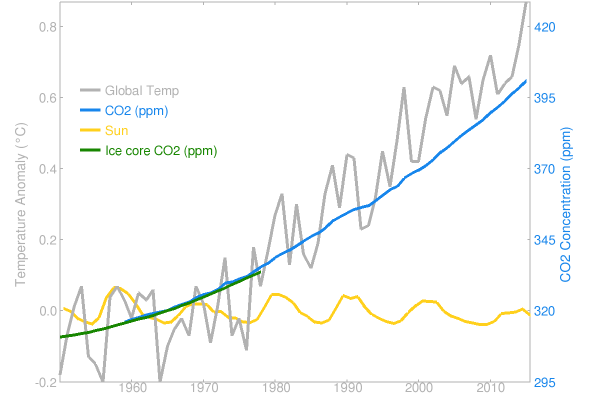
In his starting figure, Stefan Rahmstorf shows the time evolution of global temperature, CO2 concentration and solar activity from 1950 onwards. Unfortunately, the first part of the 20th century is not shown which would have offered interesting insights into possible climate driving mechanisms. In Figure 1 we have extended the graph to 1900 and illustrate solar activity based on a total solar irradiance (TSI) reconstruction by Steinhilber et al. (2009) based on cosmogenic radionuclide 10Be measured in ice cores. The rapid warming of the first half of the 20th century coincides well with a steady increase in solar activity. Attribution of this warming therefore is not trivial as also CO2 increased contemporaneously.
In the 1960s and 70s temperatures dropped, corresponding with a fall in solar activity while CO2 continued to climb upwards. Recent research suggests that the negative phase of 60 year ocean cycles may have been the main reason for this colder interval (Gervais, 2016; Meehl et al., 2016; Tung and Zhou, 2013). Solar activity picked up again in the 1980s/90s reaching some of the highest values, making the second half of the 20th century one of the most active solar periods of the past 10,000 years (Solanki et al., 2004).
Solar activity began to gradually decline in subsequent 11-year solar cycles in the 2000s and 2010s, as marked by the downward trend in the TSI curve by Steinhilber et al. (2009) (Fig. 1). Notably, the reduced solar activity roughly coincides with the so-called warming hiatus or slowdown that commenced around 1998. Again, ocean cycles may have played a major role in initially boosting and eventually terminating the phase of rapid warming that took place 1977-1998 (Meehl et al., 2016).
Due to the inertia of the climate system, time lags of a few decades with regards to external triggers have to be expected. The drop in solar activity during the early 21st century may therefore be only fully implemented in global temperatures in the coming years to decades, if solar activity plays a more important role than currently assumed by the IPCC. Stefan Rahmstorf’s solar representation misses the important ramp up to the exceptionally high solar plateau in the second half of the 20th century. Looking at the interval 1898 to 1997, solar activity (sensu Steinhilber et al. 2009) shows an even better (R=0.78) correlation with temperature than CO2 (R=0.75).

Figure 1: Time evolution of global temperature (GISS), CO2 concentration and solar activity (Steinhilber et al. 2009).
2) Does it make sense to evaluate a prognosis only a few years after it was published?
Climate change temperature prognoses refer to mid- and long-term developments, and do not intend to cover effects related to fast-paced El Nino, La Nina or volcanic events. It therefore does not make sense to evaluate a prognosis only four years after it was published, especially not during an El Nino year such as 2015/16. Apart from this, the temperature dataset chosen by Stefan Rahmstorf and its way of smoothing are debatable.
The GISS data have experienced repeated large administrative changes and therefore are considered by part of the climate research community as unstable (Fig. 2). Furthermore, Rahmstorf chooses averages over a 12 months period which unfortunately further emphasizes the El Nino peak. A better choice might have been monthly temperature data which by the time when Rahmstorf’s blog article went online in mid November 2014 had already returned down to values of the pre-El Nino temperature plateau. In terms of smoothing, a longer-term moving average would make better sense, e.g. 37 months, which helps to reduce some of the El Nino and La Nina short-term temperature effects. In the case of a 37 month smooth, the last smoothed data point is from mid 2015, shortening the reality-test interval of the prognosis down to merely three years.

Figure 2: Diagram showing the adjustments made since May 2008 by the NASA Goddard Institute for Space Studies (GISS) in anomaly values for the months January 1910 and January 2000. Graph from Climate4You.com (October 2016 newsletter).
In Figure 3 we have plotted the global RSS satellite temperature data for the period 1997-2016 and compared it with the prognosis of Vahrenholt & Lüning (2012). Since 2012 the 37-months RSS running mean has stayed quite well within the lower and upper limits of the prognosis. Short-term deviations outside the range during El Ninos and La Ninas are acceptable, as the dynamics of the temperature development have already exceeded the narrow range during previous occasions, e.g. during the 1998 El Nino (Fig. 3). The monthly RSS values in the second half of 2016 have sharply declined and have now re-entered the upper limit of the prognosis.

Fig. 3: Measurements of global temperature (RSS, monthly values, last data point October 2016) compared to the forecast for global temperature til 2030 by Vahrenholt & Lüning (2012: Figure 73). Thick line represents 37 months moving average.
The same comparison has also been carried out for the GISS surface temperature dataset (Fig. 4). In contrast to the satellite data, the GISS temperatures plot above the prognosed range. It will be interesting to see in the coming years, if the temperatures return into the corridor of the prognosis and if future administrative changes to the dataset by GISS will reduce the amount of perceived warming, possibly bringing better alignment with the satellite datasets.

Fig. 4: Measurements of global temperature (GISS, monthly values, last data point October 2016) compared to the forecast for global temperature til 2030 by Vahrenholt & Lüning (2012: Figure 73). Thick line represents 37 months moving average.
We take the opportunity to present additional temperature prognoses and their comparison with the measured temperature development. Meaningful comparisons can be carried out by studying climate scenarios that have been published at least two decades ago. First, we take a look at three temperature curves by Hansen et al. (1988) (Fig. 5). Scenarios B and C reflect cases in which trace gas growth rates would have been mildly reduced after 1988 and kept constant after 2000 (Scenario B), and drastically reduced 1990-2000 with zero emissions thereafter (Scenario C). The two cases have to be discarded, because emissions have not developed according to these scenarios, as we know today. Therefore scenario A captures the real evolution of emissions best, representing a 1.5% Increase of trace gas emissions per year, corresponding to growth rates typical of the 1970s and 80s. In terms of temperatures, however, scenario A of Hansen et al. (1988) has drastically overestimated warming by more than double the real amount.

Fig. 5. Measurements of global temperature (GISS, yearly average values) compared to the forecast for global temperature by Hansen et al. (1988). Description of scenarios see text.
Another temperature prognosis suitable for evaluation stems from the First Assessment Report (FAR) of the Intergovernmental Panel on Climate Change (IPCC) that was published in 1990. Since publication, 26 years of new data have been observed. The comparison shows that measured temperatures have followed a path at the lower end of the FAR climate scenarios (Fig. 6). Notably, the extreme upper warming forecast has turned out to be incorrect. A major factor in these scenarios plays the large range of 1.5-4.5°C of warming per CO2 doubling proposed by the IPCC FAR for the CO2 equilibrium climate sensitivity (ECS). The moderate warming that tracks the path at the lower end of the FAR spectrum may suggest that climate sensitivity is equally in the lower part of the IPCC range. Notably, an ECS scenario of 1.5°C was also presented by Vahrenholt & Lüning (2012).

Fig. 6. Measurements of global temperature (RSS, black curve) compared to the extreme lower (green curve) and upper (red curve) forecasts for global temperature by the IPCC First Assessment Report (1990).
3) How did we arrive at our prognosis and why are we confident that it will still be successful?
Our prognosis in Vahrenholt & Lüning (2012) considered three main climate drivers, namely an anthropogenic CO2 increase, multidecadal ocean cycles and solar activity changes.
CO2. In the years following our publication, a general shift towards lower CO2 climate sensitivities has occurred in the research community (Lewis and Curry, 2015; Loehle, 2014; Masters, 2014; Mauritsen and Stevens, 2015; Skeie et al., 2014; Spencer and Braswell, 2014; von der Heydt et al., 2014). The reduction is mostly based on re-evaluations related to the role of ocean cycles and the limited cooling potential of aerosols. Notably, reconsidered solar effects on climate have not yet been implemented and may lead to additional changes in the climate sensitivity value. In its latest report from 2013, the IPCC openly stated that at present it is not in a position to give a ‘best estimate’ for equilibrium climate sensitivity because of a “lack of agreement on values across assessed lines of evidence and studies”. To a certain extent, the re-considered warming potential of CO2 validates our prognosis approach in Vahrenholt & Lüning (2012) in which we used a climate sensitivity at the lower end of the current IPCC range of 1.5-4.5°C per CO2 doubling (IPCC, 2013).
Multidecadal Ocean Cycles. Since publication of our prognosis in 2012, the understanding of multidecadal ocean cycles and their systematic influence on global climatic has seen a major breakthrough. While previously modellers viewed the ocean cycles mostly as unpredictable noise, the cycles are now finally accepted to play a fundamental role in cooling or warming global climate. The Pacific Decadal Oscillation (PDO) and Atlantic Multidecadal Oscillation (AMO) have markedly increased global warming during 1860-1880, 1910-1940 and 1975-2000. In contrast, the ocean cycles slowed warming and cooled during 1880-1910, 1940-1975 and since 2000 (e.g. Han et al., 2016; Steinman et al., 2015; Tung and Zhou, 2013; Wyatt and Curry, 2014).
In the past, PDO peak plateaus typically triggered accelerated warming. Following the El Nino in 1998, the PDO has started its long-term decline, interrupted only by short-term rises, e.g. related to the recent 2015/16 El Nino (Fig. 7). The PDO climb down since 1998 may be the key reason for the slowdown in global warming since then. Based on an empirical average cycle period of 60 years, the PDO will most likely be in a general cooling stage during the coming two decades or so.

Fig. 7. Phases of the PDO ocean cycle Index compared to fluctuations in the general 20th/21st warming trend (monthly GISS data).
The AMO lags the PDO by about one and a half decades and started its decline only recently in 2015 (Fig. 8). The AMO cooling coupled with PDO cooling will turn the majority of the ocean cycle system into cold mode until the 2030s by when ocean cycles gradually turn into warm mode again.

Fig. 8. Atlantic Multidecadal Oscillation (AMO). From KNMI Climate Explorer. Last data point October 2016.
Solar Activity Changes. A great number of studies have demonstrated that solar activity has played a major role in climate during pre-industrial times (e.g. Hernández-Almeida et al., 2015; Holland et al., 2014; Ojala et al., 2015). On a Holocene scale of the past 10,000 years, solar-forced millennial-scale climate variability is a globally well-established Holocene phenomenon and has been described from all oceans and continents (Lüning and Vahrenholt, 2016). Solar-driven climate cycles are known from upper, middle and lower geographical latitudes, encompassing all climate zones, from the Arctic to the tropics. It is plausible to assume that the long-lasting connection between solar activity changes and climate is still active today.
Most solar physicists agree that we are heading towards a solar minimum in the first third or first half of this century (e.g. Ahluwalia, 2014; Lewis and Curry, 2015; Sánchez-Sesma, 2016; Skeie et al., 2014; Spencer and Braswell, 2014; Tlatov, 2015; Velasco Herrera et al., 2015; Zolotova and Ponyavin, 2014). In the past, solar minima have been commonly been associated with significant climate cooling, therefore it may be reasonable to expect a similar temperature effect in modern times for the coming decades.
How likely are high climate sensitivity scenarios?
In his blogpost at Realclimate, Stefan Rahmstorf cites a recent paper by Friedrich et al. (2016) in support of high climate sensitivities and a strong CO2 warming effect. The paper proposes massive anthropogenic warming of 5-7°C until the year 2100. This result is highly surprising because comparisons of modelled and measured temperatures favour rather lower climate sensitivity scenarios (see above). Also Brown et al. (2015) demonstrated that climate sensitivities in the upper part of the IPCC range are rather unlikely because they do not match with the observed recent temperature development, therefore worst case scenarios as envisaged e.g. by Friedrich et al. (2016) should be discarded.
In a recent post-publication review, James Annan demonstrated that the climate sensitivities proposed by Friedrich et al. (2016) grossly overestimate measured global warming (figure with Annan’s comparison here). Our own analysis confirms Annan’s results. We have digitized the key figure of Friedrich et al. (2016) and compared the output of the paper with the observations (Fig. 9). We used the ENSO-, solar- and volcano-adjusted global mean surface temperature (GMST) of Grant Foster (“Tamino”) since 1951 for four records (GISS, HadCRUT4, Cowtan/Way and Berkeley Earth). The comparison shows that the warming trend of Friedrich et al. is twice as high as the trend slopes of the observed GMST.
The calculated transient climate response (TCR) from the observations is 1.35°C per CO2-doubling, while the calculated TCR of Friedrich et al. amounts to 2.7°C per CO2-doubling. In a comment at James Annans Blog Nicholas Lewis determined an equilibrium climate sensitivity (ECS) of only 45% of the estimated values in the paper when using better established forcing data and GMST variances between Last Glacial Maximum and pre- industrial levels from recent studies in the literature.

Fig. 9. Model output temperatures from Friedrich et al. (2016) (red curve) compared to the observed adjusted measured temperature datasets of “Tamino”. Our prediction (Vahrenholt & Lüning 2012) is marked in brown. Note its small deviation to the observed temperatures in contrast to the large deviation of the red curve of Friedrich et al. (2016) which Rahmstorf cites as “sensitivity of global temperature to CO2 is independently confirmed by paleoclimatic data”
How did Friedrich et al. (2016) arrive at their conclusions which do not seem to hold up to reality calibration? The basis of their calculation is formed by temperature and CO2 data for the last nearly 800,000 years, covering several glacial and inter-glacial periods. Closer inspection shows that the authors seem to have overlooked that CO2 increases typically lag temperature rises by a few hundred years (Ahn et al., 2012; Monnin et al., 2001; Pedro et al., 2012; Stott et al., 2007) by way of CO2 outgassing from the warming oceans due to reduced ability to hold CO2 (Campos et al., 2016; Schmitt et al., 2012), making it complicated to attribute large parts of the warming to a primary carbon dioxide effect during Pleistocene times. Notably, the Friedrich et al. dataset has only a resolution of 1000 years which is insufficient to identify and discuss this time lag effect. In addition, James Annan discusses problems with the temperature database used by Friedrich et al. (2016). Summed up, the reasons for the exaggerated CO2 climate sensitivities of Friedrich et al (2016) may be found in incorrect attribution of warming, partial mix-up of cause and effect and choice of temperature reconstructions.
Conclusions
· Pre-industrial and 20th century data suggests that solar activity changes are a credible driver for climate change and require greater attention.
· While it is too early to judge our climate prognosis from 2012, it is essentially still well on track when eliminating short-term El Nino and La Nina effects.
· Comparisons of prognoses dating from 1988 and 1990 with subsequently observed data indicate that CO2 climate sensitivities are likely at the lower end of the spectrum proposed by the IPCC. Scenarios favoring high climate sensitivities significantly overshoot warming when compared to the real temperature development.
· Both Pacific and Atlantic ocean cycles have now entered into the multi-decadal cooling mode. Furthermore, also solar activity is expected to enter a major minimum phase. For the upcoming two decades it is therefore expected that natural climate drivers will contribute cooling to the climate system which may not be fully compensated by anthropogenic warming related to greenhouse gases.
· The climate system has arrived at an important crossroad at which it will soon become clear if the attribution of anthropogenic vs. natural drivers to 20th century warming has been quantitatively correct. It is expected that the coming 5-10 years will bring clarity to this question. We call on all parties of the climate discussion to open-mindedly engage in this critical phase, weighing the arguments and data for and against each other fairly and transparently, regardless of personal backgrounds, affiliations, previous convictions and individual preferences.
References
Ahluwalia, H. S., 2014, Sunspot activity and cosmic ray modulation at 1 a.u. for 1900–2013: Advances in Space Research, v. 54, no. 8, p. 1704-1716.
Ahn, J., Brook, E. J., Schmittner, A., and Kreutz, K., 2012, Abrupt change in atmospheric CO2 during the last ice age: Geophys. Res. Lett., v. 39, no. 18, p. L18711.
Brown, P. T., Li, W., Cordero, E. C., and Mauget, S. A., 2015, Comparing the model-simulated global warming signal to observations using empirical estimates of unforced noise: Scientific Reports, v. 5, p. 9957.
Campos, M. C., Chiessi, C. M., Voigt, I., Piola, A. R., Kuhnert, H., and Mulitza, S., 2016, Glacial δ13C decreases in the western South Atlantic forced by millennial changes in Southern Ocean ventilation: Clim. Past Discuss., v. 2016, p. 1-22.
Friedrich, T., Timmermann, A., Tigchelaar, M., Elison Timm, O., and Ganopolski, A., 2016, Nonlinear climate sensitivity and its implications for future greenhouse warming: Science Advances, v. 2, no. 11.
Gervais, F., 2016, Anthropogenic CO2 warming challenged by 60-year cycle: Earth-Science Reviews, v. 155, p. 129-135.
Han, Z., Luo, F., Li, S., Gao, Y., Furevik, T., and Svendsen, L., 2016, Simulation by CMIP5 models of the atlantic multidecadal oscillation and its climate impacts: Advances in Atmospheric Sciences, v. 33, no. 12, p. 1329-1342.
Hansen, J., Fung, I., Lacis, A., Rind, D., Lebedeff, S., Ruedy, R., Russell, G., and Stone, P., 1988, Global climate changes as forecast by Goddard Institute for Space Studies three-dimensional model: Journal of Geophysical Research: Atmospheres, v. 93, no. D8, p. 9341-9364.
Hernández-Almeida, I., Grosjean, M., Przybylak, R., and Tylmann, W., 2015, A chrysophyte-based quantitative reconstruction of winter severity from varved lake sediments in NE Poland during the past millennium and its relationship to natural climate variability: Quaternary Science Reviews, v. 122, p. 74-88.
Holland, H. A., Schöne, B. R., Lipowsky, C., and Esper, J., 2014, Decadal climate variability of the North Sea during the last millennium reconstructed from bivalve shells (Arctica islandica): The Holocene, v. 24, no. 7, p. 771-786.
IPCC, 1990, First Assessment Report http://www.ipcc.ch/publications_and_data/publications_and_data_reports.shtml.
-, 2013, Climate Change 2013: The Physical Science Basis. Contribution of Working Group I to the Fifth Assessment Report of the Intergovernmental Panel on Climate Change, Cambridge, United Kingdom and New York, NY, USA, Cambridge University Press, 1535 p.:
Lewis, N., and Curry, J. A., 2015, The implications for climate sensitivity of AR5 forcing and heat uptake estimates: Climate Dynamics, v. 45, no. 3-4, p. 1009-1023.
Loehle, C., 2014, A minimal model for estimating climate sensitivity: Ecological Modelling, v. 276, p. 80-84.
Lüning, S., and Vahrenholt, F., 2016, Chapter 16 – The Sun’s Role in Climate A2 – Easterbrook, Don J, Evidence-Based Climate Science (Second Edition), Elsevier, p. 283-305.
Masters, T., 2014, Observational estimate of climate sensitivity from changes in the rate of ocean heat uptake and comparison to CMIP5 models: Climate Dynamics, v. 42, no. 7-8, p. 2173-2181.
Mauritsen, T., and Stevens, B., 2015, Missing iris effect as a possible cause of muted hydrological change and high climate sensitivity in models: Nature Geosci, v. 8, no. 5, p. 346-351.
Meehl, G. A., Hu, A., Santer, B. D., and Xie, S.-P., 2016, Contribution of the Interdecadal Pacific Oscillation to twentieth-century global surface temperature trends: Nature Clim. Change, v. 6, no. 11, p. 1005-1008.
Monnin, E., Indermühle, A., Dällenbach, A., Flückiger, J., Stauffer, B., Stocker, T. F., Raynaud, D., and Barnola, J.-M., 2001, Atmospheric CO2 Concentrations over the Last Glacial Termination: Science, v. 291, p. 112-114.
Ojala, A. E. K., Launonen, I., Holmström, L., and Tiljander, M., 2015, Effects of solar forcing and North Atlantic oscillation on the climate of continental Scandinavia during the Holocene: Quaternary Science Reviews, v. 112, p. 153-171.
Pedro, J. B., Rasmussen, S. O., and van Ommen, T. D., 2012, Tightened constraints on the time-lag between Antarctic temperature and CO2 during the last deglaciation: Climate of the Past, v. 8, p. 1213-1221.
Sánchez-Sesma, J., 2016, Evidence of cosmic recurrent and lagged millennia-scale patterns and consequent forecasts: multi-scale responses of solar activity (SA) to planetary gravitational forcing (PGF): Earth Syst. Dynam., v. 7, no. 3, p. 583-595.
Schmitt, J., Schneider, R., Elsig, J., Leuenberger, D., Lourantou, A., Chappellaz, J., Köhler, P., Joos, F., Stocker, T. F., Leuenberger, M., and Fischer, H., 2012, Carbon Isotope Constraints on the Deglacial CO2 Rise from Ice Cores: Science, v. 336, no. 6082, p. 711-714.
Skeie, R. B., Berntsen, T., Aldrin, M., Holden, M., and Myhre, G., 2014, A lower and more constrained estimate of climate sensitivity using updated observations and detailed radiative forcing time series: Earth Syst. Dynam., v. 5, no. 1, p. 139-175.
Solanki, S. K., Usoskin, I. G., Kromer, B., Schüssler, M., and Beer, J., 2004, Unusual activity of the Sun during recent decades compared to the previous 11,000 years: Nature, v. 431, p. 1084-1087.
Spencer, R., and Braswell, W., 2014, The role of ENSO in global ocean temperature changes during 1955–2011 simulated with a 1D climate model: Asia-Pacific Journal of Atmospheric Sciences, v. 50, no. 2, p. 229-237.
Steinhilber, F., Beer, J., and Fröhlich, C., 2009, Total solar irradiance during the Holocene: Geophysical Research Letters, v. 36, no. L19704.
Steinman, B. A., Mann, M. E., and Miller, S. K., 2015, Atlantic and Pacific multidecadal oscillations and Northern Hemisphere temperatures: Science, v. 347, no. 6225, p. 988-991.
Stott, L., Timmermann, A., and Thunell, R., 2007, Southern Hemisphere and Deep-Sea Warming Led Deglacial Atmospheric CO2 Rise and Tropical Warming: Science, v. 318, no. 5849, p. 435-438.
Tlatov, A. G., 2015, The change of the solar cyclicity mode: Advances in Space Research, v. 55, no. 3, p. 851-856.
Tung, K.-K., and Zhou, J., 2013, Using data to attribute episodes of warming and cooling in instrumental records: Proceedings of the National Academy of Sciences, v. 110, no. 6, p. 2058-2063.
Vahrenholt, F., and Lüning, S., 2012, Die kalte Sonne, Hamburg, Hoffmann und Campe.
Velasco Herrera, V. M., Mendoza, B., and Velasco Herrera, G., 2015, Reconstruction and prediction of the total solar irradiance: From the Medieval Warm Period to the 21st century: New Astronomy, v. 34, p. 221-233.
von der Heydt, A. S., Köhler, P., van de Wal, R. S. W., and Dijkstra, H. A., 2014, On the state dependency of fast feedback processes in (paleo) climate sensitivity: Geophysical Research Letters, v. 41, no. 18, p. 6484-6492.
Wyatt, M. G., and Curry, J. A., 2014, Role for Eurasian Arctic shelf sea ice in a secularly varying hemispheric climate signal during the 20th century: Climate Dynamics, v. 42, no. 9, p. 2763-2782.
Zolotova, N. V., and Ponyavin, D. I., 2014, Is the new Grand minimum in progress?: Journal of Geophysical Research: Space Physics, v. 119, no. 5, p. 3281-3285.
Leif I will take a look at it.
Leif they did not convince me. They are making many unproven assumptions and it is their educated guess which is in line with your thinking.
Who knows for sure and at any rate TSI is not my main argument for solar /climate correlations.
https://arxiv.org/pdf/astro-ph/0201025v1.pdf
Another recent study.
Leif your position is to try to show that the sun is not variable and that it and associated secondary effects do not effect the climate.
My position is the opposite.
Time will tell.
On the TSI it is just hard to believe that the solar breakdown of it’s magnetic network was diminished as much during the very short solar lull of 2008-2010 versus the decades long length of the Maunder Minimum.
Leif your position is to try to show that the sun is not variable and that it and associated secondary effects do not effect the climate.
I don’t know really how to deal properly with such nonsense. There are several possibilities:
1) ignore it
2) engage in a protracted exchange of comments
3) cite some of my work that contradicts what you say
4) point out that science is not a set of ‘positions’ or opinions
5) take you out back and beat you up
Leif we disagree but every one disagrees not just us. The whole climatic issue is just one big disagreement and many tend to side with you and many tend to side with me.
Now I do appreciate your points of view but I have spent much time on this issue and came up with conclusions. I do not know if they are correct but this is what I have come up with.
I think Leif, what you have done for me is make me think more, make me question my conclusions more , and make me see things from another point of view.
Just because we do not agree does not mean I do not appreciate all of your efforts and your knowledge is extensive and you could be correct on every single point and maybe (I hope ) the clues may be forth coming the next few years.
I think to spend time with every one that has an opinion different then yourself is a very good service you provide to this website.
This website needs your points of view and I think you are going about it the correct way.
I do think highly of you believe it or not, and think you are good guy agree or not.
Good for you, Salvatore.
Thanks
Leif says
They differ between the 11-yr cycles. There are no Hale cycles in the energy.
henry says
I just looked at maximum temperatures where you live.
http://oi68.tinypic.com/fkqyi0.jpg
Tmax is a good proxy for energy coming through the atmosphere.
Funny: cannot find your 11 year Schwabe cycle there, but I do see my Hale \/ : exactly where I said it would be. We have to agree to disagree then. Again. So far I have:
1)Tmean before 50 years ago is not reliable.
2) SSN before 100 years ago is not reliable.
3) there is no Schwabe cycle. The Hale cycle is clearly visible in the Tmax record.
My prediction for the future:
One more Hale cycle of cooling coming up now. Sharp drop in T coming up very soon. We are now where we were in 1930. Only 2 years from the big dust bowl drought. 10 years away from the freezing 40’s.
That is going to cause some problems.
Yet, we have all these clowns here fiddling with their violins, completely clueless about climate change.
What a tragedy.
Hello!!! Do I need to remind everyone we are talking about the temperature of the earth, not the sun? This claim of tying the sun’s radiation to the earth’s temperature is the Climate Alarmists greatest non-sequitur. If I lay in a tanning booth, I will get a sun tan. If I lay in a tanning booth and put on SBF40 sunblock I won’t get a tan. What matters is the amount of solar radiation that actually reaches the earth, especially the oceans. Mother Nature isn’t stupid. I would imagine that if a hot sun can harm the earth, she has worked out a system to prevent it. My understanding is that a hot sun puts out greater intensity Cosmic Rays. Cosmic Rays seed clouds. Clouds block the sunlight from reaching the earth. What is important isn’t the sun’s radiation, it is the amount of radiation put out by the sun that actually reaches the earth to warm it. In addition to having ground temperature measurements, we should also have ground photometers measuring the energy actually reaching the earth? Does such a data set exist? If not, how can this be settled science? They are lacking data on the most important factor driving global temperatures.
Physicists claim further evidence of link between cosmic rays and cloud formation
A Danish group that has reproduced the Earth’s atmosphere in the laboratory has shown how clouds might be seeded by incoming cosmic rays. The team believes that the research provides evidence that fluctuations in the cosmic-ray flux caused by changes in solar activity could play a role in climate change. Other climate researchers, however, remain sceptical of the link between cosmic rays and climate.
http://physicsworld.com/cws/article/news/2013/sep/09/physicists-claim-further-evidence-of-link-between-cosmic-rays-and-cloud-formation
http://www.schillerinstitute.org/educ/sci_space/2015/0506-galactic_man_files/low_cloud_cover-vs-cosmic_rays-graph.jpg
lsvalgaard December 3, 2016 at 10:55 am
Leif, what’s the source of the 406-year data you show above?
w.
Figure 35 of
http://www.leif.org/research/Reconstruction-of-Group-Number-1610-2015.pdf
@Dan
We is us. The way we measure now.
all data sets of the past are corrupted to show AGW.
don’t trust the satellites too much either because there is no material that can withstand the sun for too long.
best is to make your own data sets.
it is not so difficult.
e.g. no data set shows we are cooling
yet we are: