Guest essay by Ferdinand Engelbeen
Both Bart Bartemis and Dr. Murray Salby are confident that temperature is the only/main cause of the CO2 increase in the atmosphere. I am pretty sure that human emissions are to blame. With this contribution I hope to give a definitive answer…
1. Introduction.
Some of you may remember the lively discussions of already 5 years ago about the reasons why I am pretty sure that the CO2 increase in the atmosphere over the past 57 years (direct atmospheric measurements) and 165 years (ice cores and proxies) is manmade. That did provoke hundreds of reactions from a lot of people pro and anti.
Since then I have made a comprehensive overview of all the points made in that series of discussions at:
http://www.ferdinand-engelbeen.be/klimaat/co2_origin.html
There still is one unresolved recurring discussion between mainly Bart/Bartemis and me about one – and only one – alternative natural explanation: if the natural carbon cycle is extremely huge and the sinks are extremely fast, it is -theoretically- possible that the natural cycle dwarfs the human input. That is only possible if the natural cycle increased a fourfold in the same time frame as human emissions (for which is not the slightest indication) and it violates about all known observations. Nevertheless, Bart’s (and Dr. Salby’s) reasoning is based on a remarkable correlation between temperature variability and the CO2 rate of change variability with similar slopes:

Capture: Fig.1: Bart’s combination of T and dCO2/dt from WoodForTrees.org
Source: http://i1136.photobucket.com/albums/n488/Bartemis/temp-CO2-long.jpg_zpsszsfkb5h.png
Bart (and Dr. Salby) thinks that the match between variability and slopes (thanks to an arbitrary factor and offset) proves beyond doubt that temperature causes both the variability and slope of the CO2 rate of change. The following will show that variability and slope have nothing in common and temperature is not the cause of the slope in the CO2 rate of change.
2. The theory.
2.1 Transient response of CO2 to a step change in temperature.
To make it clear we need to show what happens with CO2 if one varies temperature in different ways. CO2 fluxes react immediately on a temperature change, but the reaction on CO2 levels needs time, no matter if that is by rotting vegetation or the ocean surfaces. Moreover, increasing CO2 levels in the atmosphere reduce the CO2 pressure difference between ocean surface and the atmosphere, thereby reducing the average in/out flux, until a certain CO2 level in the atmosphere is reached where in and out fluxes again are equal.
In algebraic form:
dCO2/dt = k2*(k*(T-T0) – ΔpCO2)
Where T0 is the temperature at the start of the change and ΔpCO2 the change in CO2 partial pressure in the atmosphere since the start of the temperature change, where pCO2(atm) was in equilibrium with pCO2(aq) at T0. The transient response in rate of change is directly proportional to the CO2 pressure difference between the pCO2 change in water (caused by a change in temperature) and the CO2 pressure in the atmosphere.
When the new equilibrium is reached, dCO2/dt = 0 and:
k*(T-T0) = ΔpCO2
Where k = ~16 ppmv/°C which is the value that Henry’s law gives for the equilibrium between seawater and the atmosphere.
In the next plot we assume the response is from vegetation, mainly in the tropics, as that is a short living response as will be clear from measurements in the real world in chapter 3:

Caption: Fig. 2: Response of bio-CO2 on a step change of temperature
Source: http://www.ferdinand-engelbeen.be/klimaat/klim_img/trans_step.jpg
As one can see, a step response in temperature gives an initial peak in dCO2/dt rate of change which goes back to zero when CO2 is again in equilibrium with temperature. That equilibrium can be static (for an open bottle of Coke) or dynamic (for the oceans). In the latter case one speaks of a “steady state” equilibrium or a “dynamic equilibrium”: still huge exchanges are going on, but the net result is that no CO2 changes are measurable in the atmosphere, as the incoming CO2 fluxes equal the outgoing CO2 fluxes.
Taking into account Henry’s law for the solubility of CO2 in seawater, any in/decrease of 1°C has the same effect if you take a closed sample of seawater and let it equilibrate with the above air (static) or have the same in/decrease in (weighted) average global ocean temperature with global air at steady state (dynamic): about 16 ppmv/°C.
2.2 Transient response of CO2 to an increasing temperature trend.
If the temperature has a slope, CO2 will follow the slope with some delay.

Caption: Fig. 3: Response of bio-CO2 on a continuous increase of temperature
Source: http://www.ferdinand-engelbeen.be/klimaat/klim_img/trans_slope.jpg
A continuous increase of temperature will induce a continuous increase of CO2 with an increasing dCO2/dt until both increases parallel each other and dCO2/dt remains constant. This ends when the “fuel” (like vegetation debris) gets exhausted or the temperature slope ends. In fact, this type of reaction is more applicable to the oceans than on vegetation, but this all is more about the form of the reaction than what causes it…
A typical example is the warming from the depth of a glacial period to an interglacial: it takes about 5,000 years to reach the new maximum temperature and CO2 lags the temperature increase with some 800 +/- 600 years.
2.3 Transient response of CO2 to a sinusoid.
Many changes in nature are random up and down, besides step changes and slopes. Let’s first see what happens if the temperature changes with a nice sinus change (a sinusoid):

Caption: Fig. 4: Response of bio-CO2 on a continuous sinusoidal change in temperature
Source: http://www.ferdinand-engelbeen.be/klimaat/klim_img/trans_sin.jpg
It can be mathematically explained that the lag of the CO2 response is maximum pi/2 or 90° after a sinusoidal temperature change [1]. Another mathematical law is that by taking the derivatives, one shifts the sinusoid forms 90° back in time. The remarkable result in that case is that changes in T synchronize with changes in dCO2/dt, that will be clear if we plot T and dCO2/dt together in next item.
2.4 Transient response of CO2 to a double sinusoid.
To make the temperature changes and their result on CO2 changes a little more realistic, we show here the result of a double sinusoid for sinusoids with different periods. After all natural changes are not that smooth…:

Caption: Fig. 5: Response of bio-CO2 on a continuous double sinusoidal change in temperature
Source: http://www.ferdinand-engelbeen.be/klimaat/klim_img/trans_2sin.jpg
As one can see, the change in CO2 still follows the same form of the double sinusoid in temperature with a lag. Plotting temperature and dCO2/dt together shows a near 100% fit without lag, which implies that T changes directly cause immediate dCO2/dt changes, but that still says nothing about any influence on a trend. In fact still T changes lead CO2 changes and dT/dt changes lead dCO2/dt changes, but that will be clear in next plot…
2.4 Transient response of CO2 to a double sinusoid plus a slope.
Now we are getting even more realistic, not only we introduced a lot of variability, we also have added a slight linear increase in temperature. The influence of the latter is not on CO2 from the biosphere (that is an increasing sink with temperature over longer term), but from the oceans with its own amplitude:

Caption: Fig. 6: Response of Natural CO2 on a continuous double sinusoidal plus slope change in temperature
Source: http://www.ferdinand-engelbeen.be/klimaat/klim_img/trans_2sin_slope.jpg
As one can see, again CO2 follows temperature as well for the sinusoids as for the slope. So does dCO2/dt with a lag after dT/dt, but with a zero slope, as the derivative of a linear trend is a flat line with only some offset from zero.
This proves that the trend in T is not the cause of any trend in dCO2/dt, as the latter is a flat line without a slope. No arbitrary factor can match these two lines, except (near) zero for the temperature trend to match the dCO2/dt trend, but then you erase the amplitudes of the variability…
Thus while the variability in temperature matches the variability in CO2 rate of change, there is no influence at all from the slope in temperature on the slope in CO2 rate of change.
Conclusion: A linear increase in temperature doesn’t introduce a slope in the CO2 rate of change at any level.
2.4 Transient response of CO2 to a double sinusoid, a slope and emissions.
All previous plots were about the effect of temperature on the CO2 levels in the atmosphere. Volcanoes and human emissions are additions which are independent of temperature and introduce an extra amount of CO2 in the atmosphere above the temperature dictated dynamic equilibrium. That has its own decay rate. If that is slow enough, CO2 builds up above the equilibrium and if the increase is slightly quadratic, as the human emissions are, that introduces a linear slope in the derivatives.

Caption: Fig. 7: Response of CO2 on a continuous double sinusoidal + slope change in temperature + emissions
Source: http://www.ferdinand-engelbeen.be/klimaat/klim_img/trans_2sin_slope_em.jpg
Several important points to be noticed:
– The variability of CO2 in the atmosphere still lags the temperature changes, no matter if taken alone or together with the result of the emissions. No distortion of amplitudes or lag times. Only simple addition of independent results of temperature and emissions.
– The slope of the natural CO2 rate of change still is zero.
– The relative amplitude of the variability is a small factor compared to the huge effect of the emissions.
– The slope and variability of temperature and CO2 rate of change is a near perfect match, despite the fact that the slope is entirely from the slightly quadratic increase of the emissions and the effect of temperature on the slope of the CO2 rate of change is zero…
Conclusion: The “match” between the slopes in temperature and CO2 rate of change is entirely spurious.
3. The real world.
3.1 The variability.
Most of the variability in CO2 rate of change is a response of (tropical) vegetation on (ocean) temperatures, mainly the Amazon. That it is from vegetation is easily distinguished from the ocean influences, as a change in CO2 releases from the oceans gives a small increase in 13C/12C ratio (δ13C) in atmospheric CO2, while a similar change of CO2 release from vegetation gives a huge, opposite change in δ13C. Here for the period 1991-2012 (regular δ13C measurements at Mauna Loa and other stations started later than CO2 measurements):

Caption: Fig. 8: 12 month averaged derivatives from temperature and CO2/ δ13C measurements at Mauna Loa [9].
Source: http://www.ferdinand-engelbeen.be/klimaat/klim_img/temp_dco2_d13C_mlo.jpg
Almost all the year by year variability in CO2 rate of change is a response of (tropical) vegetation on the variability of temperature (and rain patterns). That levels off in 1-3 years either by lack of fuel (organic debris) or by an opposite temperature/moisture change [2]. Over periods longer than 3 years, it is proven from the oxygen balance that the overall biosphere is a net, increasing sink of CO2, the earth is greening [3], [4].
Not only is the net effect of the biological CO2 rate of change completely flat as result of a linear increasing temperature, it is even slightly negative in offset…
The oceans show a CO2 increase in ratio to the temperature increase: per Henry’s law about 16 ppmv/°C. That means that the ~0.6°C increase over the past 57 years is good for ~10 ppmv CO2 increase in the atmosphere that is a flat line with an offset of 0.18 ppmv/year or 0.015 ppmv/month in the above graph.
There is a non-linear component in the ocean surface equilibrium with the atmosphere for a temperature increase, but that gives not more than a 3% error on a change of 1°C at the end of the flat trend or a maximum “trend” of 0.00045 ppmv/month after 57 years. That is the only “slope” you get from the influence of temperature on CO2 levels. Almost all of the slope in CO2 rate of change is from the emissions…
3.2 The slopes.
Human emissions show a slightly quadratic increase over the past 115 years. In the early days more guessed than calculated, in recent decades more and more accurate, based on standardized inventories of fossil fuel sales and burning efficiency. Maybe more underestimated than overestimated, because of the human nature to avoid paying taxes, but rather accurate +/- 0.5 GtC/year or +/- 0.25 ppmv/year.
The increase in the atmosphere was measured in ice cores with an accuracy of 0.12 ppmv (1 sigma) and a resolution (smoothing) of less than a decade over the period 1850-1980 (Law Dome DE-08 cores). CO2 measurements in the atmosphere are better than 0.1 ppmv since 1958 and there is a ~20 year overlap (1960 – 1980) between the ice cores and the atmospheric measurements at Mauna Loa. That gives the following graph for the temperature – emissions – increase in the atmosphere:

Caption: Fig. 9: Temperature, CO2 emissions and increase in the atmosphere [9].
Source: http://www.ferdinand-engelbeen.be/klimaat/klim_img/temp_emiss_increase.jpg
While the variability in temperature is high, that is hardly visible in the CO2 variability around the trend, as the amplitudes are not more than 4-5 ppmv/°C (maximum +/- 1 ppmv) around the trend of more than 90 ppmv. To give a better impression, here a plot of the effect of temperature on the CO2 variability in the period 1990-2002, where two large temperature and CO2 changes can be noticed: the 1991/2 Pinatubo eruption and the 1998 super El Niño:

Caption: Fig. 10: Influence of temperature variability on CO2 variability around the CO2 trend [9].
It is easy to recognize the 90° lag after temperature changes, but the influence of temperature on the variability is small, here calculated with 4 ppmv/°C. For the trend, the CO2 increase caused by the 0.2°C ocean surface temperature increase in that period is around 3 ppmv of the 17 ppmv measured…
3.3 The response to temperature variability and human emissions:
With the theoretical transient response of CO2 to temperature in mind, we can calculate the response of vegetation and oceans to the increased temperature and its variability:

Caption: Fig. 11: Transient response of bio and ocean CO2 to temperature [9][11].
Source: http://www.ferdinand-engelbeen.be/klimaat/klim_img/rss_co2_nat.jpg
The bio-response to temperature changes is very fast and zeroes out after a few years [6], the response to the temperature amplitude is about 4-5 ppmv/°C, based on the response to the 1991 Pinatubo eruption and the 1998 El Niño.
The response of the ocean surface is slower, but stronger in effect. The 16 ppmv /°C is based on the long-term response in ice cores and Henry’s law for the solubility of CO2 in ocean waters (4-17 ppmv /°C in the literature).
In reality, both oceans and the biosphere are net sinks for CO2, due to the increased CO2 pressure in the atmosphere and the biosphere also a net sink due to increased temperature on periods of more than 3 years. That is not taken into account here, but is used in the calculation of the net increase of CO2 in the atmosphere with the introduction of human emissions.
If we introduce human emissions , that gives a quite different picture of the relative dimensions involved:

Caption: Fig. 12: Human emissions + calculated and measured CO2 increase + transient response of bio and ocean CO2 to temperature [9][11].
Source: http://www.ferdinand-engelbeen.be/klimaat/klim_img/rss_co2_emiss.jpg
The influence of temperature both in variability and increase rate is minimal, compared to the effect of human emissions, based on the transient response of oceans and biosphere and the calculated decay rate of human emissions.
The long tau (e-fold decay rate) of human emissions is based on the calculated sink rate (human emissions – increase in the atmosphere) and the increased CO2 pressure in the atmosphere above dynamic equilibrium (“steady state”), which is ~290 ppmv for the current weighted average ocean surface temperature. That is thus ~110 ppmv above steady state and that gives ~2.15 ppmv net sink rate per year. For a linear response, the e-fold decay rate can be calculated:
disturbance / response = decay rate
or for 2012:
110 ppmv / 2.15 ppmv/year = 51.2 years or 614 months.
That the sink process is quite linear can be seen in the similar calculation by Peter Dietze with the figures of 27 years ago [12]:
1988: 60 ppmv, 1.13 ppmv/year, 53 years
Or from earliest accurate CO2 measurements:
1959: 25 ppmv, 0.5 ppmv/year, 50 years
Conclusion: Within the accuracy of the CO2 emission inventories and the natural variability, the decay rate of any extra CO2 above the dynamic equilibrium (whatever the cause) behaves like a linear process…
3.4 The derivatives.
What does that show in the derivatives? First the transient response of the biosphere and oceans to temperature variability:

Caption: Fig. 13: RSS temperature compared to CO2 increase and transient response of natural CO2 (biosphere+oceans) rate of change [9][11].
Source: http://www.ferdinand-engelbeen.be/klimaat/klim_img/rss_co2_nat_deriv.jpg
It seems that the amplitude of the natural variability is overblown, but for the rest both the temperature and the transient response of CO2 are equally synchronized with the observed CO2 rate of change with hardly any slope in the transient response. Thus while all the variability is from the transient response, there is hardly any contribution of oceans or biosphere to the slope in CO2 rate of change.
The overdone amplitude of the natural variability may be a matter of CO2/temperature ratio or a too short transient response time, but that is not that important. The form and timing are the important parts.
Now we can add human emissions into the rate of change:

Fig. 14: RSS temperature compared to CO2 increase and transient response of natural CO2 + emissions rate of change [9][11].
Source: http://www.ferdinand-engelbeen.be/klimaat/klim_img/rss_co2_emiss_deriv.jpg
For an exact match of the slopes of RSS temperature and CO2 rate of change one need to multiply the temperature curve with a factor and add an offset. The match of the slopes of the observed CO2 rate of change and the calculated rate of change from the emissions plus the small slope of the natural transient response needed no offset at all: it was a perfect match. Only the amplitude of the variability was reduced, but that has no effect on the small natural CO2 rate of change slope.
As can be seen in that graph, both temperature rate of change and CO2 rate of change from humans + natural transient response show the same variability in timing and form. That is clear if we enlarge the graph for the period 1987-2002, encompassing the largest temperature changes of the whole period:

Fig. 15: RSS temperature compared to CO2 increase and transient response of natural CO2 + emissions rate of change in the period 1987-2002 [9][11].
Source: http://www.ferdinand-engelbeen.be/klimaat/klim_img/rss_co2_emiss_deriv_1987-2002.jpg
As is very clear in this graph, there is an exact match in timing and form between temperature and the transient response of the CO2 rate of change, as was the case in the theoretical calculations. Where there is a discrepancy between the observed and calculated rates of change of CO2 , temperature shows the same discrepancy, like the 1991 Pinatubo eruption which increased photosynthesis by scattering incoming sunlight.
Conclusion: it is entirely possible to match the slopes and variability by temperature only or by the effect of human emissions + natural variability.
4. Conclusion.
Which of the two possible solutions is right is quite easy to know, by looking which of the two matches the observations.
The straight forward result:
– The temperature-only match violates all known observations, not at least Henry’s law for the solubility of CO2 in seawater, the oxygen balance – the greening of the earth, the 13C/12C ratio, the 14C decline,… Together with the lack of a slope in the derivatives for a transient response from oceans and vegetation to a linear increase in temperature.
– The emissions + natural variability matches all observations. See: http://www.ferdinand-engelbeen.be/klimaat/co2_origin.html
Most of the variability in the rate of change of CO2 is caused by the influence of temperature on vegetation. While the influence on the rate of change seems huge, the net effect is not more than about +/- 1.5 ppmv around the trend and zeroes out after 1-3 years.
Most of the slope in the rate of change of CO2 is caused by human emissions. That is about 110 ppmv from the 120 ppmv over the full 165 years (about 70 from the 80 ppmv over the past 57 years). The remainder is from warming oceans which changes CO2 in the atmosphere with about 16 ppmv/°C, per Henry’s law, no matter if the exchanges are static or dynamic.
Yearly human emissions quadrupled from over 1 ppmv/year in 1958 to 4.5 ppmv/year in 2013. The same quadrupling happened in the increase rate of the atmospheric CO2 (at average around 50% of human emissions) and in the difference, the net sink rate.
There is not the slightest indication in any direct measurements or proxy that the natural carbon cycle or any part thereof increased to give a similar fourfold increase in exactly the same time span, which was capable to dwarf human emissions…
Conclusion: Most of the CO2 increase is caused by human emissions. Most of the variability is natural variability. The match between temperature and CO2 rate of change is entirely spurious.
5. References.
[1] Why the CO2 increase is man made (part 1)
[2] Engelbeen on why he thinks the CO2 increase is man made (part 2)
[3] Engelbeen on why he thinks the CO2 increase is man made (part 3)
[4] Engelbeen on why he thinks the CO2 increase is man made (part 4).
[5] http://bishophill.squarespace.com/blog/2013/10/21/diary-date-murry-salby.html?currentPage=2#comments
Fourth comment by Paul_K, and further on in that discussion, gives a nice overview of the effect of a transient response of CO2 to temperature. Ignore the warning about the “dangerous” website if you open the referenced image.
[6] Lecture of Pieter Tans at the festivities of 50 years of Mauna Loa measurements, from slide 11 on:
http://esrl.noaa.gov/gmd/co2conference/pdfs/tans.pdf
[7] http://www.sciencemag.org/content/287/5462/2467.short full text free after registration.
[8] http://www.bowdoin.edu/~mbattle/papers_posters_and_talks/BenderGBC2005.pdf
[9] temperature trend of HadCRUT4 and CO2 trend and derivatives from Wood for trees.
CO2 and δ13C trends from the carbon tracker of NOAA: http://www.esrl.noaa.gov/gmd/dv/iadv/
CO2 emissions until 2008 from: http://cdiac.ornl.gov/trends/emis/tre_glob.html
CO2 emissions from 2009 on from: http://www.eia.gov/cfapps/ipdbproject/IEDIndex3.cfm?tid=90&pid=44&aid=8
[10] The spreadsheet can be downloaded from: http://www.ferdinand-engelbeen.be/klimaat/CO2_lags.xlsx
[11] The spreadsheet can be downloaded from:
http://www.ferdinand-engelbeen.be/klimaat/RSS_Had_transient_response.xlsx
[12] http://www.john-daly.com/carbon.htm
Ferdinand Engelbeen,
I have agreed with you on this issue since I looked at it with some detail after watching one of Murray Salbys’ conferences. Furthermore this phenomenon was discovered in the early 70’s and correctly assigned to temperature induced vegetation changes by R.B. Bacastow, one of Keeling’s frequent collaborators.
I have two remaining questions if you would be so kind:
1) The changes in CO2 concentration due to vegetation seasonality appear to be at least twice as large as the amount that we put into the atmosphere every year and are very rapid as they take place in about 3 months. Does this contradict the belief by some climatologists that elevated CO2 levels will persist for thousands of years? It looks to me that if the biosphere can produce such rapid changes and increase its sink capacity it could very well take care of elevated CO2 levels in a few decades if no more CO2 is emitted. Am I wrong in your opinion?
2) The transient response of CO2 changes around the mean to temperature changes has been described as the carbon dioxide thermometer, as it provides an independent measure of temperature changes that agrees quite well with other measures (your figure 1). How good is that carbon dioxide thermometer in your opinion and is it capable of discriminating between satellite and land measurements as to which one constitutes a better fit to it? This has been argued, but not convincingly in my opinion.
Thank you.
Javier,
Thanks for the support…
About 1):
The fast growth and decay of leaves over the seasons, which absorbs a lot of CO2, but releases a lot of CO2 when the fallen leaves decay in the next year(s). That is about 60 GtC in and out each in a few months time over a year, but that doesn’t change much over the years.
The longer term uptake in more permanent storage (humus, peat, lignite, coal,…) is much smaller: currently about 1 GtC/year (~0.5 ppmv) for 110 ppmv increase in the atmosphere. That gives an e-fold time of ~220 years or a half life time of ~160 years. If I remember well, the IPCC gives an e-fold time of ~170 years for vegetation in its Bern model or a half life of ~125 years.
If the deep oceans were saturated (for which is no sign), vegetation should do all the work. That means that if we stop all emissions today, the decay to near equilibrium (5 half life times) would be over 600 years…
About 2):
Reverse engineering is a rather tricky business…
The high resolution ice cores show a drop of ~6 ppmv between MWP and LIA, corresponding to a global drop of ~0.4°C (at 16 ppmv/°C ocean surface equilibrium), half way Mann’s reconstruction (MBH’99) and others (Esper, Moberg,…). In current times, one sees a short time variability of 4-5 ppmv/°C (Pinatubo, El Niño), but in a rising CO2 rate of change, which makes it quite difficult…
I shouldn’t give it not too much weight…
So what you’re saying is that if mankind somehow created an increase in the acidity of the water cycle beyond the naturally buffered state that carbon dioxide exists in and started burning an ever increasing amount of flora and delayed flora which then released carbon dioxide into this no-longer buffered environmental cycle – it would explain the increases in environmental carbon dioxide suspended in the atmosphere.
Well then, its a good thing nobody on Earth causes acid rain anymore then, isn’t it?
It’s easy to show that Murray Salby is wrong in claiming that the CO2 increase is due to temperature rise. We use Henry’s Law, as Ferdinand points out:
This means that for every degree the globe warms, we expect the atmospheric CO2 levels to increase by about 16 ppmv.
We don’t have just theoretical calculations, however. We also have the Vostok ice core data for both temperature and CO2. This gives us a value of a change in CO2 due to temperature rise of ~ 16.5 ppmv/°C, in very good agreement with theory.
Now, since 1900 the CO2 levels went up by about 100 ppmv. For that CO2 increase to be due to warmer temperatures, it would require a temperature increase of 100 / 16 ≈ 6°C … and in fact the change in global temperature over that time was about 0.6°C.
In other words, the temperature change over the 20th century was a full order of magnitude too small to cause the corresponding increase in CO2.
Q. E. D.
w.
Willis,
Your above calculation is incorrect as you do not know the magnitude of the sinks and do not know what is the mixing of the deep ocean water with the surface ocean water. Also the entire ocean does not warm 1C, that is goofy. Your toy model calculation is silly.
William Astley November 25, 2015 at 12:29 pm
Thanks, William. Fortunately, we can estimate the magnitude of the sinks. We can calculate them on an annual basis. They are equal to the amount of CO2 emitted minus the change in CO2 in the air (both expressed in gigatonnes).
And while this assumes little change in natural sinks/sources, this assumption is strongly confirmed by the graphic above, which shows that observations and theoretical calculations agree very well, particularly post-1959 when we have good data on both emissions and CO2 levels. If there were significant natural variation in sinks and sources we’d see it in the graphic … but we don’t.
Also fortunately, the mixing of the deep and shallow oceans is what it is, but it doesn’t affect the above calculation.
I see I was not clear, my bad. I assumed that people would know that I meant the surface temperature of the ocean, which is the only temperature of interest in relation to the oceanic CO2 uptake/outgassing.
Subjective value judgements are not all that useful in a scientific discussion …
Best regards,
w.
Willis,
See my response and linked to paper below.
So, willis, your saying that bart’s graph is just a “coinkidink”? (maybe something is wrong with your analysis, not the data…)
The Vostok data are scarcely applicable to 20th century developments. The data are not proper (equi-spaced) time-series, with T and CO2 seldom shown concurrently. Under those circumstances the best that can be done is correlate total CHANGES in both variables over roughly matched time intervals. That R^2 is only ~0.1. This hardly provides any reasonable basis for causal attribution or for statistical reliance upon any regressional slope, especially when CO2 levels have risen well beyond those prevailing over most of the Vostok record.
The relationship is applicable surely, CO2 lags temperature.
sabretruthtiger:
The relationship in question is Willis’ claim of CONSTANT regressional dependence of 16ppmv CO2 per degree Celsius, which is scarcely validated by any phase-lagging of the CO2 signal in the Vostok data. On the contrary, any phase shifting invariably reduces the regressional slope, ultimately reaching zero for 90-degree phase shift. The 20th century CO2 levels, however, cannot be explained reasonably by any temperature-induced outgassing, as assumed by Salby.
1sky1 November 25, 2015 at 3:18 pm
Thanks, 1sky1, but that analysis is not all that is possible. A reasonable estimate of the relationship between the two can be done by interpolating the values of the more-sampled variable to match the less-sampled variable. Although this invariably reduces the peaks/valleys in the interpolated values, the amount is small for our purposes. I’m looking for an order-of-magnitude estimate, not three digit precision.
I don’t understand this claim. Why would the relationship between temperature and CO2 (confirmed by Henry’s Law) suddenly stop working just because CO2 levels have marginally increased?
1sky1 November 27, 2015 at 1:21 pm Edit
The calculation that I did was indeed the phase-lagged value, not the value at time zero. Since this is the real outcome, it reflects the something like the true strength of the actual change.
We are in total agreement about that. The effect of temperature on CO2 levels is an order of magnitude too small to explain recent changes in CO2 levels.
w.
Willis:
Henry’s law expresses the linear relationship between the partial pressure of a gas in the atmosphere and its equilibrium concentration in a liquid at FIXED temperature. This is a static law, not a dynamic prescription, such as required for establishing time-series relationships in non-equilibrium conditions. The very low correlation between roughly concurrent, quasi-millenial changes in T and in CO2 evident in the Vostok data, while partially the result of phase lag, shows us that such changes cannot provide a reliable empirical prescription through linear regression. The two variables simply are not very directly related. It is only at much longer time-scales, such as those of the Milankovitch cyles, that a very strong correlation, suggesting outgassing from oceans, can be found.
Hope this helps.
1sky1,
I plotted the Vostok data which gives:
http://www.ferdinand-engelbeen.be/klimaat/klim_img/Vostok_trends.gif
Which shows a rather linear ratio, which need to be doubled, as the temperature scale is at polar (snow) temperature changes.
I do find an R^2 of 0.75, not bad for a natural process, without taking into account the lags (~800 years with warming, several thousand years at cooling). Shifting the CO2 data back with lag times would make the correlation even better…
Further, the previous interglacial was ~2°C warmer than today: 290 ppmv CO2, according to the Vostok ice core…
Ferdinand:
Since CO2 and T are seldom given concurrently in the Vostok data, it is far from clear what was done to obtain your scattergram. It seems that you show the relationship between CO2 levels and long-term temperature anomalies for the fraction of data points that are nearly concurrent. This effectively compares well-correlated LEVELS at multi-millenial scales, over which equilibrium outgassing might have been achieved in conformance with Henry’s law, rather than comparing virtually uncorrelated, quasi-millennial CHANGES, which is the non-equilibrium issue at hand that I was referring to.
There’s a lot of discussion about Henry’s law above, but AFAICT there’s hardly anybody really challenging the formula for k for seawater, especially in the presence of a buffered system.
I can’t find a good graph for the ocean, but here’s a graph for human blood that suggests things aren’t so simple in the presence of soluble buffers:
http://2012books.lardbucket.org/books/principles-of-general-chemistry-v1.0/section_20/bf32c2157f7a9bce626717bd607a1244.jpg
from: http://2012books.lardbucket.org/books/principles-of-general-chemistry-v1.0/s20-06-buffers.html
I suspect the 16 ppmv/degC is something someone measured in a lab with seawater but no buffer – much like the many ocean pH experiments.
Does anyone have a definitive description of how that value was determined?
Peter
reading further, noted in a blockquote in the text:
The graph of blood plasma implies that the C02 is reacting with the solvent, and Henry’s law thus is not a simple constant. I suspect the same about the ocean.
Peter
http://2012books.lardbucket.org/books/principles-of-general-chemistry-v1.0/s17-solutions.html#averill_1.0-ch13_s04
Might have to buy this book if you really want to understand, it’s making my head explode already:
https://books.google.com/books?id=yRMgYc-8mTIC&pg=PA535&lpg=PA535&dq=henry%27s+law+in+a+buffered+system&source=bl&ots=OEJe7Bx2PB&sig=YAIdxH6Vg5VQgOnkayd41jVwuEA&hl=en&sa=X&ved=0ahUKEwihvsKXrK3JAhWCVYgKHU0oDZg4ChDoAQgcMAA#v=onepage&q=henry%27s%20law%20in%20a%20buffered%20system&f=false
I’d say one big assumption missing on that page already is the deep ocean mixing…. much of the ocean is actually shallow. (time to google that and find out the depth distribution vs. surface area of the ocean…)
Peter
Human blood has at least an order of magnitude more buffering agents than seawater has. For one thing, human blood in a healthy human body has around/over two orders of magnitude more organic compounds including amino, fatty and uric acids as well as biomass than seawater has, and at least an order of magnitude more bicarbonate and dissolved CO2.
Presumably you mean per unit volume. Are you sure? There’s an awful large amount of dissovable carbonate minerals on the ocean floor. Biomass, yes, I can see how the human has more biomass per unit volume of C02 than ocean. I was only referring to the available carbonates… both IMHO are equivalent to an open system, as much as you need, you can get. Generally when you have an open system on one side of a buffer and a closed system (C02 in the atmosphere) on the other side, thinks get… interesting. The metric that tends to vary is not the open system, it’s the closed system…
I was also just showing an example of blood plasma because I can’t find one for the ocean. All the textbooks I can find are “this is so”, not “here’s the data to prove it’s so”… silly textbook writers, they aren’t writing science, just factoids…
I’d like to see an equivalent curve for the ocean. Of course, since most of the pH experiments have been done incorrectly, good luck with that in a laboratory.
Yet again, another “we possibly don’t know”… though one could estimate from the Vostok cores, assuming there aren’t a pile of assumptions built into that one. Really need a prospective study…
Really I’m just challenging this hear to learn more about how Henry’s law deals with buffered systems where the availability of the dissovable buffer far exceeds the gas in question. I don’t think it’s as cut and dried as people think, but I’d love to see an experiment that proves it is.
Peter
Peter Sable,
Does anyone have a definitive description of how that value was determined?
With over three million measurements both in laboratories and underway ships via samples and automated equipment…
Seawater is a weak buffer itself, carbonate deposits don’t play a role at the surface, only on (very) long term with the deep oceans and coastal or in shallow seas.
The formula used to compensate for the temperature difference between the measurement device and the seawater at hull (in situ) temperature is:
(pCO2)sw @ur momisugly Tin situ = (pCO2)sw @ur momisugly Teq x EXP[0.0423 x (Tin-situ – Teq)]
More background at:
http://www.ldeo.columbia.edu/res/pi/CO2/carbondioxide/text/LMG06_8_data_report.doc
More brain breakers about the dissociation constants at:
http://www-naweb.iaea.org/napc/ih/documents/global_cycle/vol%20I/cht_i_09.pdf
Contains at page 7 tables for the different dissociation constants for different temperatures and salinity and graphs at the next page…
At page 20, Fig. 9.10 gives the solubility of CO2 at different temperatures
At last the Bjerrum plot gives the relative abundance of the three C species at different pH’s:
https://en.wikipedia.org/wiki/Bjerrum_plot
Ferdinand, thanks for the links to the Bjerrum plot.
The very first sentence in the wikipedia is part of the same problem I and others are having with laboratory experiments concerning decreasing ocean pH.
The solution called the ocean isn’t at equilibrium – it’s not a closed system on the bottom end. About 15% of the earth’s surface is shallow ocean water with plenty of carbonate deposits and life to spread or absorb more carbonates to/from the other 55% of the earth’s surface and plenty of mixing to have this happen in a short time period. This is not being replicated in the lab.
I’d like to see a plot where the assumption of non-equilibrium (an open system on both the atmosphere and the ocean bottom/sealife) is characterized.
Peter
Figure 9.10 seems to be more what I was referring to: An open system on both ends, though I think one of the problems is really the atmospheric concentration is NOT an open system, as the amount of carbonates far exceeds the amount of C02 in the air (by mass).
http://www-naweb.iaea.org/napc/ih/documents/global_cycle/vol%20I/cht_i_09.pdf
The problem is in order to make this 4 variable 4 equation system easier to solve, they chose the wrong variable to fix:
This makes interpretation hard, but I’ll try.
If you peer closely at the log plot (log on X axis), at a pH of 8, the partial pressure of C02 changes slightly with temperature, with a resulting increase in the concentration of metals. The change, however (given 4 points close on a graph) is not linear. I’ll note this is a log scale, which means there’s a dramatic change in soluability with temperature if we’re talking ppm on a linear scale, which is how most of us refer to C02 concentrations. This will also increase any nonlinearities as can be (barely) seen by those 4 points plotted at pH of 8.
I’ll note that this plot (figure 9.10) is NOT replicated in the lab, and especially not in ocean buckets off of ships, because those are closed systems on one end – there’s no carbonate deposits on the bottom of the bucket (unless they let the barnacles grow…). So those 3M measurements are just repeating the possibly bad assumption of the linearity of Henry’s Law.
So figure 9.10 helps confirm my suspicion that the assumption of closed systems in Henry’s law is suspect. However, I’m still learning here, so please point out where I’m wrong. I think what I need is another several dozen data points around a pH of 8 for this plot. I’ll dig through the equations and see if I can do it myself. Time to find that open source algrebra solver, I’m not doing this by hand…
Peter
As for this:
http://www.ldeo.columbia.edu/res/pi/CO2/carbondioxide/text/LMG06_8_data_report.doc
Interesting reading especially with my background in metrology, but doesn’t address Henry’s law issues:
(1) they didn’t measure pH, and that’s pretty important. AFAICT they didn’t measure ion concentrations either.
(2) they did measure different levels of pC02 in the air and water and one at first glance might think that’s enough to draw a curve, but there can also be different unrelated changes in pH and ion concentration, the ocean isn’t instantaneously that well mixed and their measurements are from a whole ocean standpoint instantaneous measurements in time and space. We here are trying to use Henry’s law to estimate the entire ocean’s behavior over decades. Completely different scale.
So again I remain somewhat skeptical that Henry’s law is linear with respect to temperature and pC02 for the entire ocean on decadal time scales, because Henry’s law as commonly used makes lots of assumptions about how closed the system is. In fact the system is somewhat closed on the wrong end of the assumptions (the atmopshere) and open on the other end (the shallow ocean floor).
Eagerly look forward to someone proving me wrong here, because I’ll learn something.
Peter
Willis, the sink is not the same over time. In 1965, the sink was 6 bmt, today that sink is 19 bmt (NOAA). If it wasn’t that large, there would be some serious problems with co2 levels. The ppm would be 5.5 ppm not 2.5. As it is the total should be about 7 total divided by the sink and making its way into the atmosphere. In other words, the sink is larger than the amount making its way into the atmosphere.
Out of the 38 bmt, 4.5 ppm was absorbed, and 2.5 ppm in the atmosphere… more or less.. on the high side 8, low side would be 6.
I’ve seen using a different method that also had the temperature an order too large.
I provide a more accurate toy model somewhere below which refutes this argument. I am currently working my way down there to see what silly objections have been raised in my absence.
This is circular reasoning, Willis. You assume a model. You parameterize the model based on observations. And, then you conclude that the model matches observations.
Nobody appears to have thought the obvious. All the Ice Core studies I have read show that CO2 increases 800 years (+/- a few) AFTER temperature rises. Go back 800 years and what do you find but the Medieval Warm Period. Could this be the real reason for the increase in CO2?
Please see my comment http://wattsupwiththat.com/2015/11/25/about-spurious-correlations-and-causation-of-the-co2-increase-2/comment-page-1/#comment-2079960
Spurious correlations are extremely common in all areas of research. I never did stop eating butter or bacon, but that research was beyond spurious and simply false information like most of agw supporting studies.
Best article ever, the technical content of the article and the ensuing comments makes my head hurt trying to learn and figure both (Many) side of the argument, rather than the normal rumbling comments, I even need a pencil and paper.
The main effect of this good read was eluding the bliss of domestic evening chores.
long may we argue
First of all thanks for such a thorough article.
There’s still a lot I don’t understand but one detail stands out: why would the net sink increase in the same proportion as man-made emissions?
You’ve made this point a few times in the comments: emissions have more or less quadrupled since 1950s. But why, if the yearly natural sink is 100ppmv and the net was only 0.5 back then, would the net grow four-fold to just over 2ppm now? I assume that with global greening natural sink (and therefore net) would grow, but a net growing to 2ppmv would imply that natural sink grew from 100 to 101.5ppm or so (I know, I know, rough numbers).
Now, there’s nothing strange about natural sinks growing a little bit, but growing enough to offset half of man-made emissions, over this 60-year period, seems weird. Isn’t that a massive coincidence? Some process nobody has figured out yet? Or perhaps the numbers just aren’t so accurate and I’m reading too much into this ‘proportion’?
I just wanted to make clear that where I say ‘natural sink was is 100ppm’, or whatever other value, it’s just for reference. I know that the exact value isn’t known with such detail. The thing is that variations in this natural sink rate seem to have offset about half of man-made emissions, and I have no idea why that could be.
OTOH, if this net natural sink continued, stabilizing ppm would require FAR less drastic emission reductions than the UN and carbon budgeters have argued for. Meaning, if net sink is just over 2ppm, then cutting emissions in half (from 4.5ppm to 2.25ppm) would effectively leave us with stable concentrations. Crisis averted!
Of course cutting emissions in half is probably impossible in the next decades, but it’s far, far easier than cutting them by 80% or whatever other number the loons come up with. Now I see why this wouldn’t fit the ‘alarmist’ narrative – we can simply implement emissions cuts at a later date, if CO2 happens to be that dangerous.
Alberto Zaragoza Comendador,
In fact, the near linear increase in sink rate is the result of a slightly quadratic increase of human emissions over time. That leads to a slightly quadratic increase in the atmosphere and that gives a slightly quadratic net sink rate.
Any quadratic increase gives a linear slope in the derivatives. Thus a quadrupling in the yearly emissions or the past 57 years gives a quadrupling of yearly increase in the atmosphere and a quadrupling of the net sink rate per year.
That is a question of pressure difference between CO2 in the atmosphere and in the oceans (vegetation helps too, but oceans are the main sinks). If the atmospheric pressure increases, the release of CO2 at the equatorial upwelling is decreased and at the polar sink places the sink rate is increased. The net sink rate is in rather linear ratio to the pressure difference between atmosphere and oceans; if that doubles, the sink rate doubles…
And you are right: if we could reduce human emissions to equal the sink rate, CO2 levels would stay at the current level. If necessary at all…
Net sink is proportion to how away-from-equilibrium the atmosphere is with the sum of the hydrosphere and biosphere.
Sorry Ferdinand, you are drawing incorrect generalised conclusions by looking at very special cases: pure sinusoids and constant linear increase.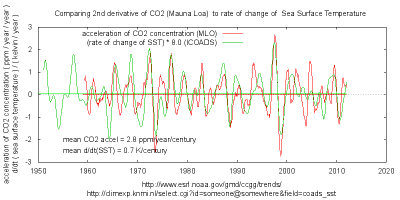
The linear relaxation response that you are using has a frequency dependent amplitude. It will be less for inter-decadal variation that it is for inter-annual variation.
Values for this at two time-scales are estimated from HadSST3 and Mauna Loa CO2 here:
https://climategrog.wordpress.com/?attachment_id=233
Centennial scale will be smaller again, I’d guess about 2 ppm/year/kelvin from those values.
If we takes 0.7K/century rise as the centennial scale temperature variation that gives about 140 ppmv increase due to out-gassing which is about the rise since pre-industrial levels.
Now that 2 ppm/year/kelvin was a pretty crude estimation so maybe we should say 2+/-1 ppm/year/kelvin. It still mean a significant part of CO2 rise could be outgassing.
Mike,
Sorry, but you make the same mistake as Bart: the response of oceans and vegetation to a temperature change is in ppmv/K not ppmv/K/period. A fixed temperature change of the ocean surface gives a fixed CO2 change in the atmosphere, per Henry’s law, no matter if that is static (of a closed sample) or dynamic (all over the ocean ins and outs). It is a transient response at ~16 ppmv/K, not a continuous fixed or accelerating increase in the atmosphere for a fixed temperature step.
I have focused on the simple sinusoids (+ “emissions”), because the theory proves that a linear increase in temperature gives hardly any slope in the derivatives of the transient response of CO2 in oceans and vegetation. If one then applies the same rules to the real temperature data, a slight slope is visible, just enough to match the observed slope of total CO2 rate of change together with the calculated increase rate due to human emissions.
Your 2 ppm/year/kelvin includes both the small rise by the transient response and the rise due to human emissions. In that way, you attribute human emissions to the temperature rise…
What I did show is that the variability is entirely natural and mostly temperature variability induced. The slope of the rise may be temperature induced or human induced, but the latter fits all observations, the former none, except a similar fit of the variability and the slope of the graphs…
So many words, graphs, “conclusions” (convincing only those who make them)…
All this in the face of one undeniable fact: in reality, there was no statistically significant increase in temperature since 1940 if we remove all the falsification (“adjustments”) from the temperature data. Your arguments, gentlemen, are about a wisp of imagination, and play into the hands of the data torturers and ignorant, corrupt politicians.
The following satellite data contained in the document below displays a “pause” in CO2 starting around 2005. Please look at the graph of the ACOS data As supports Dr. David Evans “Notch Theory” research which predicted a decrease in temprature starting around 2005.
http://disc.sci.gsfc.nasa.gov/featured-items/airs_acos_co2_satellite_observations
Figure 6. Time-series of globally averaged CO2 mixing ratios from AIRS Version 5 (2002-2012) and ACOS Version 2.9 (2009-2012). A subset of the ground observations record at Mauna Loa Observatory (1982-2012) (Tans and Keeling, 2012) is given for reference.
Figure 2. The mid-infrared spectrum of clean air in a 24 m cell. Main absorption bands of target gases CO2, carbon monoxide (CO), and water vapor (H2O) are shown. [After Howard (1959) and Goody and Robinson (1951)].
Oddly or paradoxically the reason why there was a 80 ppm to 100 pm drop in atmospheric CO2 during the recent glacial/interglacial cycles is not known. The calculation of CO2 pluses and minuses during the glacial cycle can only account for a lower of 8.5 ppm.
This fact indicates that there are multiple incorrect assumptions concerning the sinks and sources of CO2.
A back of the envelop calculation of the CO2 variance divided by the temperature change for the glacial/interglacial cycle has therefore zero relevance concerning Salby’s assertions.
http://courses.washington.edu/pcc588/readings/Sigman_Boyle-Glacial_CO2_Review-Na00.pdf
“A back of the envelop calculation of the CO2 variance divided by the temperature change for the glacial/interglacial cycle has therefore zero relevance concerning Salby’s assertions.”
Any comparison of what happens during a switch from one quasi-stable climate state to another has no relevance to short term change during stable conditions of an interglacial.
With massive changes to both the biosphere and crypsphere it is foolish to try to infer anything about present variation and causation by looking at de-glaciation transitions.
The ice age glaciations had so much temperature drop that according to the Henry’s Law rules, atmospheric CO2 concentration would have dropped a lot. And glaciations that caused dying-off of vegetation would have trapped some of that dead vegetation under ice/snow, so that would have become CO2 the next time the situation thawed out. From over 400,000 years ago to less than 150 years ago, CO2 did lag temperature by (on average and not constantly) 800 years, while the sum of carbon in the atmosphere, hydrosphere and biosphere was largely constant, and CO2’s role as a greenhouse gas was to contribute to positive feedback of climate changes initiated by other causes. Warmer temperatures caused CO2 to shift to the atmosphere to cause positive feedback for warming, and likewise the inverse for cooling. Within the past 150 years, there has been a new activity of transferring carbon from the lithosphere to the sum of the atmosphere, hydrosphere and biosphere – human combustion of fossil fuels.
William Astley,
“the reason why there was a 80 ppm to 100 pm drop in atmospheric CO2 during the recent glacial/interglacial cycles is not known”
It is not know for certain, but from the papers I’ve read the general opinion among scientists working in the field is that it is due to changes in ocean circulation. There is a constant flux of carbon from the surface ocean to the deep ocean in the form of dead organisms. They decompose in the deep ocean and the CO2 is returned to the surface and atmosphere by upwelling. A reduction in upwelling means less return of CO2, resulting in a drop of atmospheric CO2. There seems to be little, if any, agreement on the cause of changes in ocean circulation.
All these comments prove one thing very clearly….THE SCIENCE IS NOT SETTLED !!!
What is the exact definition of your statement “THE SCIENCE IS NOT SETTLED !!!”?
Nick Stokes:
Hey, if you integrate everything into straight lines; add arbitrary scaling and an offset you can make anything match. That last graph means nothing.
Having filtered out the annual seasonal cycle, it is quite clear from the differential what the relationship is between T and CO2 on an decadal scale. Sadly we don’t have reliable CO2 data back before Keeling started his work, so it’s not possible to accurately scale the relationship on longer time scales but we can estimate it.
Temperature since 1957 is not a straight line so Ferdinand’s attempt to draw conclusions by pretending it is is invalid.
Here is another graph estimating the inter-decadal scaling at about 3 ppm/year/kelvin and clearly showing it to be much stronger on inter-annual scales.
https://climategrog.wordpress.com/?attachment_id=223
Neither temp nor CO2 can be reasonably called a straight line.
In this graph we see, apart from the scaled CO2 / T relationship, a rise of 1 ppm/year around 1960 and twice that now. This could be a response to long term warming, residual anthropogenic emissions or a mixture of both.
I don’t think that there is enough data to extact any more information than that.
Mike,
Where did I use straight lines besides Fig. 3?
I did use several different theoretical variants, including a double sinusoid with and without a slope.
The latter shows that “temperature” and dCO2/dt from a transient response show an exact match in timing and form of the variability. So do the real values. But temperature has a slope and dCO2/dt has no slope in the theory and only a very slight slope in real data.
That means that most of the slope in the real life CO2 rate of change is not caused by temperature but by human emissions…
Here’s another view of the data:
https://climategrog.wordpress.com/?attachment_id=223
Sorry Ferdi, No straight lines anywhere.
Looking forward to Dr. Salby’s reply…
TomRude,
Already waiting over a year to have any of my objections answered…
The increase in CO2 is mostly due to man made emissions. Of course, we are talking about CO2 levels below 1000 PPM and very unlikely to ever exceed that. Such levels are low versus geological history.
The last 500 million years of substantial atmospheric CO2 with no sustained temperature change is compelling evidence CO2 has no effect on climate. This is documented in a peer reviewed paper at Energy & Environment, Volume 26, No. 5, 2015, 841-845 and also in http://agwunveiled.blogspot.com which also discloses the two factors that do cause reported average global temperature change (sunspot number is the only independent variable). The match between calculated and measured is 97% since before 1900.
This is exactly what every popular Internet forum degenerates into as it ages: a posturing ground of a few shrill peacocks proving to each other their obsolete points of view and dressing down anybody who reminds them of reality.
Reality being that nothing, absolutely nothing happened with the climate or with the Earth’s temperature during the last few decades of observation that is not deep within the range of natural variation.
For every single reasonable human being on this planet there are hundreds of Ferdinands and Willises, for whom their little smarting egos are more important than truth, dignity, and anything else. Disgusting.
Amen, alexander, (unfortunately) well said…
Alexander Feht:
For every single reasonable human being on this planet
Where Alexander Feht is the last man standing?
I didn’t say one word about the influence of CO2 on climate and used the satellite temps as most reliable (if not, write your complaints to the RSS people).
Any real scientific objection against what I wrote about the cause of the CO2 increase?
If there is no influence of CO2 on climate, then the whole conversation about it is moot. If there is, your not saying a word about it makes the whole conversation moot.
The discussion/debate on this thread is very interesting. I am exhausted just following it all and will likely return for an encore reading again when time allows.
I hope that this discussion/debate will be recognized by some true unbiased academic professors and will be required reading for their students.
This is WUWT University in action. No other place offers such an exchange of ideas from the level of participants as is being offered here and now! This is absolute brain candy! Please continue.
Thanks to all commenters. And as noted in an earlier comment by Richard Courtney …”Those are three different explanations of alternative possibilities to the narrative you promote and there is not sufficient data to resolve which – if any – of them is correct. …. ”
It’s not quite as simple as we were told by the so-called “climate science” establishment 10 years ago.
The use of Henry’s law in this context is not valid because Henry’s law only refers to the equilibrium between atmospheric CO2 and CO2 dissolved in seawater. However most (ie: about 97%) of the CO2 in seawater is in the form of carbonate and bicarbonate ion. These ions have no impact on Henry’s law at all yet CO2 can migrate rapidly and readily between CO2, HCO3- and CO3= . If the ocean warms and some of the dissolved CO2 goes back into the atmosphere that will increase the pH of the ocean – make it more basic (reduce the carbonic acid level) and the feedback response will be for more carbonate to move to bicarbonate and more bicarbonate to move to dissolved CO2. Thus the 16 ppmv/C is not correct, the sensitivity is actually much higher.
interesting hypothesis. data?
The ocean-atmosphere chemistry is reasonably stable. Climate sensitivity to manmade increase of CO2 is looking low enough for increase of atmospheric CO2 to increase ocean concentration of bicarbonate and H+ ions (slightly reduced pH, slightly more acid). The pH change to less-alkaline is associated with the move to more bicarbonate. Ocean biologists and especially many of the mainstream news media reports of this are concerned with the move to more bicarbonate with decrease of pH being at the expense of carbonate. I have yet to do chemical calculations as for whether the increase of H+ ions outruns the increase of bicarbonate, or the other way around. If bicarbonate increase outruns the H+ ion increase, then carbonate increases, and the opposite means that carbonate decreases – in the likely event I know this chemistry well enough. This is of great concern to calcifying invertebrate animals in the seas, which apparently benefit from carbonate because they build shells that are mainly calcium carbonate.
I am a little curious about calcifying invertebrate animals having any ability to build shells from bicarbonate. It seems to me that the “CO2 alarmists” think that they can’t. Some of them even cite a chemical reaction equation where CO2 + H2O + CaCO3 ==>2*Ca(HCO3)2.
Which is at expense of CaCO3 due to increase of CO2. Yet, I think this is not the whole story. I suspect increased ocean acidity (decreased ocean alkalinity) could have an equilibrium reaction response where the increase of H+ ions is outrun by the increase of bicarbonate ions, which leads to more carbonate rather than less. I invite anyone who can beat me to timely chemical equation work to do so, whether to show more CO2 means more or less carbonate or carbonate staying about the same. I think carbonate would stay about the same or slightly increase as a result of CO2 increase.
Donald,
Some calcifying organisms use bicarbonate as building bloc, incorporating carbonate in their shells and setting CO2 free. See the very interesting Ehux pages at:
http://www.noc.soton.ac.uk/soes/staff/tt/eh/
and the chemistry at:
http://www.noc.soton.ac.uk/soes/staff/tt/eh/biogeochemistry.html
The relative abundance of the three C forms with pH can be seen in the Bjerrum plot:
https://en.wikipedia.org/wiki/Bjerrum_plot
Michael Hammer,
Henry’s law is obeyed in fresh water as good as in seawater, independent of further reactions: it is only for free CO2 (/H2CO3) in water.
A 30% increase in the atmosphere will give a 30% increase in free CO2 as well as in fresh water as in seawater. In fresh water then it stops as free CO2 is ~99% of all C-forms. In seawater free CO2 is only 1% of all C forms, 90% is bicarbonate and 9% is carbonate.
The 30% more free CO2 pushes the equilibrium towards more bicarbonate and carbonate, but also more H+. The latter pushes the equilibrium the other way out. The net result at the new equilibrium is a ~3% increase in DIC (CO2 + bicarbonate + carbonate) in the ocean surface, about 10 times more CO2 absorbed than what was absorbed in fresh water. That is the Revelle factor.
The 16 ppmv/°C is valid, as that is the change in pCO2 – thus free CO2 – per Henry’s law, independent of what the other C species do or don’t. The only difference is that the new dynamic equilibrium between oceans and atmosphere will be reached easier than from fresh water, as the C reserve is much higher.
Ferdinand; below is an essay I wrote some time ago on interactions between CO2 and seawater. Sorry for the length but maybe it is of some interest to some readers.
When CO2 dissolves in fresh water, it forms a weak acid, carbonic acid. So given all the atmospheric CO2 available to dissolve into seawater one might expect that the oceans would be acidic, but they are not, they are alkaline; why is that? How does CO2 interact with sea water and what determines the amount of CO2 the oceans can absorb? Answering these and similar questions is the subject of this essay.
Most gases dissolve to some degree in water. Oxygen dissolved in water allows fish to live. Nitrogen dissolving in water (or blood plasma) can cause the bends in divers. CO2 dissolving in water gives us fizzy drinks and allows oceans plants to photosynthesize. The way gases dissolve in water is described by Henry’s law which states that the concentration of the gas in solution is directly proportional to the partial pressure of the gas above the water. Partial pressure means the pressure exerted by that gas alone, for example if the total air pressure over the ocean is 1 atmosphere and oxygen is 21% of air then the partial pressure of oxygen is 0.21 atmospheres. It means, for example, that doubling the concentration of CO2 in the atmosphere doubles the concentration of dissolved CO2 in the oceans. So does that mean doubling CO2 in the atmosphere doubles the dissolved carbon in the oceans? The relationship might be that simple for oxygen and nitrogen but for CO2 the situation is considerably more complicated.
CO2 dissolved in water undergoes two reversible chemical reactions.
CO2 + H20 = HCO3- + H+ ¬¬ bicarbonate ion plus hydrogen ion (1)
HCO3 = CO3= + H+ carbonate ion plus hydrogen ion (2)
The concentration of hydrogen ions defines acidity. pH is defined as – log [H+] where [H+] means the concentration of hydrogen ions. As [H+] increases, pH reduces, meaning the solution becomes increasingly acidic. Also;
[H+] * [OH- ¬¬] = 1 * 10-14 where OH- is the hydroxyl ion (3)
In pure water [H+] = [OH- ¬¬] = 10-7 which is pH 7 (neutral).
Conversion of dissolved CO2 to bicarbonate ion and carbonate ion generates hydrogen ions, making a solution of CO2 in water acidic. OK but then why are the oceans alkaline? To explain that we need to look at limestone. Limestone is mainly calcium carbonate which is very slightly soluble in water. When it dissolves it splits up into calcium ions and carbonate ions, and the degree of solubility is defined by;
[Ca++ ] * [CO3=] = 4.3 * 10-7 for calcite in seawater (4)
[Ca++ ] * [CO3=] = 6.5 * 10-7 for aragonite in seawater
where as before [Ca++ ] means the concentration of calcium ions. The two common forms for calcium carbonate, calcite and aragonite have slightly different solubilities.
The above reactions are reversible which means they can go with equal ease in either direction. Thus some of the carbonate from the dissolved limestone converts to bicarbonate, thereby reducing the hydrogen ion concentration and thus making the water alkaline. We could also write it as;
CO3= + H2O = HCO3- + OH- ¬¬ and H+ ¬¬+ OH- = H2O
So dissolving limestone makes water alkaline while dissolving CO2 makes it acidic. Pure water in contact with limestone would have a pH of about 10 (quite alkaline), but adding the acidifying impact of CO2 drops the pH to about 8.2 which is roughly the pH of the oceans today.
For these reversible reactions there are always some molecules going each way thereby creating an equilibrium. Chemists have found the equilibrium can be defined by the equations below and equation 3 above;
[H+] * [HCO3-] / [dissolved CO2] = 1.15 * 10-6 (5)
[H+] * [CO3=] / [HCO3-] = 7.41 * 10-10 (6)
The numbers on the right hand side are the equilibrium constants for seawater at 15C, 1 atmosphere. They do change with pressure, temperature and to some extent the presence of other ion species.
Well that’s all very interesting but coming back to Henry’s law, doesn’t it still define the relationship between atmospheric carbon and dissolved carbon? No, it doesn’t, because Henry’s law only defines the equilibrium between atmospheric CO2 and dissolved CO2, the level of bicarbonate and carbonate ion has no bearing on that relationship. Dissolved CO2 that converts to bicarbonate simply reduces the concentration of dissolved CO2 allowing more atmospheric CO2 to dissolve. This ability of dissolved CO2 to convert to bicarbonate and carbonate greatly increases the ability of water to absorb atmospheric CO2.
To see just how significant this effect is, one can calculate the concentration of each species in sea water at an ocean pH of 8.2 and an atmospheric CO2 level of 370 ppm from equations (5) and (6). The relative proportions are approximately CO2=0.5%; HCO3=89%; CO3=10.5%. Most of the inorganic carbon in seawater is in the form of bicarbonate and carbonate. If we increase the amount of CO2 in the atmosphere more dissolves in the ocean and therefore according to equation (5) more tries to convert to bicarbonate. But for every molecule of CO2 that converts to bicarbonate an extra hydrogen ion is produced so [H+] goes up, the pH of the oceans falls and the equilibrium point for bicarbonate and carbonate both move towards a lower proportion relative to dissolved CO2. As pH falls the incremental ocean absorption of CO2 is less than Henry’s law alone would predict.
The above equations define equilibrium levels. If the ocean is not in equilibrium then the equations do not apply and all bets are off. The equilibration between CO2, bicarbonate and carbonate occurs quickly so it is reasonable to assume equilibrium for these processes but is it true for calcium carbonate? After all, the oceans are vast and a lot of the water is nowhere near limestone rock outcrops, so how slow is calcium carbonate equilibration? Well the claim is somewhere between 10,000 and 100,000 years which leads scientists to conclude that over a few decades one can assume essentially no additional calcium carbonate dissolves. Revelle analysed the situation (based on the assumption that there was no incremental source of carbonate or bicarbonate other than dissolving CO2) and showed that indeed as atmospheric CO2 rises, the progressively lower pH means oceans absorb a smaller and smaller fraction of the additional CO2. He defined a Revelle factor = the fractional change in CO2 divided by the fractional change in dissolved inorganic carbon which is claimed to be about 10 on average. Thus doubling atmospheric CO2 only leads to about a 10% increase in total dissolved carbon.
As pH falls, carbonate is progressively converted to bicarbonate (allowing more CO2 to convert to bicarbonate) which, one might assume, would make the oceans under saturated with respect to calcium carbonate allowing the calcium carbonate shells of marine organisms to start dissolving; hence the alarmist prediction that falling pH threatens marine organisms.
This is however not the case. The current [Ca++ ] in surface seawater is reported as 0.01 molar and [CO3=] as 260 micro molar. The product is thus 2.6*10-6 but the solubility product for calcium carbonate in surface water is only 6.5 * 10-7. The surface ocean is significantly supersaturated with calcium carbonate (6 times over saturated with respect to calcite and 4 times over saturated with respect to aragonite). Well if the surface ocean is super saturated, more calcium carbonate won’t be dissolving which supports Revelle’s assumption but it does beg the question as to how it got that way and why the excess calcium carbonate is not precipitating out? The issue is significant because precipitating calcium carbonate would lower ocean pH (by removing carbonate ions) just as dissolving calcium carbonate raises the pH. The answer appears to be that it is stabilised by the presence of organic matter and significant amount of magnesium ions. But how does super saturation come about in the first place? In the deep oceans, additional CO2 is formed by decay of sinking dead animal tissue and excreta and this extra CO2 dissolves due to the pressure just like in a pressurised bottle of soft drink. That reduces both deep ocean pH and carbonate content (reported deep ocean carbonate concentration is around 80 micro moles/liter with pH as low as 7.6). In addition the solubility product for calcium carbonate increases with increasing pressure. The combined impact is to render the deep ocean under saturated with respect to calcium carbonate allowing more to dissolve. As the deep CO2 rich water slowly circulates back to the surface, excess CO2 escapes to the atmosphere, pH and carbonate concentration both increase and the water goes from under saturated to super saturated. This leads to the concept of a calcium compensation depth (CCD), the depth in the ocean where calcium carbonate goes from over saturated to under saturated. Above this depth deposited calcium carbonate shows up in sea floor sediments while below that depth extra calcium carbonate is dissolving and there is no calcium carbonate in the sea floor sediments. http://en.wikipedia.org/wiki/Carbonate_compensation_depth At present the CCD is reportedly between 4000 meters and 5000 meters, well below the level at which shell forming organisms live, but by lowering pH, extra atmospheric CO2 will reduce the level of super saturation (raising the CCD). The impact of various levels of atmospheric CO2 can be calculated from the above equations.
Atmospheric CO2 pH [CO3=]
280 8.3 .000325
370 8.2 0.000271
400 8.17 0.000256
560 8.05 0.000201
800 7.91 0.000152
No one is suggesting atmospheric CO2 will rise to 800 ppm any time soon (the claim has been 560ppm by 2100) but even if it did [Ca++ ] * [CO3=] would be 1.5*10-6 which is still 2.3 to 3.5 times over saturated. It is hard to understand how shell forming organisms can be threatened by dissolution of their calcium carbonate shells when the ocean around them remains significantly super saturated. As with many other CAGW claims, the underlying science may be accurate but the implications of that science are distorted and exaggerated.
There is also another issue of interest. While the high levels of carbonate and bicarbonate in seawater stabilise ocean pH (negative feedback), changing atmospheric CO2 does have some impact. That makes ocean pH a proxy for atmospheric CO2 (along with temperature since the equilibrium constants do change somewhat with temperature). But the claim is that both atmospheric CO2 and temperature have been increasing close to monotonically at least since 1900 so ocean pH should have been falling monotonically since at least 1900. But as Mike Wallace has pointed out (http://joannenova.com.au/2015/01/oceans-not-acidifying-scientists-hid-80-years-of-ph-data/) ocean pH has been measured since 1900 and these measurements show ocean pH has been going up and down between 8.2 and 8 distinctly non monotonically. Does that suggest CO2 should have been going up and down rather than the steady monotonic rise claimed? Well there are wet chemical determinations of CO2 going back as far as the early 19th century and they do indeed suggest exactly that. http://wattsupwiththat.com/2008/07/25/beck-on-co2-oceans-are-the-dominant-co2-store/ Modern climate scientists tend to dismiss as unreliable all the wet chemical measurements that show CO2 levels above 280 ppm but if ocean pH measurements corroborate atmospheric CO2 measurements surely that lends credibility to both. I suspect modern climate scientists probably also dismiss earlier ocean pH measurements preferring modern reconstructions but I see a great danger in ignoring all earlier results that disagree with the latest hypothesis. Those earlier scientists were just as skilled and dedicated as modern scientists albeit working with less well developed, although still adequate, tools. In science generally, earlier work is the foundation on which modern research relies. If that is not the case for climate science we need to have well documented cast iron reasons to justify such a decision. We should remember we are not talking about a single set of measurements carried out by one researcher but rather a large body of results carried out by a large number of researchers which by and large agree with each other. If the earlier results are correct, they speak against the hypothesis that the current rising CO2 levels are entirely due to anthropogenic sources.
Nice, Michael. I will have to study this when I have time.
Michael Hammer:
Your essay is a clear and succinct summary of basic ocean chemistry. I had not seen it before and I have copied it for reference. Thankyou for posting it.
Richard
Michael Hammer in above comment: “… Sorry for the length but maybe it is of some interest to some readers. …”
Thank you for your post. It is certainly of interest to me. I haven’t seen such a well written and easy to follow/understand essay. Seems to be a well written summary of basic ocean chemistry and perhaps should be elevated to a leading post/article. Please consider doing so.
I have read and reread it a couple of times and believe it is much more than “of some interest’ to the readers here. The topic with regards to ocean chemistry is very important.
Michael Hammer,
I do agree with the first part about ocean chemistry… The rest needs some comments:
ocean pH has been measured since 1900 and these measurements show ocean pH has been going up and down between 8.2 and 8 distinctly non monotonically
Before more accurate (colorimetric) pH measurements were used, glass electrodes were used, simply to inaccurate to measure a drop of 0.1 pH unit over 165 years…
Either pH can be calculated from other ocean water observations or in modern times by newer, more accurate measurements. Here for 6 stations over -unfortunately- relative short periods, but they all show similar trends in pH:
http://www.tos.org/oceanography/archive/27-1_bates.pdf
if ocean pH measurements corroborate atmospheric CO2 measurements surely that lends credibility to both.
Forget 99% of the data collected by the old wet chemical methods. Not (only) for their accuracy (+/- 10 ppmv – some much worse) but mainly where was measured: midst of towns, forests (200-300 ppm diurnal change),… The historical data taken on board of ships and coastal with wind from the seaside all were around the ice core data for the same period. See further:
http://www.ferdinand-engelbeen.be/klimaat/beck_data.html
Hammer +1000
Yes dress this up and make it a separate thread here. One thing I noted is the higher solubility of aragonite and I immediately understood how these cunning shellfish can make conches even with some increase in pH that dissolves more calcite. It never ceases to amaze me how nature constantly instructs us not to be linear thinkers (to little avail it seems)
Bravo.
Worthy of elevation to a permanent sticky note. But that’s not likely, is it.
It’s the oceans!
Ice core analysis repeatedly show that CO2 increases lag Earth’s temperature increases about 200 years. CO2 concentration began increasing about 65 years ago. LIA low point was about 1750, or 265 years ago. Just like the ice cores indicated it repeatedly happened long before humans were a significant source of atmospheric CO2. KISS!
QED!
Thanks for this post – well done and informative.
The following phrasing had me wondering about history.
“Human emissions show a slightly quadratic increase over the past 115 years.
The “115” years does not go even halfway to early industrial processes and major CO2 production. I was recently reading about early steel-making in Western Pennsylvania (my home region). About 1860, ovens began to replace mounds but the beehive ovens released all the gases and other waste during coking. The number of beehive ovens between 1870 and 1905 grew from about 200 to almost 31,000 and peaked in 1910 at almost 48,000. A newer, much larger “by-product” oven, captured the chemicals as uses were being found for them.
Historical info: {enlarge the lithographs}
http://explorepahistory.com/hmarker.php?markerId=1-A-2C3
Modern photo:
http://cdn1.vtourist.com/4/4562757-Coke_ovens_Connellsville.jpg
John F. Hultquist,
Thanks for your comment…
Before 1900, yearly human emissions still were largely within the noise of the year by year variability, although the trend was already emerging from the variability. After that the trends of both human emissions and CO2 increase in the atmosphere get clearly out of the noise…
Coralline sponges give already a clear change in 13C/12C ratio from 1850 on, due to the emissions of low-13C from fossil fuels and radiocarbon dating needed correction tables from 1870 on because of the zero-14C addition by humans…
“– The temperature-only match violates all known observations, not at least Henry’s law for the solubility of CO2 in seawater, the oxygen balance ”
I’ve lost my link to a paper with estimates of the equilibrium constants as a function of temperature in saline solutions. I do remember that K1 decreased with temperature in the range 20-30°C. I could be wrong.
Do you have a link to this or similar work?
And being pedantic, Figure 15 (and possibly others) has T-anomaly °C/month.factor+offset for y axis when the its not the derivative.
Robert B,
http://www-naweb.iaea.org/napc/ih/documents/global_cycle/vol%20I/cht_i_09.pdf
contains at page 7 tables for the different dissociation constants for different temperatures and salinity and graphs at the next page…
BTW, thanks for spotting the error…
You are pretty sure ? that tells me all I need to know about your science … I’m pretty sure you are wasting our time …