Guest Post by Bob Tisdale
This post provides an update of the values for the three primary suppliers of global land+ocean surface temperature reconstructions—GISS through September 2015 and HADCRUT4 and NCEI (formerly NCDC) through August 2015—and of the two suppliers of satellite-based lower troposphere temperature composites (RSS and UAH) through September 2015. It also includes a model-data comparison.
INITIAL NOTES (BOILERPLATE):
The NOAA NCEI product is the new global land+ocean surface reconstruction with the manufactured warming presented in Karl et al. (2015).
Even though the changes to the ERSST reconstruction since 1998 cannot be justified by the night marine air temperature product that was used as a reference for bias adjustments (See comparison graph here), GISS also switched to the new “pause-buster” NCEI ERSST.v4 sea surface temperature reconstruction with their August 2015 update.
The UKMO also recently made adjustments to their HadCRUT4 product, but they are minor compared to the GISS and NCEI adjustments.
We’re using the UAH lower troposphere temperature anomalies Release 6.0 for this post even though it’s in beta form. And for those who wish to whine about my portrayals of the changes to the UAH and to the GISS and NCEI products, see the post here.
The GISS LOTI surface temperature reconstruction, and the two lower troposphere temperature composites are for the most recent month. The HADCRUT4 and NCEI products lag one month.
Much of the following text is boilerplate…updated for all products. The boilerplate is intended for those new to the presentation of global surface temperature anomalies.
Most of the update graphs start in 1979. That’s a commonly used start year for global temperature products because many of the satellite-based temperature composites start then.
We discussed why the three suppliers of surface temperature products use different base years for anomalies in the post Why Aren’t Global Surface Temperature Data Produced in Absolute Form?
Since the August 2015 update, we’re using the UKMO’s HadCRUT4 reconstruction for the model-data comparisons.
GISS LAND OCEAN TEMPERATURE INDEX (LOTI)
Introduction: The GISS Land Ocean Temperature Index (LOTI) reconstruction is a product of the Goddard Institute for Space Studies. Starting with the June 2015 update, GISS LOTI uses the new NOAA Extended Reconstructed Sea Surface Temperature version 4 (ERSST.v4), the pause-buster reconstruction, which also infills grids without temperature samples. For land surfaces, GISS adjusts GHCN and other land surface temperature products via a number of methods and infills areas without temperature samples using 1200km smoothing. Refer to the GISS description here. Unlike the UK Met Office and NCEI products, GISS masks sea surface temperature data at the poles, anywhere seasonal sea ice has existed, and they extend land surface temperature data out over the oceans in those locations, regardless of whether or not sea surface temperature observations for the polar oceans are available that month. Refer to the discussions here and here. GISS uses the base years of 1951-1980 as the reference period for anomalies. The values for the GISS product are found here. (I archived the former version here at the WaybackMachine.
Update: The September 2015 GISS global temperature anomaly is +0.81 deg C. It’s unchanged since August 2015.

Figure 1 – GISS Land-Ocean Temperature Index
NCEI GLOBAL SURFACE TEMPERATURE ANOMALIES (LAGS ONE MONTH)
NOTE: The NCEI produces only the product with the manufactured-warming adjustments presented in the paper Karl et al. (2015). As far as I know, the former version of the reconstruction is no longer available online. For more information on those curious adjustments, see the posts:
- NOAA/NCDC’s new ‘pause-buster’ paper: a laughable attempt to create warming by adjusting past data
- More Curiosities about NOAA’s New “Pause Busting” Sea Surface Temperature Dataset
- Open Letter to Tom Karl of NOAA/NCEI Regarding “Hiatus Busting” Paper
- NOAA Releases New Pause-Buster Global Surface Temperature Data and Immediately Claims Record-High Temps for June 2015 – What a Surprise!
Introduction: The NOAA Global (Land and Ocean) Surface Temperature Anomaly reconstruction is the product of the National Centers for Environmental Information (NCEI), which was formerly known as the National Climatic Data Center (NCDC). NCEI merges their new Extended Reconstructed Sea Surface Temperature version 4 (ERSST.v4) with the new Global Historical Climatology Network-Monthly (GHCN-M) version 3.3.0 for land surface air temperatures. The ERSST.v4 sea surface temperature reconstruction infills grids without temperature samples in a given month. NCEI also infills land surface grids using statistical methods, but they do not infill over the polar oceans when sea ice exists. When sea ice exists, NCEI leave a polar ocean grid blank.
The source of the NCEI values is through their Global Surface Temperature Anomalies webpage. Click on the link to Anomalies and Index Data.)
Update (Lags One Month): The August 2015 NCEI global land plus sea surface temperature anomaly was +0.88 deg C. See Figure 2. It rose (an increase of +0.08 deg C) since July 2015 (based on the new reconstruction).

Figure 2 – NCEI Global (Land and Ocean) Surface Temperature Anomalies
UK MET OFFICE HADCRUT4 (LAGS ONE MONTH)
Introduction: The UK Met Office HADCRUT4 reconstruction merges CRUTEM4 land-surface air temperature product and the HadSST3 sea-surface temperature (SST) reconstruction. CRUTEM4 is the product of the combined efforts of the Met Office Hadley Centre and the Climatic Research Unit at the University of East Anglia. And HadSST3 is a product of the Hadley Centre. Unlike the GISS and NCEI reconstructions, grids without temperature samples for a given month are not infilled in the HADCRUT4 product. That is, if a 5-deg latitude by 5-deg longitude grid does not have a temperature anomaly value in a given month, it is left blank. Blank grids are indirectly assigned the average values for their respective hemispheres before the hemispheric values are merged. The HADCRUT4 reconstruction is described in the Morice et al (2012) paper here. The CRUTEM4 product is described in Jones et al (2012) here. And the HadSST3 reconstruction is presented in the 2-part Kennedy et al (2012) paper here and here. The UKMO uses the base years of 1961-1990 for anomalies. The monthly values of the HADCRUT4 product can be found here.
Update (Lags One Month): The August 2015 HADCRUT4 global temperature anomaly is +0.75 deg C. See Figure 3. It increased (about +0.04 deg C) since July 2015.

Figure 3 – HADCRUT4
UAH LOWER TROPOSPHERE TEMPERATURE ANOMALY COMPOSITE (UAH TLT)
Special sensors (microwave sounding units) aboard satellites have orbited the Earth since the late 1970s, allowing scientists to calculate the temperatures of the atmosphere at various heights above sea level (lower troposphere, mid troposphere, tropopause and lower stratosphere). The atmospheric temperature values are calculated from a series of satellites with overlapping operation periods, not from a single satellite. Because the atmospheric temperature products rely on numerous satellites, they are known as composites. The level nearest to the surface of the Earth is the lower troposphere. The lower troposphere temperature composite include the altitudes of zero to about 12,500 meters, but are most heavily weighted to the altitudes of less than 3000 meters. See the left-hand cell of the illustration here.
The monthly UAH lower troposphere temperature composite is the product of the Earth System Science Center of the University of Alabama in Huntsville (UAH). UAH provides the lower troposphere temperature anomalies broken down into numerous subsets. See the webpage here. The UAH lower troposphere temperature composite are supported by Christy et al. (2000) MSU Tropospheric Temperatures: Dataset Construction and Radiosonde Comparisons. Additionally, Dr. Roy Spencer of UAH presents at his blog the monthly UAH TLT anomaly updates a few days before the release at the UAH website. Those posts are also regularly cross posted at WattsUpWithThat. UAH uses the base years of 1981-2010 for anomalies. The UAH lower troposphere temperature product is for the latitudes of 85S to 85N, which represent more than 99% of the surface of the globe.
UAH recently released a beta version of Release 6.0 of their atmospheric temperature product. Those enhancements lowered the warming rates of their lower troposphere temperature anomalies. See Dr. Roy Spencer’s blog post Version 6.0 of the UAH Temperature Dataset Released: New LT Trend = +0.11 C/decade and my blog post New UAH Lower Troposphere Temperature Data Show No Global Warming for More Than 18 Years. It is now at beta version 6.3. The UAH lower troposphere anomalies Release 6.3 beta through September 2015 are here.
Update: The September 2015 UAH (Release 6.3 beta) lower troposphere temperature anomaly is +0.28 deg C. It dropped (a decrease of about -0.03 deg C) since August 2015.

Figure 4 – UAH Lower Troposphere Temperature (TLT) Anomaly Composite – Release 6.3 Beta
RSS LOWER TROPOSPHERE TEMPERATURE ANOMALY COMPOSITE (RSS TLT)
Like the UAH lower troposphere temperature product, Remote Sensing Systems (RSS) calculates lower troposphere temperature anomalies from microwave sounding units aboard a series of NOAA satellites. RSS describes their product at the Upper Air Temperature webpage. The RSS product is supported by Mears and Wentz (2009) Construction of the Remote Sensing Systems V3.2 Atmospheric Temperature Records from the MSU and AMSU Microwave Sounders. RSS also presents their lower troposphere temperature composite in various subsets. The land+ocean TLT values are here. Curiously, on that webpage, RSS lists the composite as extending from 82.5S to 82.5N, while on their Upper Air Temperature webpage linked above, they state:
We do not provide monthly means poleward of 82.5 degrees (or south of 70S for TLT) due to difficulties in merging measurements in these regions.
Also see the RSS MSU & AMSU Time Series Trend Browse Tool. RSS uses the base years of 1979 to 1998 for anomalies.
Update: The September 2015 RSS lower troposphere temperature anomaly is +0.39 deg C. It dropped (a decrease of about -0.03 deg C) since August 2015.

Figure 5 – RSS Lower Troposphere Temperature (TLT) Anomalies
COMPARISONS
The GISS, HADCRUT4 and NCEI global surface temperature anomalies and the RSS and UAH lower troposphere temperature anomalies are compared in the next three time-series graphs. Figure 6 compares the five global temperature anomaly products starting in 1979. Again, due to the timing of this post, the HADCRUT4 and NCEI updates lag the UAH, RSS and GISS products by a month. For those wanting a closer look at the more recent wiggles and trends, Figure 7 starts in 1998, which was the start year used by von Storch et al (2013) Can climate models explain the recent stagnation in global warming? They, of course, found that the CMIP3 (IPCC AR4) and CMIP5 (IPCC AR5) models could NOT explain the recent slowdown in warming, but that was before NOAA manufactured warming with their new ERSST.v4 reconstruction.
Figure 8 starts in 2001, which was the year Kevin Trenberth chose for the start of the warming slowdown in his RMS article Has Global Warming Stalled?
Because the suppliers all use different base years for calculating anomalies, I’ve referenced them to a common 30-year period: 1981 to 2010. Referring to their discussion under FAQ 9 here, according to NOAA:
This period is used in order to comply with a recommended World Meteorological Organization (WMO) Policy, which suggests using the latest decade for the 30-year average.
The impacts of the unjustifiable adjustments to the ERSST.v4 reconstruction are visible in the two shorter-term comparisons, Figures 7 and 8. That is, the short-term warming rates of the new NCEI and GISS reconstructions are noticeably higher during “the hiatus”, as are the trends of the newly revised HADCRUT product. See the June update for the trends before the adjustments. But the trends of the revised reconstructions still fall short of the modeled warming rates.

Figure 6 – Comparison Starting in 1979
#####
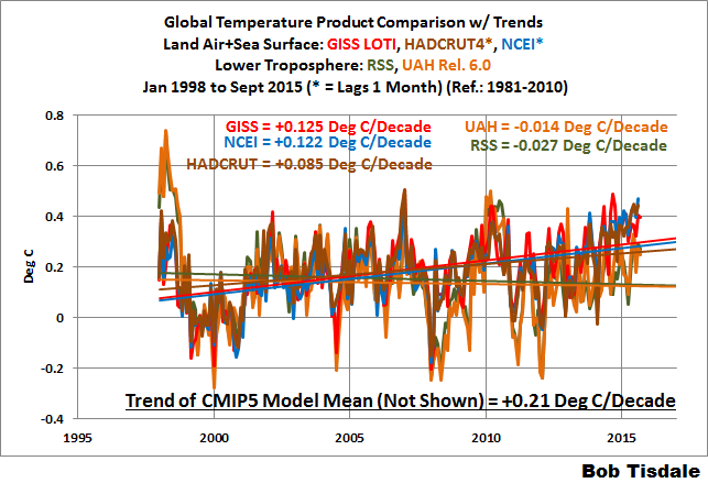
Figure 7 – Comparison Starting in 1998
#####

Figure 8 – Comparison Starting in 2001
Note also that the graphs list the trends of the CMIP5 multi-model mean (historic and RCP8.5 forcings), which are the climate models used by the IPCC for their 5th Assessment Report.
AVERAGES
Figure 9 presents the average of the GISS, HADCRUT and NCEI land plus sea surface temperature anomaly reconstructions and the average of the RSS and UAH lower troposphere temperature composites. Again because the HADCRUT4 and NCEI products lag one month in this update, the most current average only includes the GISS product.

Figure 9 – Averages Surface Temperature Products Versus Average of Lower Troposphere Temperature Products
MODEL-DATA COMPARISON & DIFFERENCE
Note: The HADCRUT4 reconstruction is now used in this section. [End note.]
Considering the uptick in surface temperatures in 2014 (see the posts here and here), government agencies that supply global surface temperature products have been touting record high combined global land and ocean surface temperatures. Alarmists happily ignore the fact that it is easy to have record high global temperatures in the midst of a hiatus or slowdown in global warming, and they have been using the recent record highs to draw attention away from the growing difference between observed global surface temperatures and the IPCC climate model-based projections of them.
There are a number of ways to present how poorly climate models simulate global surface temperatures. Normally they are compared in a time-series graph. See the example in Figure 10. In that example, the UKMO HadCRUT4 land+ocean surface temperature reconstruction is compared to the multi-model mean of the climate models stored in the CMIP5 archive, which was used by the IPCC for their 5th Assessment Report. The reconstruction and model outputs have been smoothed with 61-month filters to reduce the monthly variations. Also, the anomalies for the reconstruction and model outputs have been referenced to the period of 1880 to 2013 so not to bias the results.
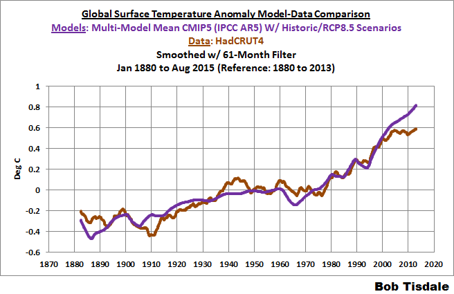
Figure 10
It’s very hard to overlook the fact that, over the past decade, climate models are simulating way too much warming and are diverging rapidly from reality.
Another way to show how poorly climate models perform is to subtract the observations-based reconstruction from the average of the model outputs (model mean). We first presented and discussed this method using global surface temperatures in absolute form. (See the post On the Elusive Absolute Global Mean Surface Temperature – A Model-Data Comparison.) The graph below shows a model-data difference using anomalies, where the data are represented by the UKMO HadCRUT4 land+ocean surface temperature product and the model simulations of global surface temperature are represented by the multi-model mean of the models stored in the CMIP5 archive. Like Figure 10, to assure that the base years used for anomalies did not bias the graph, the full term of the graph (1880 to 2013) was used as the reference period.
In this example, we’re illustrating the model-data differences in the monthly surface temperature anomalies. Also included in red is the difference smoothed with a 61-month running mean filter.

Figure 11
The greatest difference between models and reconstruction occurs now.
There was also a major difference, but of the opposite sign, in the late 1880s. That difference decreases drastically from the 1880s and switches signs by the 1910s. The reason: the models do not properly simulate the observed cooling that takes place at that time. Because the models failed to properly simulate the cooling from the 1880s to the 1910s, they also failed to properly simulate the warming that took place from the 1910s until 1940. That explains the long-term decrease in the difference during that period and the switching of signs in the difference once again. The difference cycles back and forth, nearing a zero difference in the 1980s and 90s, indicating the models are tracking observations better (relatively) during that period. And from the 1990s to present, because of the slowdown in warming, the difference has increased to greatest value ever…where the difference indicates the models are showing too much warming.
It’s very easy to see the recent record-high global surface temperatures have had a tiny impact on the difference between models and observations.
See the post On the Use of the Multi-Model Mean for a discussion of its use in model-data comparisons.
MONTHLY SEA SURFACE TEMPERATURE UPDATE
The most recent sea surface temperature update can be found here. The satellite-enhanced sea surface temperature composite (Reynolds OI.2) are presented in global, hemispheric and ocean-basin bases. We discussed the recent record-high global sea surface temperatures in 2014 and the reasons for them in the post On The Recent Record-High Global Sea Surface Temperatures – The Wheres and Whys.
I have put my money where my mouth is and time will prove if I am right or wrong. I do not have some wishy washy theory with all kinds of outs and excuses.
As for the “either or” … I disagree. It can easily be both and that’s what the Scafetta model attempts to quantify. Scafetta concludes that the GHG forcing is only about 35% of what climate modellers claim. So he then uses 35% of their forecast over-laid on top of harmonic solar model. IMHO, the combined approach is the most robust and most likely to be successful going forward. Statistically, I find it implausible to completely discount all GHG warming. I also find it impossible to justify IPCC climate sensitivity values (around 3.0).
I could be wrong. Scafetta could be wrong. The IPCC could be wrong. Scafetta gets a great fit to past data and is working so far on out of sample data. We will see how it does going forward.
That is his opinion. Time will tell.
I am in a wait and see mode.
No, you are in a personal opinion carpet-bombing mode that nobody needs.
Thanks, Bob Tisdale, for a clear and wide look at the data.
Please keep on doing your excellent work!
Bob, I read your cited piece on the calculation of anomalies. If I understand it correctly, it seems that anomalies are being calculated incorrectly. If the point is to normalize the temperature changes to remove the effects of elevation of the stations, then it seems to me that anomalies should be calculated for every station and then the anomalies should be averaged for a regional or hemispheric average anomaly. Alternatively, if the lapse rate is known for every day at every station, then temperatures could be adjusted to a constant elevation. As it is, it seems to me that all that is being done is to do a 30-day smoothing on the daily readings (high and low elevations) and then calculate a monthly anomaly for stations at different elevations with different lapse rates. Did I miss something?
Why is Dr. Svalgaard (solar scientist from the Stanford University) promoting bad science ?consequence of which could be death of the astronauts which may travel to Mars.
NASA is currently actively planning the manned visit to Mars.
One of the major obstacles is protecting astronauts from deadly cosmic rays not only during travel but also while on the Mars, which has only weak magnetic field.
Here on the Earth we are protected from this deadly radiation by the Earth’s magnetic field.
In his comment HERE Dr. Svalgaard is suggesting that the main and sole protection from the cosmic rays, outside the earth’s atmosphere, is the solar activity, better known as sunspot cycles, result of which is the modulation of the C14 deposition.
On number of occasions I have reminded Dr. Svalgaard, and yet again most recently HERE that it is the Earth’s magnetic field, the strongest modulator of cosmic rays, as well as the principal protector from deadly GCR’s effects on the living organisms.
It is the time that DR. Svalgaard recognises he accepts he is wrong, but if he knows he is wrong, to restrain from publishing misleading information.
The steady galactic cosmic ray flux is not lethal [ask the Inuits living in the Arctic not screened from those]. What we need to protect against is solar cosmic rays caused by transient [and difficult to predict] solar activity.
Astronauts on future deep-space missions farther away from Earth — to Mars or the asteroid belt, for example — face peril from this space radiation. “Galactic cosmic rays don’t reach the surface of the Earth because the planet’s magnetosphere protects us,” Limoli (Charles Limoli, a radiation biologist and neuroscientist at the University of California) said. “It’s one reason why we have life on Earth.”
Astronauts aboard the International Space Station are safe from galactic cosmic rays because they are still protected by the Earth’s magnetosphere, which reaches about 35,000 miles (56,000 kilometers) above Earth’s surface on the day side. (www.space.com)
At high latitudes the galactic cosmic rays are not screened by the geomagnetic field.
What high latitude?
Number, please.
Dr. S.
“At high latitudes the galactic cosmic rays are not screened by the geomagnetic field.”
“ask the Inuits living in the Arctic not screened from those”
Is this high altitude well below average hight of an Inuit ?
What high latitude? Number, please.
A good number for the latitude is 50 degrees.
Everybody who knows anything about this knows that, for the rest you can educate yourself by reading http://www.issibern.ch/PDF-Files/Spatium_11.pdf and look at Figure 8:
“At high latitudes the cosmic ray flux levels off, since the shielding effect of the Earth’s atmosphere becomes larger than the cosmic ray cut-off by the magnetic field”
I apologise to both the GCR impacted Inuits and Dr.S.
I read and wrote the comment without my glasses, and misread latitude for altitude, at least I had good laugh.
Still Dr. S is to very, very large extent wrong; very, very few GCR.s hit poor Inuit, most are absorbed by Oxygen and Nitrogen molecules at high altitudes producing some electrons, gamma rays and of course neutrons, hence neutron count as a proxy for GCR’s.
http://www.americaspace.com/wp-content/uploads/2014/11/cascade-360×408.gif
http://www.americaspace.com/?p=71721
As you can see, only an Inuit taller than 14 km might be exposed to the blast of cosmic rays, that the Earth’s magnetic field was unable to stop.
oops! wrong image. I think this one is good
http://solarphysics.livingreviews.org/Articles/lrsp-2013-1/LR_cascade.png
Many more Here
None of those show the screening by the magnetic field, only by the air in the atmosphere.
Good grief man!
This is from the online library of one Dr. L. Svalgaard
http://www.leif.org/research/CosmicRays-GeoDipole.jpg
Title of the link is CosmicRays-GeoDipole
I have saved it in case you remove it.
Shows very nicely the effect of the geomagnetic field which , of course, is removed when the solar modulation is computed.
lsvalgaard
“At high latitudes the galactic cosmic rays are not screened by the geomagnetic field.”
“the geomagnetic field which , of course, is removed when the solar modulation is computed.”
C14 data comes from Greenland and Antarctica, places at high latitudes
Effect of magnetic field is removed first to extract C14 data
Astronauts are not at travelling to Mars at high latitudes, last time I looked at Mars orbit is just outside the Earth’s equatorial plane.
I’ll say again : good grief man.
Some less informed reader may believe to your statements and impeccable contradictions.
CASE CLOSED.
C14 data comes from Greenland and Antarctica, places at high latitudes
Yeah, from all the trees that grow there…
“Yeah, from all the trees that grow there…”
Being snarky doesn’t contribute to understanding the claims and counter-claims. There is plenty of en-trained air in glacial ice, not to mention dust and soot. When I was in the army I was stationed at the Cold Regions Research and Engineering Laboratory. I supervised a survey crew doing a closure survey on a tunnel driven into the snout of the Greenland glacier. We were frequently interrupted by Danish pilots doing ‘Blue Bird flights’; they would show up with stewardesses and chip clean ice out of the walls of the tunnel to use to make mixed drinks later at cocktail parties. They did so because they thought that the fizzing ice was quite a novelty.
Does not change the fact that the 14C cosmic ray proxy is constructed from trees grown elsewhere.
… and ice cores for 10Be deposits, which is a bit more but not much reliable cosmic rays proxy.
remember we are discussing Cosmic Rays, not C14 alone.
As Slide 6 [bottom panel] of http://www.leif.org/research/The%20long-term%20variation%20of%20solar%20activity.pdf shows, 10Be and 14C proxies agree very well.
10Be From the ice cores of the tree-less high latitudes
Changes in the cosmic ray…McCracken (2007)
“This paper first presents the inter-calibrated cosmic ray record for 1428–2005, as determined record in Fig. 1 was calculated using the Climax neutron monitor record 1951–2005: the ground level and high altitude ionization chamber record, 1933–1954; and the 10Be concentrations observed in central Greenland, 1428–1932. by McCracken and Beer (2007).
The data have been adjusted to remove the effects due to the long-term change in the
geomagnetic dipole.
9,400 years of cosmic radiation ….Steinhilber et al (2012)
We combined a new 10Be record from Dronning Maud Land, Antarctica, comprising more than 1,800 data points with several other already existing radionuclide records (10Be analyzed in polar ice cores of Greenland and Antarctica) covering the Holocene.
“Note that the variation on the millennial time-scale of F depends on the geomagnetic field.
First, we reconstructed the solar modulation potential, which is a measure of the solar modulation of the cosmic ray particles by removing the effect of the geomagnetic field based on paleomagnetic data reconstructed in Knudsen MF, et al. (2008)”
Do you still hold (grossely distorted) view that
“At high latitudes the galactic cosmic rays are not screened by the geomagnetic field.” ?
the 10Be found at high latitudes is not generated there, but over the much larger area low and mid-latitude regions [where the cosmic rays are screened] and brought up to the polar regions by atmospheric circulation.
The dependence on the geomagnetic field is characterized by the so-called cut-off energy which is the energy determining which cosmic rays are screened by the magnetic field. At low latitudes that energy is of the order of 10 GeV, decreasing to 0 GeV [i.e. no screening] at high latitudes. E.g. at Thule as McCracken reminds us in “Fig. 4. The observed cosmic ray ionization versus atmospheric depth at Thule, Greenland, where all cosmic rays gain access down to the height dependent atmospheric cutof”
http://ftp.issibern.ch/teams/Variable/Referencepapers/McCrackenetalASR2004.pdf
This is well-known [has been for almost a century] by people who know what they are talking about.
Here is an early graph showing this ‘latitude effect’
http://www.leif.org/research/GCR-Latitude-Effect.png
As you can see, above about 50 degrees there is no significant ‘screening’. I pointed that out to you earlier, but you [as we all know] are a self-professed slow learner.
http://www.onafarawayday.com/Radiogenic/Ch14/Ch14-3_files/image006.jpg
Ah, it seems that you have learned something, after all. The screening is largest at the equator and falls to zero at the poles thus the maximum cosmic rays per unit area is at the poles, but the area is largest at the equator and dwindles to zero at the poles. The combined effect is that somewhere in between the concentration will be largest as your plot shows. Congratulations for having understood something.
A better picture is this one from the textbook Cosmogenic Radionuclides by Beer, McCracken, and von Steiger Figure 13.4-2 on page 218:
http://www.leif.org/research/10Be-Production-Deposition.png
The black curve is the production rate. Note that the geomagnetic screening only becomes effective below latitude 60 degress. The red curve is the deposition rate.
The authors note [page 222] that
“changes in solar activity cause much larger production variations than near the equator, while changes in the geomagnetic field result in large production changes at low latitudes, and no effect whatsoever in the polar regions.
From this it would appear that an archive in the tropics would be ideal to study the history of the geomagnetic fields, and one near the poles to study solar activity in the past. However, examination of the transport processes has provided a completely different picture. The atmosphere is a highly dynamic system consisting of a thermally driven troposphere with three large convection systems in both hemispheres with residence [of 10Be] times ranging from a few days to several weeks, and a rather stratified stratosphere with residence times of a few years. […] As a consequence of these dynamic processes, there is substantial mixing of the atmosphere with the result that the flux of 10Be into a polar archive is rather well mixed, and the production signal imprinted on 10Be by the sun and the geomagnetic field is close to the global average. […] In addition, for long time scales […], climate change may affect the atmospheric circulation. As a result, the local deposition fluxes may change without any changes in the production rate.”.
So, as you can perhaps see, the situation is complex, but is also well-understood.
…larger production variations in the polar regions than…
Thus we have to conclude this is wrong because doesn’t take into account decadal changes in the Earth’s magnetic field (at equator or elsewhere)
http://www.leif.org/research/Comparison-GSN-14C-Modulation.png
And this shows that correct decadal changes in the Earth’s magnetic field should be accounted for
http://www.vukcevic.talktalk.net/GMF-C14.gif
When you come back with an answer to one or more of the following:
– why gmf changes are more or less concurrent with solar activity, but are two orders of magnitude stronger than the heliospheric magnetic field at the Earth’s orbit ?
– are these changes induced by solar activity ?
– is there a common cause ?
as stated at the beginning of this dialog, I would be interested to hear.
The obfuscations and diversions (including ad hominem) from fundamental questions are of no interest to me, perhaps are to the other readers so you are welcome to continue..
Bye
1) The plot is not wrong. In calculating the modulation potential, the changes in the geomagnetic dipole has been fully accounted for.
2) Your curve does not show the change in the dipole moment, so your question is moot.
http://www.leif.org/research/Earth-Dipole-Moment.png
The surface is not of interest as the geomagnetic field is generated in the core [where it is much stronger] and cannot be influenced by the solar wind.
And scientific dishonesty is to remove the part of the curve that shows failure as you did here
http://www.vukcevic.talktalk.net/MV-DrS.gif
Shame on you.
My plot shows exactly what it says.
Knudsen and some other dipole data use excessive filtering or smoothing.
Try using Korte’s CALS3k.4 dipole data, then calculate 22 year delta
Ah.., yes magnetic field generated at core and having 22 year quasi-periodic oscillations you hate to be reminded of.
http://www.vukcevic.talktalk.net/SSN-GMFc.gif
Alternatively you can use IGRF geo-polar data, no less inconvenient than one shown above.
http://www.vukcevic.talktalk.net/GT-GMF1.gif
There is no escape, solar activity, geomagnetic field and climate change are linked together directly or indirectly by a common cause, and as a scientist you could take a sceptical position, but denying the existence of the link is a dogmatic stance, and as such the good science doesn’t tolerate it.
It is not bad science to say we don’t know, but it is bad science to say “it is impossible”.
There are laws of physics that determine what is possible. And here is the actual variation of the dipole:
http://www.leif.org/research/Earth-Dipole-Moment.png
http://www.leif.org/research/Earth-Dipole-Moment-No-Trend.png
based on actual measurements (data, you know) without smoothing and manipulation.
what is that? what are your units? As John McEnroe said: “You must be joking, man”
NOAA’s IGRF (N+S) data are shown in my graph above (blue line) .
The dipole is around 30 uT [or 30,000 nT], not the 125 uT that you use.
But the unit for the dipole moment is Ampere/m^2 as shown on my plots. The lower plot is just the detrended down version of the upper right plot [simply tilted]. Note that for 1830 the value is the same as for 2000.
Here is reminder how to calculate geomagnetic dipole
Geomagnetic poles are not same as the geographic or magnetic poles
These two images give locations (marked by blue lines)
http://www.geomag.bgs.ac.uk/images/polesfig1.jpg
http://www.geomag.bgs.ac.uk/images/polesfig2.jpg
While magnetic poles have travelled some distance in the last 100 years, geomagnetic poles moved very little. For simplicity of calculation you can use mid-location, but if more adventures there are tables showing accurate coordinates.
Now, you estimated (or calculated) latitude and longitude for each location
Go to NOAA’s geomagnetic calculator
http://www.ngdc.noaa.gov/geomag-web/#igrfwmm
– enter your coordinates
– select IGRF,
– enter period of interest (I use 0 km, since that is most relevant to the climate events, since oceans happen to be on the earth’s surface not up in the exo-sphere)
– select CSV (the Excel –ready) and hey presto
– column 5 gives values for total intensity for each geomagnetic pole.
As with any other magnetic entity, the dipole strength is sum of intensity at each pole, and since ours happen to be geomagnetic poles calculated sum represent geomagnetic dipole.
Now you can show result of your calculations not as a ‘shaggy dog’ but a proper graph so the readers see what is actually happen with geomagnetic dipole.
To compare to global temperature y scale needs to be inverted.
Result:
http://www.vukcevic.talktalk.net/GT-GMF1.gif
That might take you some time, so I am off elsewhere for a while.
That is not how the dipole is calculated [and is not how you did it with CALS3k.4] The correct way is use the g01 component of the spherical harmonics that describe the main field. Done right, you would get:
http://www.leif.org/research/Earth-Dipole-Variation-Korte.png
which blows your spurious correlations out of the water.
p.s. For next project (will leave it for tomorrow) I will post again a simple guide how to reproduce this:
http://www.vukcevic.talktalk.net/SSN-GMFc.gif
Try using Korte’s CALS3k.4 dipole data, then calculate 22 year delta Ah.., yes magnetic field generated at core and having 22 year quasi-periodic oscillations
Korte’s CALS3k.4 data has a time-resolution of 10 years, so is not suitable for detecting 22-yr oscillations [and BTW does not have them].
“which blows your spurious correlations out of the water.”
No it does not, my geomagnetic dipole calculation shows good agreement with Calsk3k.4 and Calsk 7k.2
http://www.vukcevic.talktalk.net/GMF-Ds.gif
Now be brave, invert your de-trended dipole shift to the right by a decade, de-trend CruTem4 and compare !
No it does not, my geomagnetic dipole calculation shows good agreement with Calsk3k.4 and Calsk 7k.2
No it does not:
http://www.leif.org/research/Vuk-Failing-30.png
Complete failure.
I already showed you the detrended variation and will you gloat over how well it fits. Especially about the temperature in the early 19th century:
http://www.leif.org/research/Earth-Dipole-Variation-Korte.png
A sure sign of a spurious correlation is that it fails outside of the interval on which it was claimed, like here:
http://www.leif.org/research/Vuk-Failing-31.png
Big failure before 1850
“Korte’s CALS3k.4 data has a time-resolution of 10 years”
GUFM1 and NOAA do, use Greenland for Greenland ice cores.
The higher resolution comes from interpolation and is not real data. And you did claim you used Korte, so you just lied and hoped that nobody would notice…
I plotted the main dipole component g01. One gets a sharper definition by calculating the magnitude of an eccentric, non-centered dipole including the higher harmonics g11 and h11: SQRT(g01^2+g11^2+h11^2).
This is shown by the cyan curve. The variation from the linear mean is almost the same [brown symbols] as that from the simpler g01 variation [yellow symbols]. So the higher harmonics don’t change the conclusion.
Now, this is the surface field. The core fields look rather different and it is somewhat meaningless to assume the surface variation is the same as the core variation.
And you did claim you used Korte, so you just lied and hoped that nobody would notice
NO I DID NOT
What I said is here
http://wattsupwiththat.com/2015/10/14/september-2015-global-surface-landocean-and-lower-troposphere-temperature-anomaly-model-data-difference-update/#comment-2051727
as clear as daylight:
“Knudsen and some other dipole data use excessive filtering or smoothing.
Try using Korte’s CALS3k.4 dipole data, then calculate 22 year delta”
Since you didn’t trust my data I suggested to use widely accepted Korte’s data.
I doubt that you would apologise or withdraw your comment, but that is something you should worry about, resorting to that kind of discussion is more akin to AGW alarmists, when loosing argument, only insults left in your armoury.
Data is the only weapon of my argument
Wiggle, wriggle, nonsense, and nasty ad hominem
I shown 7k.2 geopolar dipole from Korte’s 7k.2 data, good match
Korte’s 3k.4 data has different values and when those used then geopolar dipole matches Korte’s 3k.4 dipole
Now you have confirmed by yourself that geomagnetic dipole, as calculated by yourself , is confirming my findings, that geomagnetic dipole and global temperatures are highly correlated (Svalgaard – yellow line)
http://www.vukcevic.talktalk.net/MV-DrS.gif
(failure before 1850 is not much concern to anyone, since we have no global temperature data) I am going regularly promote your graph, so get your dictionary of unpleasant insults on the ready.
vukcevic October 19, 2015 at 1:11 am
And you did claim you used Korte…
NO I DID NOT
Your wording strongly suggests that you did. Now you are trying to wiggle out of that, but credibility once lost is hard to regain.
I shown 7k.2 geopolar dipole from Korte’s 7k.2 data, good match
Not at all. Dismal failure as I showed. Now, the dipole is by far the strongest component, so even your crude [and basically wrong] method will give a rough indication of the dipole, but it should be calculated correctly as I did.
(failure before 1850 is not much concern to anyone, since we have no global temperature data)
Not so. Your ‘correlation’ ‘predicts’ a temperature during the Dalton minimum [with its ‘year without a summer’] to be as high as the latest years which are the warmest ‘ever’. There are lots of data for the Dalton minimum, e.g. CET, and Loehle, Moberg, and BEST. All showing the colossal failure of your correlation:
http://www.leif.org/research/Temps-1800-1850.png
As I said: scientific honesty is not to cling to something that has been roundly falsified.
No one is certain either of magnetic field data (Gauss invented magnetometer/graph in 1833, there are no even reasonable temperature data before 1850. No one cares much of what happen before 1850, since there is hardly any agreement post 1850.
What I wrote and what your impressions are are two different things. In such case some people would apologise but I don’t ask or expect it from you, you stepped over the line too many times.
No one cares much of what happen before 1850
Especially not the one whose pet hypothesis is falsified by what happened before 1850.
Both the magnetic data and the temperature data are well constrained at least back to 1800 as I showed.
What is disturbing and telling is that you removed the part of the curve that didn’t fit your correlation:
http://www.leif.org/research/Vuk-Failing-32.png
Scientific dishonesty.
Scientific dis-honesty, or really? What next?
It suits your argument to use period of dodgy proxies of the pre-instrumental data.
It suits my argument to use only the period of instrumental data.
What is disturbing is that you as a scientist in the field assume that there are any accurate measurements of magnetic field intensity before magnetometer was invented in 1833. It might have taken a decade or two before it was in a wider use at least in half a dozen locations around 360 degrees of N. Hemisphere’s longitude from Europe, Russia, Chine and Japan to the west and east coast of America.
If you think that there are any good global temperatures data before 1850, I’d say ‘do keep believing’.
165 years of correlation with instrumental data is what matters !
I’ll repeat: Svalgaard of Stanford University (accidentally) confirmed Vukcevic’s finding that since 1850 (wider availability of instrumental records) global temperatures are correlated to the changes in the Earth’s magnetic field.
Now he is at some pain to deny importance of his confirmation (unfortunately too late) by calling onto the dodgy proxies for both magnetic field and in particular double-dodgy proxies for the global temperatures before 1850.
It is satisfactory state of affairs when the most bitter opponent of the hypotheses unintentionally confirms it, while he/she is trying to invalidate it.
any accurate measurements of magnetic field intensity before magnetometer was invented in 1833.
Gauss did not need to rely on any such measurements so your assertion is baseless. Here is his original publication [in translation]:
http://www.leif.org/EOS/GaussMagnetic2.pdf
He used the total intensity map produced by Sabine from observations all over the globe in the 1820s. At the time intensity was measured in Humboldt Units determined by measuring the number of swings of a magnetic in 5 minutes [the stronger the field, then fewer swings]. Was Gauss managed to do was to determine the what the Humboldt unit was in absolute terms [meter-kilogram-second units].
Your removal of the data before 1850 is typical of your scientific dishonesty. What more needs to be said?
I order to affirm your scientific honesty , you should not be ignoring but bringing to the readers attention, that your own average of sunspot group numbers from 1820 to 1850 was commensurate with those 1950 and 2000
http://www.leif.org/research/Comparison-GSN-14C-Modulation.png
Most of us think or even know, and you are at pains to deny, that the global temperature change is controlled by the sun, but the earth’s and solar magnetic field (as Vukcevic has shown) are in strong contra-correlation. We just don’t know why is this.
Go on, affirm your scientific honesty, sir
I think that the Figure shows just that which contradicts your claim that the sun is a major driver of climate, c.f. http://www.iau.org/news/pressreleases/detail/iau1508/
Most of us think or even know
“It is not what you ‘know’ that gets you in trouble, but what you know that ain’t so”
‘know’ is not science, but belief.
Svalgaard is wrong !
Only weapons in his armoury left are insults
His insensate rattling on about failure before 1850 has become more than tedious, but he failed to realise that Vukcevic is ‘good’ for another 200 years, all the way back to 1650.
Vukcevic kept this for his final parting shot
http://www.vukcevic.talktalk.net/LLa.gif
Good doc has embarrassed himself far too many times.
First you claim that both the magnetic field and the temperatures are junk before 1850. Now you claim they prove you right. This is not science, but rhetoric.
And your delta Bz is junk. You claim the dipole is the driver. So here is the 20-yr changes of the dipole:
http://www.leif.org/research/Change-Dipole-20-yrs.png
Does not correlate with temperature. Your claim is no good. But you keep throwing mud, hoping some will stick. Unfortunately none of it does.
It is amusing, actually, to watch your antics.
ps. Svalgaard is misleading readers, although there are some measurements in the N. Hemisphere, to calculate the dipole an equal amount of measurements from S. Hemisphere is required, but they do not exist!
Nevertheless, you use that non-existing data for your curve.
But the dipole does not need such measurements to be determined. Measurements at only one place are needed.
The formula for a dipole field B over a sphere is B = M sqrt(1+3cos^2(q))/r^3
where M is the dipole moment, r the distance from the center, and q the colatitude. Measure B at a place with colatitude q and the dipole moment M is known. If the dipole is not centered, you need only three measurements at three different places not necessarily in opposite hemispheres.
I am in very strong agreement with you vuk on that point.
http://www.express.co.uk/news/weather/612369/SHOCK-CLAIM-World-is-on-brink-of-50-year-ICE-AGE-and-BRITAIN-will-bear-the-brunt
My thinking to one degree or another. As I said it is a wait and see mode and see how it all plays out.
Say, I’m a climate modeller. Nothing I have forecast
or hindcast in the past has eventuated and everything
I have projected and extrapolated and published in pal-
reviewed journals has been falsified by real-world data.
But trust me and send more grant money – for I am a
climate modeller.