Guest essay by Jim Steele
Reference link: Déformation professionnelle
Director emeritus Sierra Nevada Field Campus, San Francisco State University and author of Landscapes & Cycles: An Environmentalist’s Journey to Climate Skepticism
For the past 55 million years the global surface temperature has declined by more than 10°C from a “hot house” condition into an “ice house” with increasing temperature variability as depicted in Figure 1 (Mya = millions of years ago). During the Cretaceous and Early Cenozoic, glaciers and ice caps were absent from both Antarctica and Greenland. Antarctica was covered in para-tropical vegetation and Greenland was home to crocodiles. More importantly for millions of years the oceans had been storing enormous amounts of heat. In contrast to near freezing temperatures today, Antarctic bottom waters averaged about 11°C, suggesting Antarctic coastal temperatures never dropped below 11°C even during the long polar nights. Amazingly the equator to pole surface temperature difference averaged just 10°C compared to the 30°C gradient measured today. Of particular interest, changes in carbon dioxide fail to explain the greatest proportion of these ancient temperatures.

For decades the consensus had been that ocean heat transport had ultimately maintained the polar regions’ ancient tropical conditions. Models had demonstrated without heat transport from the tropics, the poles would be 110°C colder than the tropics (Gill 1982, Lozier 2012). It was commonly believed, and is still believed by most, that as plate tectonics rearranged the continents, the Antarctic Circumpolar Current (ACC) formed and strengthened. Models now simulate that as drifting continents opened “gateways” and allowed for uninterrupted circumpolar flow, surface temperatures began cooling significantly (Bijl 2013). A strengthening ACC created a barrier inhibiting intrusions of warm tropical waters and minimizing both oceanic and atmospheric heat transport resulting in the Refrigerator Effect. The Refrigeration Effect radically cooled the southern ocean and altered the vertical temperature structure of all the earth’s oceans. (As discussed here, the ACC barrier to ocean heat transport is a major reason why Antarctic sea ice has currently increased in contrast to decreasing Arctic sea ice.)
However a few climate modelers began arguing CO2, not heat transport, was the ultimate climate control knob. They argued that high CO2 concentrations explained the polar warmth and the decline in CO2 explained the advent of polar ice caps and the 55 million year trend towards our icehouse climate. This debate between heat transport and greenhouse effects not only reveals a lack of climate consensus; it also reveals the subjectivity that influences how climate sensitivity is estimated. Proxy evidence increasingly suggests that ancient CO2 levels were far lower than what climate models require to simulate ancient warmth. In stark contrast to current research that is increasingly suggesting lower climate sensitivity to CO2 (i.e. Lewis & Curry 2014, and a growing list here and here), paleoclimate researchers who argue CO2 controls climate change, are forced to suggest climate sensitivity must have been much, much greater than anyone currently believes.
In contrast, researchers examining the Paleocene‑Eocene maximum temperatures concluded, “At accepted values for the climate sensitivity to a doubling of the atmospheric CO2 concentration, this rise in CO2 can explain only between 1 and 3.5°C of the [5-9°C] warming inferred from proxy records. We conclude that in addition to direct CO2 forcing, other processes and/or feedbacks that are hitherto unknown must have caused a substantial portion of the warming during the Paleocene–Eocene Thermal Maximum. Once these processes have been identified, their potential effect on future climate change needs to be taken into account.” [Emphasis added] Zeebe (2009).
However if “unknown feedbacks” and other forcings can explain an even greater proportion of past temperature changes, then researchers would be forced to suggest climate sensitivity to CO2 is much lower. The Antarctic Refrigerator Effect is such an effect and parsimoniously explains Cenozoic global cooling without invoking a CO2 contribution.
The Case Against a CO2 Climate “Control Knob
By creating a well‑mixed global “blanket”, the carbon dioxide greenhouse effect should act on a global scale. However as illustrated in Figure 1, initiation of Antarctic glaciation happened 35 million years ago, more than 30 millions years before Arctic glaciation ever began. Clearly Antarctic glaciation was not part of a global event, but a regional one. Although this gross time difference does not rule out a limited contribution from diminishing CO2 concentrations, the evidence most assuredly demands a different and more regional explanation for the drivers of Antarctica’s observed climate change.
Furthermore, in order for a CO2 greenhouse effect to have created the near‑tropical conditions observed in Antarctica’s fossil evidence, it requires CO2 concentrations far greater than what the growing number of paleo‑proxies are suggesting. Huber (2011) argued that their models could simulate tropical warmth in polar regions if CO2 reached 4480 ppm, an 11‑fold increase above today’s concentrations. However Huber 2011 also admitted their estimate of CO2 concentrations should not be taken literally. Instead it was his approach “equivalent to “tuning” climate sensitivity to a higher value, but is much simpler in practice.” They argued that the “4480 ppm CO2 concentration used here should not be construed literally: it is merely a means to increase global mean warmth.”
Huber 2011 was wise to admit CO2 concentrations of 4480 are unrealistic. Based on growing proxy evidence, CO2 concentrations during the past 350 million years have not exceeded 1000 ppm (Franks 2014). However Huber 2011’s suggestion of greater CO2 climate sensitivity proves to be equally inappropriate and most likely a case of déformation professionnelle.
Deformation professionnelle is a French term referencing how one’s profession narrows and distorts one’s viewpoint and thus biases conclusions. For example if researchers whose funding and status has been driven by a paradigm that CO2 drives all climate change, any contrary evidence will be reinterpreted to maintain that viewpoint.
One major avenue of research strives to determine climate sensitivity by comparing varying CO2 concentrations with past climate change. Although Franks 2014 determined past CO2 variations only accounted for 20% of what Huber’s models required, they too felt obligated to suggest there must be a much greater climate sensitivity to the smaller changes in CO2. But they obviously ignore much more parsimonious inferences. Very simply, there are other dynamics that drive climate change, and current models driven by CO2 have failed to incorporate additional and alternative explanations. Similarly CO2 variations are insufficient to explain the Dansgaard‑Oeschger extreme warming events of the last Ice Age. But as discussed here, changes in ocean heat storage and ventilation offer a superior explanation. Likewise Antarctica’s Refrigerator Effect completely altered ocean heat storage and ventilation and can parsimoniously accounts for Cenozoic global cooling.
Unfortunately evaluations of CO2 climate sensitivity typically only compare varying CO2 concentrations with other estimated radiative effects to explain fluctuations in global mean surface temperatures (GMST). However there are other powerful non-radiative effects that also contribute to a varying GMST as well as the increasing equator to pole temperature gradient. For example examining changes in Cenozoic climate Thomas (2014) concluded, “Stronger vertical mixing within the oceans potentially reconciles several long-standing greenhouse paleoclimate problems. Stronger vertical mixing invigorates the MOC [Meridonal Overturning Circulation] by an order of magnitude, increases ocean heat transport by 50–100%, reduces the zonal mean equator-to-pole temperature gradients by up to 6°C, lowers tropical peak terrestrial temperatures by up to 6°C, and warms high-latitude oceans by up to 10°C.”
Given that just the upper 3.5 meters of the oceans hold more heat than our entire atmosphere. And that average depth of the oceans is an order of 3 magnitudes greater, about 3600 meters; changes in ocean heat storage and ventilation have humongous impacts on global climate. Research that ignores contributions to GMST from ocean heat storage, ventilation and vertical mixing, CO2, will greatly exaggerate climate sensitivity to CO2. Today we witness global warming from heat ventilation during an El Nino and global cooling due to increased upwelling of cooler waters during La Ninas. On time scales varying from a few years to millions of years, storage and ventilation of ocean heat has been the earth’s true climate control knob.
The Antarctic Refrigeration Effect
Our modern freezer and refrigerator appliances are all based on 2 simple principles. 1) A compressor‑refrigerant apparatus pumps heat out of the refrigerator’s interior. 2) The refrigerator is insulated to minimize any heat transfer into the refrigerator from the outside.
The Antarctic analogy to a refrigerant/compressor apparatus has been ever present. Due to the earth’s spherical shape and orbital effects, annual incoming solar radiation at the poles is so low, polar regions always radiate more heat back to space than is ever absorbed locally. Without a constant flow of heat from the tropics, polar regions would naturally descend into permanent ice house climates. Forcing by CO2 is not a significant factor, if a factor at all. Thus variations in Antarctica’s climate are governed by changes in heat transport versus the steady radiation of heat back to space. Although Antarctica sat over the South Pole for hundreds of millions of years, it remained ice free for most of the Mesozoic and early Cenozoic because the “refrigerator door” was left open. However as continents began to shift and opened “ocean gateways”, the Antarctic Circumpolar Current (ACC) formed and intensified. The ACC closed the refrigerator door and resisted poleward heat transport from the tropics. The ACC also generated more intense westerly winds and invigorated upwelling that increased vertical mixing. Most importantly as the ACC shut the refrigerator door, sea ice began forming in the southern seas. That initiated deep ocean cooling and a total reconfiguration of the global ocean’s vertical heat structure.
Before the ACC formed, Antarctic bottom waters were about 11°C. Bottom waters formed from competing regions. In shallow seas that dominated subtropical regions, warm salty water became dense enough to sink to the bottom. Elsewhere warm salty subtropical waters that were transported poleward cooled and sank. In contrast, once the Antarctic refrigerator was established, cold salty brine was now extruded during sea ice formation. The sinking of cold brine either penetrated to the abyss forming near freezing bottom water, or slowly cooled the subsurface waters as the brine was turbulently mixed with its surroundings. Thus global oceans began a 35 million year cooling trend starting from the ocean abyss and working its way to the surface.
In Figure 13 below (from Kennett 1990), the bottom frame labeled Proteus, illustrates a simplified vertical structure of the Atlantic Ocean around 60 million years ago. Warm Salty Deep Water (WSDW) dominated the ocean depths. Much of that warm bottom water is believed to have been generated in shallow equatorial seas, like the Tethys, where evaporation exceeded precipitation. Our modern Mediterranean Sea is a remnant of the Tethys, and still contributes warm salty water to the Atlantic.
The surface waters around Antarctica were much fresher because cooler polar regions experience greater precipitation relative to evaporation. Antarctic Intermediate Water (AAIW) forms as upwelling bottom waters mixed with fresher surface waters. Subsequently, climate change has been greatly affected as Antarctic Intermediate Water have cooled and exerted a tremendous effect on tropical sea surface temperatures for millions of years via “ocean tunneling”.
The middle frame of Figure 13, labeled Proto-Oceanus, illustrates how the ocean’s vertical structure evolved over the next 10+ million years after the formation of a strong Antarctic Circumpolar Current. Due to the refrigerator effect, cold saline Antarctic Bottom Water (proto‑AABW) began to dominate the ocean floor. Contributions of Warm Saline Deep Water (WSDW) diminished, and the influential Antarctic Intermediate Water (AAIW) was increasingly cooled by much colder Antarctic Bottom Water. As the colder AAIW flows back towards the equator it modulates the global temperature by cooling subsurface waters that would potentially reach tropical surfaces via upwelling.

The upper frame labeled Oceanus, represents a simplified illustration of the Atlantic’s modern vertical structure. Due to the Antarctic Refrigerator Effect, the deep oceans continued to cool, and the thermocline that separates warm surface water from cooler deep waters became increasingly more shallow.
Between 2 and 3 million years ago the cooling of the deep oceans reached a tipping point, and modern upwelling regions ogf cold deep water off the coast of Peru, California and the west coast of Africa were established. There had always been upwelling along those coasts along with the associated increases in marine productivity. But now upwelled subsurface waters were cooler by 4 to 9°C. (Dekens 2007), corresponding to the cooling by Antarctic Bottom waters and its effect on subsurface waters. Analogous to the drop in global temperatures during La Nina events caused by upwelling of colder waters, upwelling of colder waters 2 to 3 million years ago also cooled global temperature to the point it initiated Arctic ice cap and glacier formation. The cooler Arctic then promoted formation of North Atlantic Deep Water (NADW in the upper frame of Figure 13) as salty Atlantic waters transported poleward cooled and brine rejection increased as more Arctic sea ice formed.
Declining CO2: A Result Not A Cause.
The Cretaceous Period (145 to 65 million years ago) was named for huge widespread chalk deposits that developed during that time period, especially in the Tethys Sea. Those chalk deposits were the result of sinking plankton that produced calcium carbonate shells like foraminifera and coccolithophorids, As discussed in Natural Cycles of Ocean Acidification, the creation of calcium carbonate shells pumps alkalinity to depth but produces CO2 at the surface thus adding to higher concentrations of atmospheric CO2. More enlightening and contrary to catastrophic CO2 assertions that rising CO2 will decimate calcium carbonate shell producers, the greatest proliferation of calcium carbonate shell producers occurred during this period with the high temperatures and high concentrations of atmospheric CO2. Quite likely, high CO2 concentrations did not produce detrimental acidification, and were the result of coccolithophorids and foraminifera pumping CO2 to the surface.
The development of the Antarctic Circumpolar Current forever altered the carbon biological pump by increasing upwelling in the southern oceans, and later along continental west coasts by cooling upwelled waters. When the ACC caused upwelling in southern oceans to intensify, a more reliable supply of nutrients supported the evolution and proliferation of diatoms. As discussed in Natural Cycles of Ocean Acidification, diatoms are large, produce siliceous shells, and more rapidly shuttle CO2 from the surface to ocean depths. As evolving diatom populations expanded, a more efficient biological pump buried more CO2 at depth that is now detected as siliceous ooze or as biogenic opal deposits. In contrast CO2 emitting coccolithophorid populations and their chalk deposits dwindled. Changes in the biological pump contributed to observed declines in atmospheric CO2. Diatoms are also associated with explosive increases in ocean productivity, so it should be no surprise that the earliest appearance and evolution of whales also coincides with increased ACC upwelling and the evolution of diatoms.
In summary, due to continental drift, the formation of the Antarctic Circumpolar Current blocked intrusions of warm tropical waters that warmed Antarctic and initiated the Antarctic Refrigerator Effect. Cold polar regions are a natural result of inadequate solar radiation. Reduced forcing from diminished levels of CO2 is not required to explain global cooling. The resulting formation of Antarctic sea ice expelled colder, salty waters that filled the abyss and began cooling the deep oceans. After 30+ million years of cooling, 2 to 3 million years ago, colder ocean waters eventually upwelled in the mid latitudes along the west coasts of major continents as well as along the equator. The resulting global cooling, allowed the growth of Arctic ice caps, glaciers and sea ice. The Antarctic Circumpolar Current also increased global upwelling and the efficiency of the biological pump. Decreases in atmospheric CO2 are associated with reductions in populations of CO2 producing coccolithophorids along with increasing populations of diatoms that pumped CO2 to depth. If the Antarctic Refrigeration Effect can account for the changes in global temperatures, it suggests the global sensitivity to varying levels of CO2 is relatively insignificant.
Jim Steele is author of Landscapes & Cycles: An Environmentalist’s Journey to Climate Skepticism

While I agree with this over the long-term,
It does rely on,
Which isn’t operating on the timescales that anyone is worried about in the first place.
It only relies on continental drift as the trigger for the Cenozoic cooling trend. For current timescales the point is storage and ventilation of ocean heat are the control knobs driving climate change, and more ice in the Arctic is not dependent on CO2 forcing, but small changes in iinsolation and heat transport into the Arctic
I’m confusing myself here. Seemingly without the acc warm water could more easily get to the poles for cooling so I’m having trouble seeing where the buildup of heat came from. Maybe decreased albedo and presumably increased water vapor at the poles? Did I miss it in the report?
Certainly it would be interesting to observed the polar weather back then
Tazz, maybe thinking about where Antarctica was at the time helps. It was not at the South Pole 70MYA (or mostly not) and was not much separated from Australia. All the major land masses had big gaps between them and the oceans were deeper as the water was not locked up in Ice Caps, so the circulation of warm water was fairly easy. However, once Antarctica drifs far enough down and away from Australia, the ACC develops and starts to insulate the continent, cooling in Winter and never warming up again in Summer.
I came up with my “saucepan” analogy. When I’m cooking in a large flat pan, if I stir it with a spoon (Think circulation) it is all uniformly heated even though the heat source is only applied to a small area (the Tropics). If I stop stirring (isolate the edge of the pan), the sauce directly over the gas flame can boil, even when the rest of the sauce is cooler (the current situation).
Tazz,
Without the ACC warmer water approaches the poles adding warmth and preventing freeezing temperatures. In the Arctic intruding warm Atlantic waters circulate beneath the Arctic Ocean between 100 and 900 meters and can accumulate until ventilated in interglacials and D-O events or similar warm spikes of the 20th century.
If you are asking how did the oceans warm before the ACC formed, it was due to the sinking of warm salty waters that were free from competition with cold polar water and brine extrusions. Without near freezing waters and brine, the most dense water capable of sining to the bottom was warm salty water, and that is what accumulated during the Cretaceous.
Thanks. I think I’m stuck on how different cretaceous weather was compared to current. Hard to imagine reasonably warm weather when the sun doesn’t come up for weeks.
http://wattsupwiththat.com/2015/09/16/antarctic-refrigerator-effect-climate-sensitivity-dformation-professionnelle-lessons-from-past-climate-change-part-2/
Thank you Jim.
You say in your above section “Declining CO2: A Result Not A Cause:”
“As discussed in Natural Cycles of Ocean Acidification, the creation of calcium carbonate shells pumps alkalinity to depth but produces CO2 at the surface thus adding to higher concentrations of atmospheric CO2.”
I demonstrated in 2008 that dCO2/dt varies almost contemporaneously with global temperature T (Surface Temperature ST and Lower Troposphere Temperature LT) and the integral atmospheric CO2 concentration lags temperature by about 9 months in the modern data record. I believe this short-term “CO2 lags T” relationship is primarily driven by terrestrial biological activity that is dominated by the larger Northern Hemispheric landmass.
http://icecap.us/index.php/go/joes-blog/carbon_dioxide_in_not_the_primary_cause_of_global_warming_the_future_can_no/
However, this relationship probably does not adequately explain the ~2ppm annual increase in atmospheric CO2. I suspect this 2ppm/year is caused by other sources, whether humanmade or natural (such as oceanic upwelling effects).
There is a reported ~800 year lag of CO2 after Temperature in the ice core record.
So my question for you is “What is your best guess as to the cause of the 2ppm/year upward trend in atmospheric CO2?”
Regards, Allan
Allan,
Not seeing a significant correlation between regional or historical temperatures and CO2, I have not bothered to analyze its rise. I just assume it is a combination of human emissions, loss of vegetation, upwelling and of course an increase in the proportion flatulent prone elderly.
you gotta account for the old farts!
C’mon Jim.
You can do better than that. Time to man-up! (Not Mann-up.)
I agree the question is not that critical because temperature is INsensitive to atmospheric CO2, but the question is of considerable scientific interest.
Best, Allan 🙂
Hi Jim,
There is considerable discussion of my question on the following thread. I tried to maintain an agnostic position because I believe the issue is NOT critical to the global warming question, since it is obvious by now that global temperature is highly INsensitive to CO2. Others had very strong opinions, and some even insisted that I must take a stand.
My reason for asking you the question is that you have apparently given it considerable thought, as evidenced your book. If you want to sit on the fence (like me) you can do so. I suspect that new CO2 data from satellites will tell us a very different story from the current contention that fossil fuel combustion is the primary driver of increasing atmospheric CO2. I suspect a combination of natural and humanmade causes, and would not be surprised if fossil fuels are a minor component…
Regards, Allan
http://wattsupwiththat.com/2015/06/13/presentation-of-evidence-suggesting-temperature-drives-atmospheric-co2-more-than-co2-drives-temperature/#comment-1963448
Hi Shane – suggest you show your students this beautiful animation (below) and see what they think of it.
Oceans are a factor, but Northern Hemisphere terrestrial life dominates the water cycle and the CO2 cycle.
Best, Allan
[Excerpt from my 2015 paper]
The natural seasonal amplitude in atmospheric CO2 ranges up to ~16ppm in the far North (at Barrow Alaska) to ~1ppm at the South Pole, whereas the annual increase in atmospheric CO2 is only ~2ppm. This seasonal “CO2 sawtooth” is primarily driven by the Northern Hemisphere landmass, which has a much greater land area than the Southern Hemisphere. CO2 falls during the Northern Hemisphere summer, due primarily to land-based photosynthesis, and rises in the late fall, winter and early spring as biomass decomposes.
Significant temperature-driven CO2 solution and exsolution from the oceans also occurs.
See the beautiful animation at
http://svs.gsfc.nasa.gov/vis/a000000/a003500/a003562/carbonDioxideSequence2002_2008_at15fps.mp4
In this enormous CO2 equation, the only signal that is apparent is that dCO2/dt varies approximately contemporaneously with temperature, and CO2 clearly lags temperature.
CO2 also lags temperature by about 800 years in the ice core record, on a longer time scale.
I suggest with confidence that the future cannot cause the past.
I suggest that temperature drives CO2 much more than CO2 drives temperature. This does not preclude other drivers of CO2 such as fossil fuel combustion, deforestation, etc.
**************************
Both Antarctica and Greenland were further from there respective poles 55million years ago.
The circumpolar current around Antarctica didn’t exist 55 million years ago.
Panama was still underwater so ocean currents were dramatically different 55 million years ago.
There are many, many differences between the world of 55million years ago and today.
“There are many, many differences between the world of 55 million years ago and today.”
We conclude that in addition to direct CO2 forcing, other processes and/or feedbacks that are hitherto unknown must have caused a substantial portion of the warming during the Paleocene–Eocene Thermal Maximum. Once these processes have been identified, their potential effect on future climate change needs to be taken into account.”
Also might one of the processes have been When a continent breaks apart, as Greenland and Northwest Europe did 55 million years ago, it is sometimes accompanied by a massive outburst of volcanic activity due to a ‘hot spot’ in the mantle that lies beneath the 55 mile thick outer skin of the earth. When the North Atlantic broke open, it produced 1-2 million cubic miles (5-10 million cubic kilometres) of molten rock which extended across 300,000 square miles (one million square kilometres). – See more at: http://www.cam.ac.uk/research/news/under-the-sea#sthash.LLR1IIV5.dpuf
Molten rock can vary between 700 and 1,200 degrees C (1,300 to 2,200 F). So 8,000,000 Km^2 of 1,000 C rock in one of the most important ocean circulation areas or back-radiation of CO2? Which might have the most affect?
DD I agree there contributions from volcanic activity contributed. It is interesting to note the Paleocene Eocene Thermal Maximum occurred when submarine volcanic activity along the Mid Atlantic Ridge was very high causing the Atlantic to spread. At the same time there was an anoxic event the spread from the North Atlantic south, along with extinction of benthic foraminifera and the dissolution of carbonate sediments.
Interesting and plausible phenomenon. One thing: ‘coccolithophore(s)’ is the noun. Coccolithophorid is an adjective.
http://earthobservatory.nasa.gov/Features/Coccolithophores/
Gary you may be correct but… the literature and common usage often uses coccolithophoridas a noun as does the Monterrey Bay Aquarium. I have seen both forms used as nouns in the literature and honestly can’t say which is “correct’. Because family names of animals end in the suffix “idae” and family members are referred to felids for cats or canids for dogs, I adopted the “id” ending even though coccolithophore is not a family but a class categorization.
http://www.mbari.org/staff/conn/botany/phytoplankton/phytoplankton_coccolithophorids.htm
” there must be a much greater climate sensitivity to the smaller changes in CO2. ”
Isn’t this one of those Duhhh statements, given the fact that the effect of CO2 is logarithmic. By the time you reach say 1000ppm, some 98% of the warming CO2 is capable of producing is already being felt, all further increases are just chasing after that last 2%.
Time for some math review. . While the Earth would have an asymptote so that the currently expected log greenhouse behavior would not persist to indefinitely high concentration — pure CO_2 at otherwise identical pressure, or the transformation of all of the free oxygen into CO_2 as you prefer — we are still in the log growth regime, and can expect it to persist for at least a few doublings. Finally, since the total contribution of CO_2 cannot be greater than the 33 K or thereabouts total “greenhouse” boost relative to the greybody temperature, and since climate sensitivity to CO2 is reasonably estimated to be around 1 K per doubling, just a single doubling of CO2 at or around current concentrations produces a fair bit more than 2% of all the warming CO2 is capable of having produced so far — if we attribute 100% of that warming to CO2 only.
 , it is possible to maintain a constant global average temperature while total passive radiated power is not at all constant and varies according to the details of the distribution of temperatures on the surface. A general rule is that the smaller the variation in surface temperatures (for any given average) the smaller the net radiated heat is corresponding to that average. The larger the variation, the larger the radiated heat. [A parenthetical remark is that the entire discussion of climate would be vastly simplified if
  , the quarter root of the spatially averaged mean of the fourth power of the absolute temperature, were used as a “global average temperature” instead of $latex $. For one thing, it would instantly allow one to at least estimate whether or not there is likely to be a failure of annualized detailed balance, some sort of “missing heat”. Of course this is impossible — we can’t even compute
  to within a whole degree K!]
 one can balance exactly the same insolation, given exactly the same atmospheric chemistry, at a lower average temperature.


 . Then
  power units. Now assume that
  . Now
. Now  . This is around 2% increased outgoing power, all things being equal.
Log functions are not the same thing as saturating exponential functions. For one thing, they do not approach an asymptote:
If we imagine going from the current 0.4% through five doublings to 32×0.4% = 12.8%, that is an increase of (no feedback, estimate only) 5 degrees K which is well over 10% of the current total greenhouse warming. It is even more of the greenhouse warming that can reasonably be attributed to CO2, as roughly 90% of the greenhouse effect warming is due to water vapor as the stronger and far more prevalent greenhouse gas, especially in the comparatively humid tropics and over the oceans.
If we assume separability (probably not reasonable) and apportion the 33 degrees as being 90% due to water vapor and 10% due to all other greenhouse gases put together, then CO2 is responsible for only a few degrees, order 3 or 4 K of the total greenhouse contribution, and a single doubling corresponds to an increase in as much as 33% of the realized warming, and an increase of 12+ degrees due to five successive doublings would correspond to an increase of around 300 to 400%.
Note well that this is probably not reasonable, as I said. The warming due to CO2 most likely has a complex nonlinear relationship with H2O based warming. At low CO2 concentrations it is very likely critical to keeping the mean temperature high enough to maintain enough humidity for water vapor to provide the rest and block a negative feedback spiral to (permanent) snowball Earth. At the current medium low concentrations (low indeed relative to historical levels over almost the entire Phanerozoic — the last 600 million years) we are probably on a cusp where increasing it produces very little positive feedback from water vapor and may even produce negative feedback from cloud albedo. At still higher concentrations, water vapor positive feedback will almost certainly saturate at some point (if it hasn’t already) and turn into negative feedback as it already is in the tropics, holding the tropics at a very nearly constant temperature and preventing a positive feedback catastrophe, Hansen’s mythical “boiling oceans”.
Finally, note that this is treating the planet as a single layer model with only two greenhouse components, and it completely ignores self-organized heat transport that produces long term warming or cooling not by modulating the atmosphere’s radiative properties but by increasing and sharpening the temperature differential between equator and the poles. Because radiative loss per unit area scales like
That’s the fundamental origin of the refrigeration effect discussed above. With adequate mixing of tropical and polar temperatures (with lots of heat transport between equator and poles) a higher average temperature is required to balance a given insolation. With less mixing, the tropics actually warm as the poles cool, but because of the
A very simple model of this could be an “Earth” where half the surface area is between plus and minus 30 degrees (latitude, not K) of the equator, the other half in the two separated polar regions. Ignoring all constants (choosing units where they are all unity):
is the rate power is radiated when the whole sphere is at a single (average) temperature. Then:
To keep life simple, assume
The freezing of Antarctica was stable and caused global cooling because as it got colder (due to reduced heat transport) the tropics got warmer, and the Earth actually radiated away 1-2% more heat than it was receiving, which resulted in equilibribum at a lower absolute temperature.
This is why it really wouldn’t take much to trigger a burst of global cooling even now. The Holocene (all of the interglacials) are clearly balanced on the edge of a knife. During the interglacial, there is sufficient mixing and perhaps enough general insolation to maintain detailed balance with a comparatively uniform global temperature, but even a small reduction in transport, augmented with any sort of positive feedback from e.g. ice albedo, can lead to rapid, catastrophic cooling as the Earth suddenly changes modes, warms the tropics relative to the poles and loses energy much more efficiently at constant insolation.
rgb
CO2 is a bit better than 95% of the way to saturation.
The belief that there is a positive relationship between CO2 and H2O is much speculated on, but never proven.
In fact the science goes the other way, that there is a negative relationship between CO2 and H2O.
rgb,
A cursory look at paleoclimate quickly leads to the conclusion that while rapid (decades) abrupt warming from glacial conditions is very common (about 30 times in the last 100,000 years), the cooling, specially from interglacial conditions takes much longer (centuries to millennia). Looks like the feedbacks are not symmetrical.
Javier, indeed transitions between glacials and interglacials as well as Dansgaard-Oeschger events all have the same shape of abrupt warming and slow to start but then rapid cooling. That’s why I suggest the Arctic Iris effect best explains the abrupt warming as a result of sudden ventilation of stored heat. It takes a while for Arctic ocean heat to ventilate before t descends more rapidly into full glacial conditions. http://landscapesandcycles.net/arctic-iris-effect-and-dansgaard-oeschger-event.html
The tremendous variation in temperatures beginning the last 5 millions also appears consistent with the refrigeration effect cooling global temperatures to a tipping point where the Arctic can easily freeze over but is periodically interrupted with warm events when the oceans ventilate accumulated tropical heat.
I’m not even sure what this means. I tried to be clear above. Show me a single place in the physics literature that states that the current log concentration behavior of increasing CO2 when it is a very low concentration gas is some sort of transient towards a saturation point. I also tried to be clear about the simple arithmetic associated with the GHG. Even if you attributed 100% of the temperature difference between the Earth’s average temperature and the greybody temperature to CO2 based warming — and it is not — 5% of 33 degrees is 1.65 degrees. That is on the order of the no-feedback warming expected from a single doubling of CO2. If (as one might reasonably expect) the 33 degree increase on greybody is due to a mix of many things, the fraction that can reasonably be attributed to CO2 is much smaller, so any reasonable estimate of climate sensitivity for CO2-only warming would be a much larger fraction of its total.
If you think otherwise, feel free to post references or an actual algebraic argument. In the meantime, I can see no basis whatsoever for a bald statement that it is within 2%, or 5%, or really any fixed and computable percentage, from a mythical “saturation” value at some presumed CO2-only 1atm at the bottom atmosphere. Because of the mechanism for GHG warming in the saturation regime (which is where we are — CO2 warming is already saturated in the sense that the atmosphere is optically thick compared to the mean free path of LWIR photons in the CO2 absorber bands, but not in terms of warming potential) increasing CO2 concentration pushes the radiation height from the CO2 coupled band higher in the troposphere. Perhaps it could be pushed over into the stratosphere, but I suspect that if one increased it to where it reached the stratosphere, the increase would be accompanied by a lift in the height of the tropopause itself that would delay if not prevent an inversion in the emission height. Either way, we are pretty far from the point where the emission height is likely to be above the existing tropopause.
rgb
The ultraviolet catastrophe was a problem that highlighted the shortcomings of classical physics. “Hansen’s Catastrophe” … it has a certain ring to it. 🙂
If the planet had no atmosphere and all radiation were from the surface I would agree. There is a figure, earth’s “radiation temperature” which, I suspect, could be calculated as you suggest by using toa measurements.
Nice to see someone making the distinction between a saturating exponential and a log function.
I suspect that the physics of the CO2 lines would lead to something a bit more complicated than a simple saturating exponential – as the CO2 concentration increases, the “wings” of the absorption lines will have a significant effect. Something similar happens in nuclear reactors, the negative temperature coefficient of reactivity is partly due to Dopler broadening of the resonance absorption lines in U and Pu.
” the negative temperature coefficient of reactivity is partly due to Dopler broadening of the resonance absorption lines in U and Pu.”
Neutron absorption?
Saturation is not really a good word for it but what it means in this context is that all the light has been gobbled up by the resonating gas such that a plane with a spectrometer flying at the tropopause records no transmission in certain wavelengths. Below is HITRAN data for CO2.
There is zero transmission in the 15 micron/667 wavenumber “Q branch” of CO2 electron states. This central branch accounts for about half of the radiative potential of CO2. It continues to resonate in these wave lengths but additional gas does not produce any additional radiation in this branch. The “wings”, roughly the P and R branches, continue to produce additional radiation from additional CO2.
A better statement might be CO2 is about 50% saturated.
0.4% CO₂? Aren’t you off by an order of magnitude?
The slope of the day to day change in temp for US SW Deserts
All of the raw data is uploaded here
http://sourceforge.net/projects/gsod-rpts/files/Reports/N360Deserts.zip/download
I’m not sure that link actually works like this, else you can go here
http://sourceforge.net/projects/gsod-rpts/files/Reports
and get this file N360Deserts.zip
Micro – Yes neutron absorption. Attenuation of IR by CO2 reminds me a lot of neutron absorption in the “resonance absorption” regions.
Gymnosperm – that’s pretty much what I had in mind about the “wings” of the IR absorption cross section of CO2. Another applicable term might be “skirts”.
Mod help with the broken equation? I was trying to do “a quarter power of the average of T to the fourth power” with latex, but the html interpreter fought with the latex converter and apparently won. I shouldn’t have tried to use the customary brackets for average, I suppose. Sigh.
rgb
“ventilation have humongous impacts on global climate. ”
Humongous? Is that a scientific term?
http://www.merriam-webster.com/dictionary/humongous
Meanwhile here and now in sunny (I kid ye not today) Cumbria, air temp is 15degC, soil temp at 60cm depth is 17degC and CO2 is reading 395
This morning just before sunrise, soil temp was (still) 17, air temp was 6 and CO2 was 505ppm.
2 hours after sunrise CO2 was 470ppm and temp was 10degC.
Great stuff this CO2 How’s the back-radiation coming on?
In other business, my 10 day old glass of Club Soda has reached a pH of exactly 7.0, despite starting at 4.5 and measured CO2 in its vicinity (on a shelf in my kitchen) has always been 600ppm+
The fresh clean 2 day old water in my bathtub is still 1 degC cooler than the air in there, it gets even cooler when I leave the window and door open.
Isn’t science great, shame more people don’t do it.
Peta, IR Surface temps, Clear sky temps, and air temps.
Climate is driven by Water and Land temps
Nice to see dew point graphs. I used to live in Bahrain, in the summer the dew point there could hit 27 deg C. Steamy.
I am sure the closing of the American isthmus (great word for someone with a listhp), or Darian Cap, had something to do with it.
The closure of the Inter-American Seaway did clearly have a climatic effect. This event roughly coincides with the onset of extensive NH glaciation, although there is some question as to how closely.
The main exchange of animal species between the Americas didn’t occur until 3 Ma, but there is some evidence the part at least of Panama was already attached to Colombia by 4.5 Ma. When the rest of Panama arose to connect with an emergent Central America is not well constrained, but the Seaway was open during the Miocene, however growing more shallow.
Should read, “that part of Panama”.
The time of the closing of the Central American Seaway about 2.5 million years ago, coincides with increased upwelling of colder subsurface waters. It also affected the Arctic Iris Effect directing Gulf stream waters into the Arctic, while contributing to the freshwater and sea level differences between the Atlantic and Pacific. Evaporation in the Atlantic contributed to its greater salinity while the trades carried the precipitation to the Pacific making Pacific sea level higher and waters fresher. That sea level difference drives the flow of Pacific water into the Arctic through the Bering Strait delivering a layer of fresher water that separates the warmer Atlantic water from sea ice.
Jim,
Good explanation, for which IMO there is good evidence.
Jim, interesting article.
Richard Lindzen has suggested that the equator-pole gradient at higher altitudes at present is surprisingly similar to the corresponding gradient in the Eocene i.e. that the increase in gradients at surface is related to the development of polar inversions. This would be consistent with your viewpoint and might enhance it.
Also, William Kininmonth has similarly argued in the past that Eocene oceans were warm at depth. You might wish to correspond with him about your ideas.
Thanks Steve, Do you have a link to the Lindzen paper? And I will ask William Kininmonth for a critique.
Antarctic sea ice has about 1.7 times the effect on the earth’s heat budget than the Arctic sea ice does. This is because – although both have about the same area areas, the Antarctic sea ice is much closer to the equator (cycling between 58-59 degrees south latitude and 68 south latitude, vs the arctic’s 81-82 north latitude and 71-72 north latitude) at all times of the year.
Now the Arctic LAND ice is more important for exactly the same reason. Chicago, for example, at 45 north latitude, was covered by glacier ice several thousand feet thick. To get that far from the south pole, you’d have to have permanent, year-round sea ice as far north as Tasmania, New Zealand, and be halfway towards Buenos Aires.
Nice essay. I’ve long suspected that most of the proxies used in “climate science” — and especially CO2 proxies — are probably wildly inaccurate. One thing though. Your essay although well thought out and skillfully presented is every bit as speculative as the unending stream of Climate-Crap we are subjected to by climate alarmists. You don’t, I think, claim otherwise, but it might be interesting to include a statement of how much faith you have in your hypothesis.
In general, the past was warmer than the present. The earth is pretty old. As time passes, the heat that was part of the creation of the earth is going down, not up. The interior of the planet isn’t anywhere near as hot as when the planet first formed.
The evolution of life has been towards creatures who have warm bodies and fur to keep the cold out, compared to say, all amphibians who once dominated the earth and grew to be as big as crocodiles, for example, while being amphibians.
Reptiles generally live today at only the warmer parts of the planet in great numbers. Once, they ruled the entire planet and were immense in size with no fur. We are on a cooling planet.
However during the generally balmy Mesozoic, mammals did evolve fur, some dinosaurs feathers and pterosaurs a hair-like integument, for various reasons.
No fur, but apparently they had feathers.
No true reptile has ever had fur. Birds and feathery dinosaurs are reptiles, but mammals diverged from the reptile line way back in Carboniferous. Reptiles and mammals are however both amniotes.
The old term “mammal-like reptiles” for the therapsid ancestors of mammals is a misnomer.
Hyperbole and incorrect attribution to CO2 aside, “The Global Superstorm” / “The Day After Tomorrow” did get one thing right. Ocean circulation is the key to the puzzle.
I disagree. The movie promotes an incorrect conveyor belt theory and the nonsense that it slows down during global warming to cause freezing. The movie has done much more harm than good and is used by schizophrenic alarmists to argue Co2 can cause both catastrophic warming and catastrophic cooling.
…despite the clear fact that in the past 12,000 years the earth has been considerably warmer then now and SL were higher then they currently are. (Many centuries higher at current very low SL rise rates)
Surface air temps changes regionally.


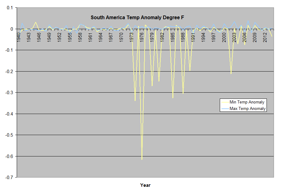


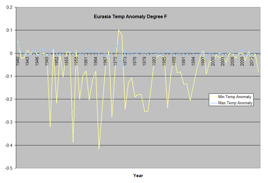


Regional Graphs
Regional annual averaged daily differences.
(Tmin day-1)-(Tmin d-0)=Daily Min Temp Anomaly= MnDiff
(Tmax day-1)-(Tmax d-0)=Daily Max Temp Anomaly= MxDiff
Global Average
US +24.950 to +49.410 Lat: -67 to -124.8 Lon
Tropics -23.433 to +23.433 Lat
Southpole -66.562 to -90 Lat
Southern Hemisphere -23.433 to -66.562 Lat
South America -23.433 to -66.562 Lat: -30 to +180 Lon
Northpole +66.562 to +90 Lat
Northern Hemisphere +23.433 to +66.562 Lat
Eurasia +24.950 to +49.410 Lat: -08 to +180 Lon
Australia -23.433 to -66.562 Lat: -100 to -180 Lon
Africa -23.433 to -66.562 Lat: -100 to -30 Lon
Serious question for the Antarctica experts – if climate sensitivity to carbon dioxide is greater than zero, then how is this possible?:
What are the possible explanations, particularly given very little, if any, water vapor interference?
A serious question I’d like to see answered as well. The greenhouse effect due to increased CO2 concentration should show up as a direct effect with no feedback above deserts. The absolute best place to look for a direct effect is in the temperature cycling between daytime and nighttime temperatures in mid-Sahara, or the Namib, or (as you say) Antarctica. The direct effect expected from CO2 would be a narrowing of the range from daytime high to nighttime low, produced by little to no interference with SW solar warming but an inhibition of nighttime cooling. It would take a decade or two of patient work (since unfortunately no warmist will accept UAH as a proxy for surface temperature because if they did, it would be clear evidence of nonphysical bias in the surface temperature record as the two do not agree) but simple thermometers on an array of carefully sited, mid-desert stations, with care taken to correct for locally measured ambient humidity and so on — should allow the direct no-feedback effect to be directly measured over time to a high resolution.
rgb
The reason there has been no measurable rise in global T from rising CO2 is because the effect is not linear. This chart shows it clearly:
Almost all the global warming from CO2 took place within the first few dozen ppm. At the current ≈400 ppm, any warming from CO2 is simply too tiny to measure.
In fact, if CO2 increased by 20%, 30%, 40%, or more from current levels, any resulting warming would still be too small to measure. Just look at the temperature axis, and extrapolate out to 500 ppm, 600 ppm, etc. Any warming from even a big rise in CO2 would only be a minuscule fraction of a degree. CO2 would still remain a tiny trace gas.
AGW is a baseless scare. I think AGW exists. But even if CO2 doubled (very unlikely), it is a complete non-problem. It is only being used to scare the population into agreeing to ‘carbon’ taxes — which would be a really huge problem.
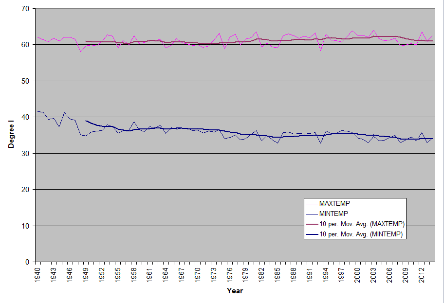
I can provide you all the stations north and south of 66.562 lat back to the 40’s, number of stations, where the stations are located (antarctic has a pretty poor history), north pole is mostly coastal, and there aren’t many in the various deserts, but I can and will create you the reports you want, most of which I’ve already done in one fashion or another, and they don’t show any sign of Co2. They do show regional swings due to the jet stream (where appropriate), @N41,W81 we get both tropical and Canadian air, with a 10-12F swing in temps.
dbstealey September 16, 2015 at 10:27 am
I had factored the Beer-Lambert Law neutering effect into the thought processes behind my question, and there should be some CO2 effect, but there clearly isn’t. In the absence of other explanations, your graph may be wrong and everything should be shifted leftwards such that the doubling effect starts at lower ppms CO2 or, alternatively, any CO2 warming is so low that the effect cannot climb out of the noise (if error bars were to be included on the UAH South Polar graph). If it’s the former, then that should also apply globally and the Antarctic empirical data should be a guide for our modelers (a climate sensitivity of zero, or close to zero might allow for more accuracy). Funnily enough, it was thinking about your graph that also got me thinking about asking this question. I was just waiting for an Antarctica thread to pick my spot.
Otherwise – Ozone ? Antarctic high altitude (CO2 cooling effect) ? Do way below freezing temperatures affect radiation effects/absorption in some way ?
…an interesting question. We should have such stations available in the data set. Nevada may have such records away from major cities.
However clearly the troposphere record precludes CO2 as being responsible for whatever warming actually exists at the surface. CAGW theory demands a greater rate of warming in the troposphere.
“The absolute best place to look for a direct effect is in the temperature cycling between daytime and nighttime temperatures in mid-Sahara, or the Namib, or (as you say) Antarctica …”.
===============================
Great idea but how could you ensure that the data collected were fiddle-free?
That’s the real problem.
The diurnal range at several well-tended stations in the Sahel was examined informally, as I recall, back in the 1990’s by various West African meteorologists. There was no consistent narrowing of the diurnal range, apart from what would be an UHI effect at some larger towns. Clear-cut evidence of any measurable CO2 effect upon surface temperatures remains elusive, despite much academic speculation about never-demonstrated “feedbacks” in the climate system.
Check out Steve Goddard on Parker Arizona
This is a chart of the annual average of day to day surface station change in min temp for N37-49,W104-120 the US Southwest deserts.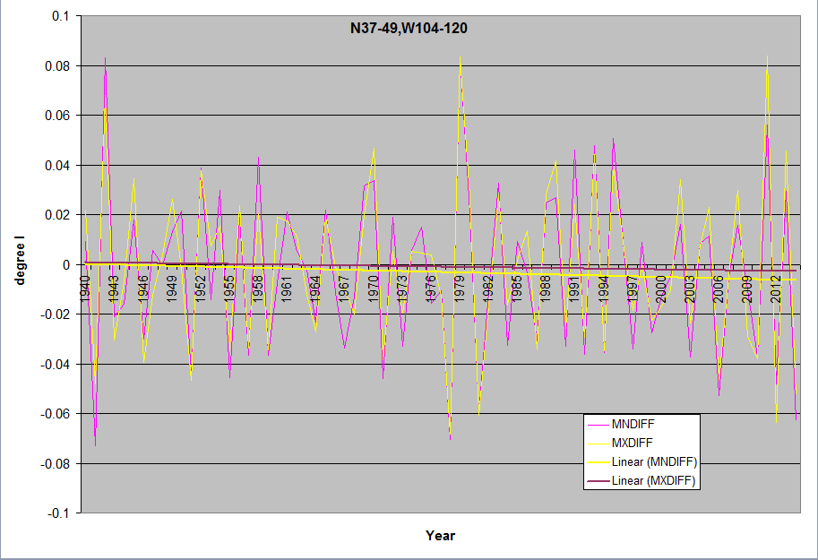
(Tmin day-1)-(Tmin d-0)=Daily Min Temp Anomaly= MnDiff = Difference
For charts with MxDiff it is equal = (Tmax day-1)-(Tmax d-0)=Daily Max Temp Anomaly= MxDiff
MnDiff is also the same as
(Tmax day-1) – (Tmin day-1) = Rising
(Tmax day-1) – (Tmin day-0) = Falling
Rising-Falling = MnDiff
Average daily rising temps
(Tmax day-1) – (Tmin day-1) = Rising
(Tmax day-1) – (Tmin day-0) = Falling
rgbatduke:
I think the issues are covered by Idso’s eight ‘natural experiments’ especially his experiments numbered 2.1 and 2.2.
My link goes to the entire paper that was published in Climate Research (9 April 1998). Its abstract says
emphasis added by me: RSC
The suggested “much more work” has not been undertaken and I failed in my attempts to obtain funding for some of it to be conducted.
Richard
Sorry, I’m not following that – care to expand please?
Seems like Lewis is just sniping. Due to the minimal contributions from water vapor, Antarctica should be the one place that highlight the impacts of CO2. Your graph is just more evidence of low climate sensitivity to CO2, if there’s any at all.
Yes exactly. I was hoping that my question might attract well reasoned answers, as these observations are capable of blowing up the AGW conjecture completely.
philincalifornia,
Here is another T/CO2 chart. It looks very much like the one I posted above:
http://c3headlines.typepad.com/.a/6a010536b58035970c0115707ce438970b-pi
Yeah DB, my point wasn’t that the chart is wrong in principle, but there may be something wrong with the quantitation. For example if, in reality, the x-axis data was actually over to the left a bit, then out at between say 320 and 400 ppm CO2, the effect would be even more minuscule – and a minuscule effect would beget a minuscule temperature increase, as is observed.
This is a good experiment of nature – very little to zero water vapor, a vast, vast expanse of land and ice (missing 5 degrees at the south pole duly noted), and no measurable warming.
Lewis P Buckingham
But the “missing area” (the area not surveyed between 82.5 north (or south) latitude) and the poles is only 2.2 Mkm^2.
Area of the earth = 510 Mkm^2, so that little bit not surveyed by the satellites means … What? (In your opinion.)
(510 – 2x 2.2 Mkm^2) /510 = 99.13 IS covered very adequately; and much more accurately than by tampered land-based weathered boxes next to buildings and asphalt pavement and jet engine exhausts.
Correct me if wrong, as I don’t have the data, but hasn’t the South Pole station shown little or no warming since continuous record-keeping began there? Yet with such low H2O in the air there, that is precisely where CO2 should have the greatest warming effect.
Lewis P Buckingham
???
The last degrees of the poles are not covered by the satellite orbit BECAUSE the satellite rotate from pole-to-pole, but their orbit is not exactly over either pole: They “fly” south from the north pole towards the south pole as the earth’s surface appears to rotate under them from west to east. Thus, since they don’t fly exactly over the pole, that little area around the pole is covered differently than the rest of the earth, and so is not scanned the same and is not included in the original mapped data. The sensors work just fine, but they are not passing over the final degrees of the arctic surface like they do over the rest of the planet.
I should have said greatest direct effect from CO2, since there would be no feedback from increased water vapor.
High summer (January) temperature at the South Pole is −25.9° C. In mid-winter the average temperature is around −58° C.
Although, back radiation from IR, it would seem to me have to come from up welling IR from the surface, and the Arctic and Antarctic because of how cold they are will have the lowest up welling IR from the surface.
“Considering that UAH does not measure north of 85 degrees latitude, nor south of 85 degrees, I’d say your graphic is worthless …”.
=====================================
The surface station anomaly since records began similarly shows no significant long-term trend:
http://www.climate4you.com/images/70-90N%20MonthlyAnomaly%20Since1920.gif
Regional annual averaged daily differences.

(Tmin day-1)-(Tmin d-0)=Daily Min Temp Anomaly= MnDiff
(Tmax day-1)-(Tmax d-0)=Daily Max Temp Anomaly= MxDiff
Southpole -66.562 to -90 Lat
Northpole +66.562 to +90 Lat
These graphs are the day to day average of the individual stations averaged, so there’s no infilling or homogenizing for area that is not measured. What you might expect to see is the difference between min and max or min alone as it’s actually the difference between daily warming and the following nights cooling.
Sorry wrong Graph
Southpole -66.562 to -90 Lat
[What’s the source for that long-term graph of Antarctic temperature anomalies? .mod]
Oops, I linked to the wrong graph:
http://www.climate4you.com/images/70-90S%20MonthlyAnomaly%20Since1957.gif
Lewis P Buckingham
September 16, 2015 at 1:17 pm
RACook. says: “and much more accurately than by tampered land-based weathered boxes ”
…
Nope
…
Satellite MSU’s don’t measure surface temperatures.
===========================================
What does that have to do with RA Cook’s statement? He is asserting that the satellites measurement of the troposphere is more accurate then the surface stations measurement of the surface, and he is correct.
It is also true that CAGW IPCC physics do not allow the surface to warmer faster then the troposphere, which are actually in a slight cooling trend, showing 1998 to be BY FAR the warmest year.
Found this from 2012 on South Pole temperature trend:
http://www.sciencedirect.com/science/article/pii/S0169809512002256
Fifty-year Amundsen–Scott South Pole station surface climatology
Lazzara, et al
“The analysis found slight decreases in the temperature and pressure over the 1957–2010 time period that are not statistically significant. The wind speed, however, does show a significant downward trend of 0.28 m s− 1 decade− 1 over the same period.”
Don’t know how “adjusted” the observations have been.
Gloria Swansong
Ooopsie. And here have been told all along that the ever-greater Antarctic sea ice areas that have been increasing since 1992 have been CAUSED BY the greater Antarctic winds blowing new sea away from the continent land areas!
Lady Gaiagaia,
You are correct
Here is my graph of the month by month winter temperature from the Southpole according to the British Antarctic Survey, and averaged before and after the 1976 regime shift. Like Lazzara study, it shows a slight but insignificant cooling.
http://landscapesandcycles.net/image/73386672_scaled_393x294.png
How can that be, if the hypothesis of man-made global warming has any validity at all?
Over the South Pole, a presumed increase in CO2 since 1915 of almost 100 ppm, with very low H2O in the air, should show at least some warming, with nearly no feedback.
Lewis P Buckingham says:
Satellite MSU’s don’t measure surface temperatures.
Neither do surface stations.
Satellite data is certainly the most accurate global temperature trend data, and the flat temperature trend is corroborated by thousands of radiosonde balloon measurements.
I don’t think skeptics have the same mind-set as the climate alarmist crowd. Speaking for myself, if the global temperature trend was accelerating upward in step with rising CO2 as predicted, I would change my mind.
If the trend and the corellation was decisive enough, and if it lasted for long enough, I would begin to accept that human CO2 emissions were the primary cause of the global warming. Because knowledge is what’s important, not the politics that fuels the AGW debate.
But that hasn’t happened; global warming certainly hasn’t accelerated. In fact, global warming stopped rising a long time ago. The predictions of accelerating warming were wrong. All of them.
Per the Scientific Method, honest scientists should now go back, and try to figure out why their CO2=AGW conjecture has been such a spectacular failure. Skeptical scientists would be happy to assist them in that investigation.
But rather than admit their conjecture has been falsified by Planet Earth, most alarmists refuse to admit those predictions were wrong. How can good science be conducted with that attitude? The answer is: it can’t. Basic honesty is required. That’s what is missing.
Too much money, power, prestige, politics, religious belief, and the fear of being seen to climbdown has poisoned the well. The Real World is showing that the climate alarmists were wrong. But they cannot admit it. They just can’t.
RA,
Yup. Real science hits CAGW with a double whammy!
Lewis,
DB is right for a number of reasons. One is that the supposed sea surface temperatures are not in fact measured at the surface. They used to come from buckets hauled up from various depths, and now come from not well distributed, subsurface floats. The land temperatures are alleged to come from a standard elevation above local level, but often don’t.
But other problems with the so-called “surface data” are even more serious, such as that they are total fabrications.
PS:
RA,
Would be interesting to see actual wind data from the periphery of Antarctica. I’d be surprised if katabatic winds have actually increased in our supposedly warming world, or not.
Gloria Swansong
I have never seen any historical data for antarctic off-coast winds, and have never been given (nor linked to any) trend data showing why (or by how much) any such winds have changed during the many years of antarctic sea ice increase, nor across all of the distances from the coast required to “blow” sea ice away from the coastline. Only hand-waving claims, with no evidence.
RA,
IMO the data are there, but not popularized because they do not serve the interests of the Collective:
http://nsidc.org/data/docs/daac/nsidc0190_surface_obs.gd.html
Lewis P Buckingham:
Your several misleading posts in this thread crescendo with this gem
I admit to a failure:
I tried to discover a way for you to be more wrong than you are in the post I have quoted, but I have failed in the attempt.
So I write to correct the errors in your post.
Surface stations don’t measure surface temperature: they measure air temperature a few feet above the surface. Since you say you are not aware of this I provide you with this link so you will have no excuse for posting such silly nonsense again.
And I don’t understand how dbstealey’s correct point can remind you of a proxy study of “global temperatures for the past 4 billion years”: the present discussion is of attempted direct measurements which have only been made over recent decades.
Of course the microwave sounding units mounted on satellites do indicate temperature because they measure a brightness that indicates temperature. Similarly, mercury-in-glass thermometers also indicate temperature because they measure differential expansions of glass and mercury which indicate temperature. Unless, of course, you want to claim that mercury-in-glass thermometers don’t measure temperature?
And you have provided no laughs so there is nothing of any kind which you have provided that deserves thanks. However, your misleading posts merit disdain so I offer it.
Richard
Phil, it may be that Antarctic inversions cause the CO2 radiating level to be the same or even warmer than the surface, causing an anti-greenhouse effect. If inversions cover half of Antarctica, the net CO2 effect would be nullified. My SWAG.
From the “many a true word is spoken in jest” department, a couple of years ago, on this subject, I speculated that perhaps the issue was that CO2 is upside down in the Southern Hemisphere.
If you’re correct, I may have been closer than I thought !!
richardscourtney is correct about Bucky’s misleading comments. Mr. Buckingham started posting here a couple of years ago, and his comments have become increasingly bizarre. He looks to be fairly new to this subject, and he has clearly arrived at his conclusions without having enough information to make those conclusions.
Now all Buckingham does is look for confirmation bias factoids like his MSU comment, while he constantly denigrates and insults those whose facts and evidence destroy his arguments. The misinformation he posts, and his obvious ignorance that surface stations do not measure surface temperatures, shows that he’s just here to argue, not to learn.
Mr. Courtney made a perfect analogy: that satellites do not directly measure temperature — but neither do thermometers, which simply measure the expansion of a fluid. But we rely on both, and accept both as being accurate when properly calibrated.
Satellites record the most accurate global temperature data, and they cover the planet better — much better — than any other system. That is agreed by all sides of the debate (with a few exceptions, but those exceptions never compare satellite data with GISS’s massaged fabrications, for instance). Even the IPCC admits that temperatures have “paused” for many years.
The government would not pay out hundreds of millions of dollars to launch and maintain satellites if their data was not accurate. Satellite data is corroborated by many thousands of radiosonde balloon measurements, taken from all over the planet year round. The two systems are in agreement, unlike GISS and many others.
Further, exact temperature measurements, while done best by satellites, are not as important as measuring the temperature trend. The trend shows us that global warming stopped many years ago, because the trend is flat to declining (depending on the time frame). That fact decisively falsifies the ‘dangerous AGW’ argument — the basic contention of the entire alarmist crowd. They were wrong in their predictions: rising CO2 has not caused the predicted runaway global warming — or any meaningful global warming, for that matter.
In any other of the hard sciences, that would be the end of it. The scientists and organizations that made those falsified predictions would have to go back and try to find out why their conjecture was so wrong.
But in ‘climate science’, that doesn’t happen. The Scientific Method is ignored. The “dangerous man-made global warming” hoax is now 100% political on the side of the alarmist crowd, and now they have entered the denial stage: they are lying outright when they claim that the ‘pause’ never happened.
Their few enablers here are head-nodding in agreement with that disingenuous prevarication, because some folks simply cannot ever admit that they were wrong — no matter what the data shows.
Richard Courtney,
Bucky says: you have the problem of the fact that satellites don’t take measurements FROM THE SURFACE, whereas thermometers do.
What we have here is a thoroughly confused individual who still does not understand that surface stations do not measure surface temperatures. They measure air temperatures, as satellites do. The air circulates. Each measuring device does it slightly differently. Radiosonde balloons also use thermometer equivalents to measure air temperature.
Bucky is just tap-dancing now, trying to re-frame his argument, to claim that surface station thermometers measure the ground. They don’t. They measure air temperatures like all the other land and satellite systems.
So as usual, Bucky is wrong. No need to explain more to him, he wouldn’t get it anyway.
Bucky sez:
…you can continue to pick the dataset that supports your positions, but alas, that is just another case of cherry picking on your part.
LOLOL!! That comment is pure psychological projection, as Bucky shamelessly cherry-picks <a href=http://www.woodfortrees.org/plot/rss/from:2011/plot/rss/from:2011/trend a few short years out of the trend, beginning in 2011, when he knows temps were at the low end of the 2011 – 2015 range.
Could Bucky be any more hypocritical, and disingenuous?
Global warming stopped in the late ’90’s:
http://www.woodfortrees.org/plot/rss/from:1997/plot/rss/from:1997.9/trend
Even the IPCC admits to that fact.
So go argue with them, Bunky. You’re in over your head here.
dbstealey:
You advise me
Thankyou. I will accept your advice because it is obviously true. For example I gave a link that explains Stevenson Screens saying to him
and he has replied
Clearly, either Lewis P Buckingham cannot read or he chooses to not read corrections to his silly mistakes.
And I note that each and every statement he has made in this thread is a silly mistake.
Richard
Lewis,
So you agree that Arctic ice extent measured is worthless too? We don’t have to worry about sea ice because it’s not measured from the surface.
Surface temperatures are not recorded 85N+ in GISS or HADRCUT3/4 so how does that make satellite worthless compared?
The coverage of up to 85S is by far more than GISS or HADCRUT and shows Antarctica slightly cooling from 1979.
http://i772.photobucket.com/albums/yy8/SciMattG/UAH_AntarcticOceanTemps_zpsyk6tsbmm.png
The purpose is to observe whether the planet gains or loses energy over a period of time and the satellite covers far more of the atmosphere than isolated pockets on the surface will ever do. The surface being 4 ft off the ground, not the ground temperature.
How does RSS look now from 1979?
http://i772.photobucket.com/albums/yy8/SciMattG/RSS%20Global_v1997-01removal_zpszk83g0xi.png
You do realize to cause a linear trend to become flat from 1979 requires the same amount of cooling as warming in the first place. When it has reached this point global temperatures must have already cooled equally for a significant time, almost the same as the warming in the first place. Hence, you are denying a significant decrease in the rate of temperature change.
Lady G says:
Lewis, DB is right for a number of reasons…
Lady G, Lewis lives in his own alternate universe. He is wrong when he says that satellites don’t take measurements FROM THE SURFACE, whereas thermometers do.
We have repeatedly tried to explain to him that none of the systems discussed are measuring anything other than air temperatures. But he keeps digging his hole deeper.
So I give up. Bucky is convinced that thermometers measure the temperature of the earth’s surface, and nothing can penetrate his Belief. Certainly not logic, or clear, rational explanations. Buckingham probably saw the words “Surface Stations”, and decided that they mean what he wants them to mean: thermometers measure the temperature of the ground.
For new readers who may wonder, ‘surface stations’ measure air temperatures, from about six feet above the surface. They are located on the surface instead of in balloons or on satellites, that’s all.
Mr. Bucky is also incorrect here:
Stealey says: “The trend shows us that global warming stopped many years ago”
RSS shows something very different..
The longer the observed trend, the more information it contains, and thus the more accurate it is. Lewis B makes the same deliberate error that the great John Daly wrote about here.
Ben Santer tried to pull a fast one, by posting the chart below in the journal Nature, deviously attempting to show “human influence” in global warming:
http://www.john-daly.com/stats1.gif
But Santer deliberately removed important data. Here is the full chart:
http://www.john-daly.com/stats2.gif
We see that Santer cut off years of data, and began his chart at a time that appeared to show steadily rising temperatures. That is exactly what Lewis B did with his truncated RSS chart.
As John Daly wrote:
When the full available time period of radiosonde data is shown we see that the warming indicated in Santer’s version is just a product of the dates chosen.
L. Buckingham did exactly the same thing; he chose dates that appear to show global warming, just like Santer did.
Dr. Santer was refuted by both American and German scientists. His lack of probity was publicized when …’Nature’ published two rebuttals from other climate scientists, exposing the faulty science employed by Santer et al. (Vol.384, 12 Dec 1996).
The Latin proverb:
Falsus in uno, falsus in omnibus applies to both Santer and Buckingham.
The proof is in the Nature rebuttal, and in the highly selective, cherry-picked chart fabricated by Lewis Buckingham.
Here, the difference between air and ground temps
https://stevengoddard.wordpress.com/2015/09/15/26-increase-in-arctic-sea-ice-over-the-last-three-years/
So, what was your problem, again?
Once again Jim I am in agreement with all the points you are making.
Jim ,I think all of these factors going forward will lead to global cooling not warming.
I think Milankovich Cycles, the Initial State of the Climate or Mean State of the Climate , State of Earth’s Magnetic Field set the background for long run climate change and how effective given solar variability will be when it changes when combined with those items. Nevertheless I think solar variability within itself will always be able to exert some kind of an influence on the climate regardless if , and that is my hurdle IF the solar variability is great enough in magnitude and duration of time. Sometimes solar variability acting in concert with factors setting the long term climatic trend while at other times acting in opposition.
THE CRITERIA
Solar Flux avg. sub 90
Solar Wind avg. sub 350 km/sec
AP index avg. sub 5.0
Cosmic ray counts north of 6500 counts per minute
Total Solar Irradiance off .15% or more
EUV light average 0-105 nm sub 100 units (or off 100% or more) and longer UV light emissions around 300 nm off by several percent.
IMF around 4.0 nt or lower.
The above solar parameter averages following several years of sub solar activity in general which commenced in year 2005. The key is duration of time because although sunspot activity can diminish it takes a much longer time for coronal holes to dissipate which can keep the solar wind elevated which was the case during the recent solar lull of 2008-2010 ,which in turn keep solar climatic effects more at bay. Duration of time therefore being key.
If , these average solar parameters are the rule going forward for the remainder of this decade expect global average temperatures to fall by -.5C, with the largest global temperature declines occurring over the high latitudes of N.H. land areas.
The decline in temperatures should begin to start to take place within six months after the ending of the maximum of solar cycle 24,if sub- solar conditions have been in place for 10 years + which we have now had. Again the solar wind will be needed to get to an average of below 350km/sec. which takes time because not only do the sunspots have to dissipate but also the coronal holes. In other words a long period of very low sunspots will be need to accomplish this. It will be a gradual wind down..
Secondary Effects With Prolonged Minimum Solar Activity. A Brief Overview. Even if one or two should turn out to be true it would be enough to accomplish the solar /climatic connection.
A Greater Meridional Atmospheric Circulation- due to less UV Light Lower Ozone in Lower Stratosphere.
Increase In Low Clouds- due to an increase in Galactic Cosmic Rays.
Greater Snow-Ice Cover- associated with a Meridional Atmospheric Circulation/an Increase In Clouds.
Greater Snow-Ice Cover probably resulting over time to a more Zonal Atmospheric Circulation. This Circulation increasing the Aridity over the Ice Sheets eventually. Dust probably increasing into the atmosphere over time.
Increase in Volcanic Activity – Since 1600 AD, data shows 85 % approximately of all major Volcanic eruptions have been associated with Prolonged Solar Minimum Conditions. Data from the Space and Science Center headed by Dr. Casey.
Volcanic Activity -acting as a cooling agent for the climate,(SO2) and enhancing Aerosols possibly aiding in greater Cloud formation.
Decrease In Ocean Heat Content/Sea Surface Temperature -due to a decline in Visible Light and Near UV light.
This in turn should diminish the Greenhouse Gas Effect over time, while promoting a slow drying out of the atmosphere over time. This may be part of the reason why Aridity is very common with glacial periods.
In addition sea surface temperature distribution changes should come about ,which probably results in different oceanic current patterns.
http://wattsupwiththat.com/2015/09/01/the-arctic-iris-effect-dansgaard-oeschger-events-and-climate-model-shortcomings-lesson-from-climate-past-part-1/
The above accounts for abrupt climatic changes within a glacial or inter- glacial period.
SalvatoreDel Prete says “all of these factors going forward will lead to global cooling not warming”…
“I think solar variability within itself will always be able to exert some kind of an influence on the climate regardless”
I agree. In part 3 I will discuss how I see the contributions from solar variability.
I just bought a new, bigger snow plow truck and new snow plow even though the jeep and plow still works. Preparing for nasty weather in winter in the Northeast in the future…. 🙁
The Cretaceous has always been a problem for GCMs. Even when Cretaceous CO2 was thought to be around 2000 ppm or more, the models needed ECS of at least six degrees C to reproduce the great warmth of its climate and how equable it was from equator to poles, as shown by all proxies.
This failure may be due to the models’ ignoring the effect of clouds or lack thereof.
Please include a citation to the source of all text, and, especially, graphics used in articles and comments. If, of course, the graphic is of the author’s own creation, then reference the data source.
I find that when discussing “climate change” with friends, they just won’t accept WUWT as a reliable source. (Sorry, Anthony – you have a reputation. But living as you and I do, within a short distance of Sillywood, I guess any publicity is good publicity.)
Also, when I was in engineering school, failure to reference a source would result in mark-downs. Since we aspire to science here, let’s try to follow the discipline.
Except for what the graph of the Cenozoic cooling that I thought was a generic illustration, there are links to all the other the texts and graph.
Continental disposition due to plate tectonics and corresponding oceanic currents disposition might explain why this Quaternary Ice Age is much colder than the previous one, but it does not explain why there is a Quaternary Ice Age in the first place, as ice ages are a feature of the Earth that take place every 150 million years. In about 10 million years our ice age should peter out, although Homo sapiens is not expected to last that long. As we are unlucky to be a species born in the 1% of the coldest times of Earth, we are all oh so lucky to have been born during the 10% of the warmest times of this ice age, and we are all going to die within that period also, so we shouldn’t be very concerned about the climate as individuals.
Primary CO2 production comes from the mantle through volcanic activity. As the Earth cools down volcanic activity is inexorably reducing despite important but occasional outbursts from volcanic traps. Thus CO2 levels, that have reached almost plant starvation levels prior to mankind release of fossil carbon, are expected to continue reducing in the future, reducing atmospheric density and ultimately oxygen levels, since oxygen proceeds mainly from CO2. Lower oxygen and atmospheric density has important biological consequences. Already we have nothing bigger than a condor capable of flying in our atmosphere, while Argentavis, with over 3 meters of wingspan, flew prior to current ice age and Quetzalcoatlus, with a wingspan of 11 meters flew in the CO2 rich Cretaceous. Also animal size has been going down with time, and very large mammals like Indricotherium, Deinotherium and Mammoth do no longer exist. The future belongs to mice.
The biggest animals to ever roam the earth are the Blue Whales and whales began evolving along with DIatoms and the ACC
Whales play a different league. Their metabolism is much lower per unit of mass than any land mammal. When beached they suffocate shortly due to their own weight. But they are proof that there are always animals that grow to maximum size allowed by physical constraints when food is not a problem. Today’s physical constrains on land and air are much lower than previously. Two meter wingspan dragonflies are simply impossible, when they were not previously.
I disagree. The diatom take-over is controversial and placed between the Cretaceous and the Cenozoic. Nobody really knows when the ACC formed. It is all speculation as oceanic currents do not fossilize well. Baleen whale size evolution is tied to krill abundance. Krill abundance is tied to ocean productivity. Ocean productivity is higher the drier (and colder) conditions are on land so dust production is increased and fertilizes the oceans. Cetaceans shoot their maximal size starting about 15-20 million years ago, when the planet got colder and Antarctica started to have a permanent ice sheet. These are facts.
An old reference on the evolution of modern whale types in the Oligocene and Miocene, but still IMO useful. More recent advances in knowledge of whale evolution are earlier, during the Paleocene and Eocene Epochs.
http://www.sciencedirect.com/science/article/pii/0031018280900243
Whale evolution and Oligocene southern ocean environments
Fordyce
Abstract
Many odontocetes [modern toothed whales, Early Oligocene (35 Ma) — Recent] utilise high-frequency echolocation to facilitate predation, while mysticetes (baleen whales, Early Oligocene—Recent) possess a filter-feeding system which allows cropping of plankton. These adaptations are reflected in the unique skull structure of each group. Skulls of archaeocetes [primitive toothed whales, the ancestors of odontocetes and mysticetes, Middle Eocene—Late Oligocene (45 to 25 Ma)] indicate that they possessed neither baleen nor the capacity for echolocation. Studies on Northern Hemisphere Cetacea (whales and dolphins) have suggested a paucity of Oligocene Cetacea but also have stressed that the Oligocene was an important time in cetacean evolution. The observation of some authors that cetacean diversity declined in the Oligocene has been difficult to reconcile with the origins then of odontocetes and mysticetes. Hypotheses have stressed that the “decline” reflects decreased oceanic thermal gradients, upwelling, plankton diversity and thus fewer cetacean niches. The Austral Oligocene fauna allows alternative explanations. The earliest known mysticetes and odontocetes are New Zealand Early Oligocene forms. Their appearance probably was triggered by the initiation of the psychrosphere and concomitant Austral increases in upwelling and productivity. Austral cetacean radiations in the Middle Oligocene are attributable to the influence of the Circum-Antarctic Current on regional productivity and the creation of more new niches. The decline of archaeocetes, further radiations of odontocetes and mysticetes, and the development of a cosmopolitan cetacean fauna in the Late Oligocene (25 Ma) foreshadowed the radiation of modern cetacean stocks with the establishment of major “modern” ocean patterns in the Miocene (22-5 Ma).
Javier to say “Nobody really knows when the ACC formed” is a tad inaccurate. There is indeed debate on the exact timing and the strength but it is pretty clear that it was close to full strength by the time Antarctic glaciation began. And the current does leave fossil. Organisms restricted to the Pacific before the Drakes Passage gateway opened and then suddenly show up in the Atlantic suggesting the time when the ACC was beginning. Similar evidence for the Tasmanian Gateway.
From the Bijl paper I linked to in the essay, “Dinoflagellate biogeography and sea surface temperature
paleothermometry reveal that the earliest throughflow of a westbound Antarctic Counter Current began ∼49–50 Ma through a southern opening of the Tasmanian Gateway. This early opening occurs in conjunction with the simultaneous onset of regional surface water and continental cooling (2–4 °C), evidenced by biomarker- and pollen-based paleothermometry”
contrary to catastrophic CO2 assertions that rising CO2 will decimate calcium carbonate shell producers, the greatest proliferation of calcium carbonate shell producers occurred during this period with the high temperatures and high concentrations of atmospheric CO2.
=====================
O2 + 2Ca + 2CO2 === 2CaCO3
adding more CO2 on the left will not reduce the amount of CaCO3 (shell) on the right. this is basic chemistry.
The fallacy in “ocean acidification” comes from treating the oceans as acidic. Since acids dissolve CaCO3 , ocean acidification must reduce shell. But of course ocean acidification does not make the oceans acidic, which means adding CO2 will not reduce shell. it will increase the raw materials for building shell.
Thanks, Dr. Steele.
This is a good article. Funny how nature is denying the warmista narrative.
Could be. But IIRC, prior to the KT extinction event mammals were small, terrestrial, and probably not very common. It was only after the disappearance of most terrestrial reptiles 64 million years ago that mammals started to expand in size and diversity. I think many (most?) vertebrate paleontologists might regard the development of diverse marine, mammalian carnivores starting in the Early Eocene as an expansion by mammals into largely empty ecological niches formerly occupied by mosasaurs.
No doubt that vacant niche played a role.
That might explain why toothed whales evolved from seal-like coastal artiodactyls, but the biggest whales are baleen and feed primarily on krill, with some fish.