Guest Post by Willis Eschenbach
Well, either it’s a genetic defect or I’m just a glutton for punishment, but I’m going to delve some more into the ice ages. This is a followup to my previous post, Into and Out Of The Icebox. Let me start by looking at the cycles in the insolation and the cycles in the geological temperature. I’ll use the same temperature proxy dataset used in the discussion by Science of Doom here and here, which is the Huybers ∂18O dataset . For the insolation, I’m using the same Berger dataset that I used in my last post. Figure 1 shows the cycles in the two datasets:
 Figure 1. Periodogram of the Huybers temperature proxy dataset (blue) and the June insolation at 65°N from the Berger geological insolation dataset.
This graph demonstrates extremely clearly what is called the “100,000 year problem”. As you can see, the length of the ice ages has a very strong 100,000 year cycle, with a cycle amplitude greater than 40% of the swing of the data.
But in total contradiction to that, the June insolation at 65°N, which is the insolation that is supposed to cause the interruptions of the ice ages, has virtually no cycle strength in the 100,000 year (100 Kyr) range. The insolation has its greatest cycle strength between 19 and 24 Kya, and a smaller peak at 41 Kyr, but there is almost no power at all in the 100 Kya range.
It is worth noting that both the temperature and the insolation do show power in the ~ 23 Kyr and the ~ 41 Kyr range … but only the temperature has power in the 100 Kyr range.
Now, back in 2006 Gerald Roe wrote a paper called “In Defense of Milankovich”. In that paper, he said that the reason there was little relationship between the Northern Hemisphere insolation and the ice ages was that people were looking at the wrong thing. His point was that when the sun increases, the ice doesn’t immediately disappear. Instead, what changes is the rate of melting of the ice. This is also called the “first difference” of the ice volume. Roe used an earlier version of the same Huybers temperature proxy dataset I’m using to demonstrate his hypothesis, reasoning that the ice volume is a function of the global temperature.
So let’s start by looking at the effect of taking the first differences on the underlying cycles. Figure 2 is the same as Figure 1, except that I’m using first differences instead of using the raw Huybers temperature proxy data.
 Figure 2. Periodogram of the first difference of the Huybers temperature proxy dataset (blue) and the June insolation at 65°N from the Berger geological insolation dataset.
Now, that is an interesting result. As you might imagine, it hasn’t introduced any new frequencies into the mix. However, it has greatly decreased the size of the 100 Kyr cycle, slightly increased the size of the 23 Kyr cycle, and slightly decreased the size of the 41 Kyr cycle.
And what would be the result of those changes? Well, the correlation will indeed be better, as Roe observed … but for the wrong reasons. The correlation will be greater because in the temperature data (blue) the ~ 20 Kyr cycle and 41 Kyr cycles are now about the same size as the 100 Kyr cycle. So those cycles will fit better … but we still have no explanation for the 100 Kyr cycle.
In any case, here’s the match between the June insolation at 65°N and the first difference of the temperature proxy:
 Figure 3. A comparison of the June insolation at 65°N (red) and the first difference of the ∂18O temperature proxy. I am using the negative of the ∂18O data, so that increasing values show increasing temperatures.
Looks good, doesn’t it … but it’s not. Unfortunately, this is merely a wonderful example of the human propensity for seeing patterns. If you look at parts of this, it looks like a perfect match. The problem is, humans are shaped and bred by millions of years of evolution to find visual patterns … and as a result we find patterns even where no such patterns exist. The best example I can give you is that virtually every culture has found constellations in the stars. We identify Orion and Gemini and a host of others … and despite that, the stars contain no such patterns, just a random scatter.
And when we look closely at Figure 3, we can see that in many of the cases, the blue lines are in between the red lines … in all, they seem to be aligned at around 600 Kyr BP and also around the present, but badly out of alignment in between.
In order to keep ourselves from making such mistakes in pattern identification (among other reasons), we’ve invented an entire branch of mathematics called statistics. It allows us to do things like measure just how much of one variable is explained by another variable. The measure of this is called “R^2”. It varies from 0.0 (no relationship) to 1.0 (one variable totally explains the other).
And the R^2 value for the two variables above? How much of the first difference of the temperature variation is explained by the variation in northern insolation?
Well, the R^2 of the two is a mere 0.05 … that is to say, the June insolation at 65°N only explains about 5% of the variations in the first difference in temperature. Color me unimpressed.
Now, it’s possible that there is some lag in the data. To check that, we can run a “cross correlation”. This looks at the correlation, not just at the same time, but at a variety of time lags. Here is the cross correlation of the two variables:
 Figure 4. Cross correlation of insolation and first difference of temperature. Positive lags show temperature changes lagging insolation changes. Blue lines show the level where the p-vaule is 0.05, which must be exceeded to achieve statistical significance.
So … there you have it. The relationship just barely achieves statistical significance. Is it true that looking at the first difference of the temperature improves the correlation? Yes, it is … but for the wrong reason. Taking the first difference of the temperature proxy reduces the amplitude of the 100 Kyr signal and increases the amplitude of the ~20 Kyr signal. Since the ~ 20 Kyr signal is the largest signal in the insolation, as a result the overall correlation increases … but this still doesn’t help us at all with the “100,000 year problem”. Not only that, but at the end of the day, the relationship is so weak as to scarcely achieve statistical significance.
Me, I’d say that Roe certainly didn’t solve the 100,000 year problem … although as always, YMMV …
Best wishes to everyone,
w.
My usual request—if you disagree with someone, please QUOTE THEIR EXACT WORDS THAT YOU DISAGREE WITH. This is the only way for everyone to be clear as to the exact ideas that you are objecting to.
I have a couple of comments relative to the data underlying this thread.
First, the peak in both temperature and insolation at 2kyr is not an artifact of the sampling period except for the issue of aliasing which I question in my second point below. The Nyquist frequency at delta-t of 1 kyr is one period per 2 kyr, so the signal at 2 kyr, assuming no aliasing, resolves just fine; however the periodogram value at the Nyquist rate is utterly dependent on sampling phase, and so the amplitude should have very large error bars associated with it. Back when I was doing seismic processing for oil exploration we generally thought a sampled signal should have at least 5 sample points per cycle, rather than the two available at the Nyquist rate. So that portion of data below 5kyr cycle isn’t worth much.
Second, the isotope data are not “point” values, but rather have a sampling window, dependent on field sampling and laboratory methods, which smears time resolution. What is the nature of the sampling window? Can anyone answer this question without my having to dig through discussion of field technique that may not exist anywhere? Perhaps at the top of some column (ice or ocean sediment) the window is minus 500 years to plus 500 years, but column compaction, which occurs in both ice and sediments, might make the sampling window much wider at 100Kyr or 400kyr. On the other hand a very narrow sampling window may leave the isotope data aliased–i.e. placing short period features in the geological column as artifacts in the periodogram at periods of 2kyr and longer.
Finally, I question the value of correlating insolation against temperature, when the insolation may not impact temperature directly, but has to operate through feedback subject to the complex dynamics of the atmosphere, and so forth. Lack of correlation I don’t see as a definitive test of Milankovitch cycles.
From Don Easterbrook – Aside from the statistical analyses, there are very serious problems with the Milankovitch theory. For example, (1) as John Mercer pointed out decades ago, the synchroniety of glaciations in both hemispheres is ‘’a fly in the Milakovitch soup,’ (2) glaciations typically end very abruptly, not slowly, (3) the Dansgaard-Oeschger events are so abrupt that they could not possibility be caused by Milankovitch changes (this is why the YD is so significant), and (4) since the magnitude of the Younger Dryas changes were from full non-glacial to full glacial temperatures for 1000+ years and back to full non-glacial temperatures (20+ degrees in a century), it is clear that something other than Milankovitch cycles can cause full Pleistocene glaciations. Until we more clearly understand abrupt climate changes that are simultaneous in both hemispheres we will not understand the cause of glaciations and climate changes.
My reply
All the above which is what the data shows lends support to my thoughts that solar variability and the primary and secondary effects associated with this solar variability are a big player in glacial/inter-glacial cycles when taken into consideration with these factors which are , land/ocean arrangements , mean land elevation ,mean magnetic field strength of the earth(magnetic excursions), the mean state of the climate (average global temp), the initial state of the earth’s climate(how close to interglacial-glacial threshold it is) the state of random terrestrial(violent volcanic eruption) /extra terrestrial events (super-nova in vicinity of earth or a random impact) along with Milankovitch Cycles. These factors setting the back ground for a general climatic trend for the earth to move in if solar variability did not exist at all.
What I think happens is those factors keep the climate of the earth moving in a general trend toward either cooling or warming on a very loose cyclic or semi cyclic beat but get consistently interrupted by solar variability and the associated primary and secondary effects with this solar variability which brings about at times counter trends in the climate of the earth within the overall trend , or at other times when all the factors I have mentioned setting the back ground for the climate trend for cooling or warming along with what solar variability has been doing in conjunction with these factors , then drive the climate of the earth gradually into a cooler/warmer trend UNTIL it is near that inter- glacial/glacial threshold or climate intersection that makes any further solar variability no matter how slight at that point to be enough to cascade the climate into an abrupt climatic change. The back ground for the abrupt climatic change being in the making all along but when the threshold glacial/inter-glacial intersection for the climate is reached that is NOT ONLY when the abrupt climatic changes occur but the constant swings in the climate from glacial to inter-glacial over short periods of time can take place .
The climatic back ground factors along with the general trend in solar activity driving the climate gradually toward the climate intersection or threshold of glacial versus interglacial, then once there at the intersection the climate gets wild and abrupt.
The climate is chaotic, random and non linear but in addition is never in the same mean state or initial state which makes given forcing to the climatic system not resulting in a given outcome which is why I think there is a semi cyclic nature to the climate but it is consistently being disrupted with counter- trends at times or abrupt changes at times.
If what I say is not on the correct path then why is it whenever the climate strays from its mean in either a negative or positive direction it is ALWAYS brought back to its mean. Why does the climate never go in the same direction once it heads in that direction?
Why is it that when the ice sheets expand the lower albedo /lower temperature more ice expansion positive feedback does not keep going once it is set into motion? What causes it not only to stop but reverse?
Vice Versa why is it when the Paleocene – Eocene Thermal Maximum came about that the increase CO2/higher temperature positive feedback not only did not keep proceeding but reversed?
I will have a follow up post to this one.
My follow up.
Below I list my low average solar parameters criteria which I think will result in secondary effects being exerted upon the climatic system.
My biggest hurdle I think is not if these low average solar parameters would exert an influence upon the climate but rather will they be reached and if reached for how long a period of time?
I think each of the items I list both primary and secondary effects due to solar variability if reached are more then enough to bring the global temperatures down by at least .5c in the coming years.
Even a .15 % decrease from just solar irradiance alone is going to bring the avg. global temperature down by .2c or so all other things being equal. That is 40% of the .5c drop I think can be attained. Never mind the contribution from everything else that is mentioned.
What I am going to do is look into research on sun like stars to try to get some sort of a gage as to how much possible variation might be inherent with the total solar irradiance of the sun. That said we know EUV light varies by much greater amounts and within the spectrum of total solar irradiance some of it is in anti phase which mask total variability within the spectrum. It makes the total irradiance variation seem less then it is.
I also think the .1% variation that is so acceptable for TSI is on flimsy ground in that measurements for this item are not consistent and the history of measuring this item with instrumentation is just to short to draw these conclusions not to mention I know some sun like stars (which I am going to look into more) have much greater variability of .1%.
I think Milankovich Cycles, the Initial State of the Climate or Mean State of the Climate , State of Earth’s Magnetic Field set the background for long run climate change and how effective given solar variability will be when it changes when combined with those items. Nevertheless I think solar variability within itself will always be able to exert some kind of an influence on the climate regardless if , and that is my hurdle IF the solar variability is great enough in magnitude and duration of time.
THE CRITERIA
Solar Flux avg. sub 90
Solar Wind avg. sub 350 km/sec
AP index avg. sub 5.0
Cosmic ray counts north of 6500 counts per minute
Total Solar Irradiance off .15% or more
EUV light average 0-105 nm sub 100 units (or off 100% or more) and longer UV light emissions around 300 nm off by several percent.
IMF around 4.0 nt or lower.
The above solar parameter averages following several years of sub solar activity in general which commenced in year 2005..
IF , these average solar parameters are the rule going forward for the remainder of this decade expect global average temperatures to fall by -.5C, with the largest global temperature declines occurring over the high latitudes of N.H. land areas.
The decline in temperatures should begin to take place within six months after the ending of the maximum of solar cycle 24.
Secondary effects on temperature as a result of prolonged solar activity I think will be the following:
A meridional atmospheric circulation due to less UV Light lower ozone in Lower Stratosphere.
Increase in low clouds due to an increase in galactic cosmic rays.
Greater snow-ice /cover associated with a meridional atmospheric circulation.
Increase in volcanic activity – Since 1600ad data shows 85 % of al major volcanic eruptions associated with prolonged solar minimum conditions. Space and Science Dr. Casey has the data.
Decrease in ocean heat content/sea surface temp due to a decline in visible light near UV light.
That is my take from the studies I have done over the years correct or not.
Loehle:“… Bering straits,… and ice increases (gradual cooling) but when it gives way it is more sudden and the ice begins to melt rapidly. These processes are threshold events and take a very long lag to get to.”
It just occurred to me that this might be the mechanism for the relaxation oscillator discussed in my 9:46am reply* to fhhaynie above, where I said the glaciation history doesn’t look like a relaxation oscillation because the response is a fast-rise followed by a slow-fall.
But after some reflection I realize this does fit the relaxation model rather well if you simply invert the plot. So I think fyhaynie’s remark was very perceptive.
http://i62.tinypic.com/5cyvdv.jpg
So, instead of a “sudden rise in CO2 ppm” we could interpret the curve as some sudden “loss of equilibrium in system X” followed by a slow return to “equilibrium in system X”, where System X could be the Bering Straights undergoing a dam-building process, which progresses slowly until the dam breaks, causing a relatively rapid loss of equibrium, then followed by a relatively slow return to equibrium, as the dam is rebuilt. (Actually, it’s ‘quasi-fractal’; you can see a series of smaller ‘relaxation’ events embedded in the larger events, suggesting minor breaches while the dam was rebuilding.)
The rate of growth curve in X does resemble the time plot of a capacitor recharging with a time constant of RC:
http://hyperphysics.phy-astr.gsu.edu/hbase/electric/imgele/capchg.gif
So this (or similar oscillating systems) might be the proper reference frame to interpret this kind of temperature history.
—————————————
* Willis, in the quoted reference, I inadvertently left out a closing angle bracket in the html “slow rising-fast falling</i?” This improperly italicized everything. Could you possibly replace the ‘?’ with the proper angle bracket? Thanks!
There is something to this. Or the well known variant, a one shot / ___ 123 chip and ancillary components.
Besides a Bering dam there may also be something with how ice tends to pile / get compressed up along the north coasts of Greenland and the Canadian Archipelago.
Willis Eschenbach, just out of curiosity, I decided to take this commenter at Climate Etc. up on his suggestion and convey his message to you. I am just as interested as he, as the material you present here is new to me and although it doesn’t completely surprise me (as I have, for some time, thought of the apisidal precession as the switch in Milankovich) but nevertheless seems to redefine Milankovich. I’d greatly appreciate your response to this:
http://judithcurry.com/2015/01/24/week-in-review-40/#comment-668423
Thanks, ordvic. I’m afraid I’ll have to pass on this one. I don’t do third-party discussions, because things always get lost in the translation. If he wants to come over here and ask me himself, I’m more than happy to discuss it with him.
Normally I’d answer him there. However, his comment starts off by saying “Regarding Willis on WUWT (where I refuse to comment).”. If that’s his attitude, I’m not interested. I heartily invite him to come and raise his objections here, and we can discuss it.
My best to you, and my invitation to him is sincere … whether he is sincere is another question.
w.
Well perhaps you could answer my quandary instead. I noticed quite some time ago that the 100,000 temp cycle didn’t match the eccentricty cycle as that seemed to take place inbetween the two peaks of interglacial. Then I found out through Kern et al that the apisidal precession caused by orbital tilt has a 3 million mile eccentricity itself. He thinks it is the reason for the current situation with a melting arctic and expanding antarctic. In the absence of the eccentricity cycle the temperature goes up but then it goes down again. The apisidal precession seems to explain this:

During the Eemian this took 22,000 years to complete the cycle. The glacial period started about 110,000 yb and ended about 12,000 yb. So if that is correct we would have another 10,000 years to complete the cycle. Currently Kern has the summer apisidal at about Jan 7 with a day changing every 58 years. That seems to be in line with being just past a half a cycle. I may be all mixed up here as I’m not a scientist. So my question is does the precession cause the temperature to go down as it slowly shifts to the NH?
I seem to have lost the jpg. I’ll try again
http://theinconvenientskeptic.com/wp-content/uploads/2012/01/Chap_6-Illustration_45.png
easy peasy
Can you discuss this chart
http://lh4.ggpht.com/_4ruQ7t4zrFA/TDL7RSCEgZI/AAAAAAAAEGE/0HeA3XYGVmM/s1600/milankovitch-roe-fig2.JPG
Steven Mosher January 25, 2015 at 7:52 pm
Discuss that wiith you? No way. You think that you can block me on Facebook because you didn’t like my ideas, and then talk nice to me here? Not happening, Mosh. Sorry, but it’s all or nothing. You want to block me there, you can’t talk to me here.
w.
Why does your periodogram not register the ~100kyr modulation?
Ummm … because there isn’t one? The periodogram shows the underlying frequencies. Do the Fourier transform yourself if you don’t believe me.
w.
Yup the range is modulated on a ~100kyr cycle:
http://snag.gy/eGc6Y.jpg
Willis,
I tried it myself, which leads me to some questions that should have occurred to me when I looked at your figure, except that it has been a while since I’ve Fourier transforms. The transform gives results at equal frequency intervals, so when converted to period the points are crowded together at short periods and spread out at long periods, even when plotted on a log scale. But your graph does the opposite. It looks like you might have points at equal cycle lengths. How did you do that? Can you provide a reference?
My other question might not be relevant depending on the answer to the above: How long a window did you use?
Mike M. January 25, 2015 at 4:17 pm
I use a variation of Fourier analysis that I discovered myself, and which I was later informed by Tamino is actually called the “Date-Compensated Discrete Fourier Transform”, or DCDFT (Ferraz-Mello, S. 1981, Astron. J., 86, 619). It is tolerant of missing data, and gives (as you noted) results at equal cycle lengths.
I pre-filtered the data using a Hanning window which has the same length as the data.
w.
Thanks, Willis. I will look at the paper and give it a try. It would seem to have some definite advantages compared to a traditional FT power spectrum.
See http://wattsupwiththat.com/2015/01/24/the-icebox-heats-up/#comment-1843647
Ulrich, see johanus’s comment linked to above.
w.
That’s the wrong pole. Those kind of processes are behind the DO events in the Arctic. And it’s just talking around my point about the apparent ~100kyr modulation of the insolation.
>>Mohr
>>oak pollens just after last ice age
The oak pollens at that latitude demonstrate that this was a much warmer climate, at a time when the ice sheets were still present (but melting).
The M. Cycles cannot explain this, because the M.C.-induced insolation levels are up and down all over the place – while the ice sheets are doing something completely different and completely disconnected to the changes in insolation. The Ice Age is often still busy growing ice sheets, while insolation is at its absolute peak.
.
The answer to the 100,000 year Ice Age conundrum has to lie in something like a radical change in cloud cover – something that can protect the surface from increasing M. Cycle insolation, and keep the summers cool. All you need is a string of summers with temperatures below that required to melt all of last winter’s snow, and you have just begun the process of a new Ice Age. And this will continue, for as long as the excessive cloud cover persists.
However, when you reach the point at which the clouds part and disappear (for some reason), then you can indeed have really baking hot summer temperatures, with majestic oaks growing next door to some huge (but rapidly retreating) ice sheets.
R
Because the Berger data comprises expected insolation variations calculated from orbital mechanics. The 100kyr modulation is essentially a “beat frequency” between two other signals that differ by a frequency of 1/100kyr. But it is an artifact or ficitional signal that does not cast a real spectral signal in an fft.
http://hyperphysics.phy-astr.gsu.edu/hbase/math/fft.html
In other words, there is no real energy at the beat frequency. Proof: turn off either of the beat fsources, and the beat “energy” vanishes. So it never existed at all, except in our minds, like a Moire pattern.
Oops, mis-place reply, directed to Ulric Lyons above.
Surely the beat of 23kyr and 41kyr would be around 52-53kyr? Look at Willis’ fig 1.
Looking only at the “Berger” data plot that you posted I see two ‘carriers’ with slightly different frequencies beating together to produce a slowly varying envelope with a period of roughly 400 kyr (i.e. peak to peak). Also, by eyeball, looks like carrier1 and carrier2 have 5 and 6 cycles within one envelope period. So
carrier1: period 400./5 = 80.0 kyr, freq=0.0125 c/kyr
carrier2: period 400./6 = 66.7 kyr, freq=0.0150 c/kyr
(where ‘c/kyr’ = ‘cycles/kiloyear’)
beat frequency carrier2 – carrier1
0.0150 – 0.0125 = 0.0025 c/kyr, period= 400 kyr
which matches the envelope:
envelope: period 400 kyr freq=0.0025 c/kyr
I know you’re expecting to see signals with 23 and 41 kyr periods. But all we see here is 66.7 and 80 kyr. Did I do the math correctly?
I’m assuming that this Berger data does not come from actual solar measurements or proxies, but is synthesized mathematically from the periodicities presumed from current solar knowledge. (They don’t look ‘noisy’ enough to be proxies or measurments)
Perhaps that’s not correct. Is there any independent confirmation of these periodicities from historical proxies, other than these isotope cores?
Johanus says
“Did I do the math correctly?”
No, five peaks over 400kyr is four cycles, so you should have divided by four and not five. And for the life of me I cannot see where you got a sixth of 400kyr from, so I think you’re seeing things that are not there, and failing to see what is there.
The planet went from interglacial warm to glacial cold during the Younger Dryas (11,900 years BP) with 70% of the cooling occurring in less than a decade. During the Younger Dryas cold period the North Atlantic froze each winter to a latitude of Northern Spain (the UK was ice bound each winter). The Younger Dryas glacial cold period last for 1300 years. The cause of the Younger Dryas abrupt cooling is what causes the glacial/interglacial cycle. The cause of the Younger Dryas abrupt cooling has nothing to do with insolation at 65N or with the North Atlantic drift current.
One of the persistent urban myths (perpetuated by the warmists ) is the that the North Atlantic drift current is a major reason for the warm winters in the Europe. Basic modeling indicates that that assertion is absurd, ridiculous. It has also be asserted that complete stoppage of the North Atlantic drift current is somehow connected to the Younger Dryas. Basic modeling indicates the affect of the North Atlantic drift current is almost two orders of magnitude too small to explain the Younger Dryas cooling and regardless stoppage of North Atlantic drift current occurred roughly a 1000 years before the Younger Dryas and there is no significant cooling in the paleo record (i.e. There is lack of correlation with the Younger Dryas event and there is evidence that the North Atlantic drift current is not a major climate forcing agent.
http://www.americanscientist.org/issues/id.999,y.0,no.,content.true,page.1,css.print/issue.aspx
http://www.atmos.washington.edu/~david/Gulf.pdf
William Astley can you respond with your thoughts to what I have below par of my earlier post.
The climatic back ground factors along with the general trend in solar activity driving the climate gradually toward the climate intersection or threshold of glacial versus interglacial, then once there at the intersection the climate gets wild and abrupt.
The climate is chaotic, random and non linear but in addition is never in the same mean state or initial state which makes given forcing to the climatic system not resulting in a given outcome which is why I think there is a semi cyclic nature to the climate but it is consistently being disrupted with counter- trends at times or abrupt changes at times.
If what I say is not on the correct path then why is it whenever the climate strays from its mean in either a negative or positive direction it is ALWAYS brought back to its mean. Why does the climate never go in the same direction once it heads in that direction?
Why is it that when the ice sheets expand the higher albedo /lower temperature more ice expansion positive feedback does not keep going once it is set into motion? What causes it not only to stop but reverse?
The ice isn’t necessarily going to melt away because of higher insolation or warmer NH temperatures in the summer. If its thicker because of a bigger dump of snow the previous winter, the land ice lasts longer into the summer and sea ice doesn’t break up as easy.
Not necessarily going to find one, but a correlation with something like higher insolation at the tropics in NH winters and low insolation during the NH summer with ice volume increase might indicate that the globe cools after only a small number of seasons in a row of high winter snowfall in the NH and cool summers. Or it might be better to look for a correlation with something that indicates low snowfall in winter and hot summers with a large decrease in ice volume, since the interglacial periods are shorter.
“Why is it that when the ice sheets expand the higher albedo /lower temperature more ice expansion positive feedback does not keep going once it is set into motion? What causes it not only to stop but reverse?”
——————
Same that causes and turns the very much so expected Runway Global Warming to be no more than a figment of “scientific” imagination.
And so is this one that you point at, simple.
The albedo causing or triggering Glacial periods is only another such figment..
cheers
My above reply was addressed at Salvatore…
The 100 Kyr year problem has lasted only about 1 Myr, preceded by a 41 Kyr cycle. Has anyone attempted to correlate this change with the changing geometry of the Atlantic ocean due to continental drift, etc.? Could we be seeing an effect due to a new form, or beginning, of the current AMO? The Gulf Stream was said to have shut down a few years ago for a short few months. Is Arctic ice melt powering the Gulf Stream? Will shut down of the Gulf Stream for a longer period, once most of the Arctic ice melts, drive us into another ice age?
How uniform are the Milankovitch Cycles? As ice ages progress and movement of oceans is reduced, does this effect the way the Earth spins, in the same way that a hard boiled and raw egg spin differently?
Statistics is not Mathematics
wlad from brz: Statistics is not Mathematics
What is that about? Statistics is a subset of mathematics that addresses the mathematical and computational consequences of random variation in the data — where “random variation” is the unpredictable and non-reproducible variation that always arises in research.
What if current lunisolar precession theory is wrong?
Link below for this interesting walk on the wild side…”In examining the phenomenon of the precession of the equinox (which was the original impetus for the development of lunisolar precession theory) we have found that a moving solar system model is a simpler way to reproduce the same observable without any of the problems associated with current precession theory. Indeed, elliptical orbit equations have been found to be a better predictor of precession rates than Newcomb’s formula, showing far greater accuracy over the last hundred years. Moreover, a moving solar system model appears to solve a number of solar system formation theory problems including the sun’s lack of angular momentum”….
http://www.binaryresearchinstitute.org/bri/research/evidence/lunarcycle.shtml
…”Under the current lunisolar theory of precession it is assumed that the earth goes around the sun 359 degree 59 minutes and 10 arc seconds in a Tropical year, the period from like equinox to like equinox, which is equal to 365.2422 rotations of the earth. This is true if you measure the position of the equinox relative to the fixed stars “OUTSIDE” the solar system but it is not true if you measure the movement of the equinox relative to the sun or moon or other objects “WITHIN” the solar system, where the lunar data shows us that the earth goes around the sun a complete 360 degrees in a tropical year. Unfortunately, neither NASA VLBI nor any other official agency measures the earth’s orientation relative to nearby objects, so the paradox goes unnoticed”…
Does nothing to explain the why the cycles we measure, but certainly would relate to why we find no correlation in the climate record.
Let’s step back and put this in context. Every couple of hundred million years the earth enters deep glaciation, lasting tens of millions of years and sometimes approaching “snowball earth” proportions. The Sturtian, Varangian and Saharan-Andean glaciations are examples. At the start of the Pleistocene 3 million years ago, on schedule, we entered glaciation again. The occurrence of interglacials is because as RGBatduke correctly explained, the climate system is in a (transitional) bistable regime, not sure if it wants to be glacial or warm. The occurrence of such bistable flipping as a system transitions from one state to another is very common – such as the laminar-turbulent transition in flowing tap water as you slowly open the faucet to increase the flow.
The mid Pleistocene revolution when main frequency of interglacials changed from 41kyrs to 100 kyrs is a sing of deepening glaciation. Interglacials are getting harder to initiate. The next transition or “revolution” when it comes will be to permanent deep glaciation, for a long time.
And yet for the past 800,000 years the ice ages have followed the eccentricity cycle as explained by Milankovich.
Thus the task is to find the explanation that fits the data. The data is associated with eccentricity. I think, based upon data that I have taken from various altitudes on the Earth as well as the variation in solar array output during the year, that we are not properly building an explanation that fits the data, not that the data is in error.
I have provided you with a possible mechanism. I have observational data to support it. We have paleoclimate data that supports it. Another interesting bit of evidence is that the Laurentide Ice sheet only covered North America and not similar latitudes in Asia.
Look at first principles. At maximum eccentricity the difference in insolation at the top of the atmosphere is well over 100 watts/m between perihelion and aphelion. That is a hell of a difference. Using average values masks these variations.
Should there be a 12,000 to 12,500 year cycle? It seems likely that the most intense, closest to the sun insolation changing from a 80% plus water world SH, to a 50% plus water world NH would produce a very distinct 24,00 to 25,000 year cycle.
Why to I say 24,000 year? Because precession is accelerating for unknown reasons.
A further query, If the following is true, …”Under the current lunisolar theory of precession it is assumed that the earth goes around the sun 359 degree 59 minutes and 10 arc seconds in a Tropical year, the period from like equinox to like equinox, which is equal to 365.2422 rotations of the earth. This is true if you measure the position of the equinox relative to the fixed stars “OUTSIDE” the solar system but it is not true if you measure the movement of the equinox relative to the sun or moon or other objects “WITHIN” the solar system, where the lunar data shows us that the earth goes around the sun a complete 360 degrees in a tropical year.
Why is there no precession to objects within the solar system, if the 24,000 year wobble of the earth’s axis is responsible?
I’ve been asked to comment on this chart from Roe.
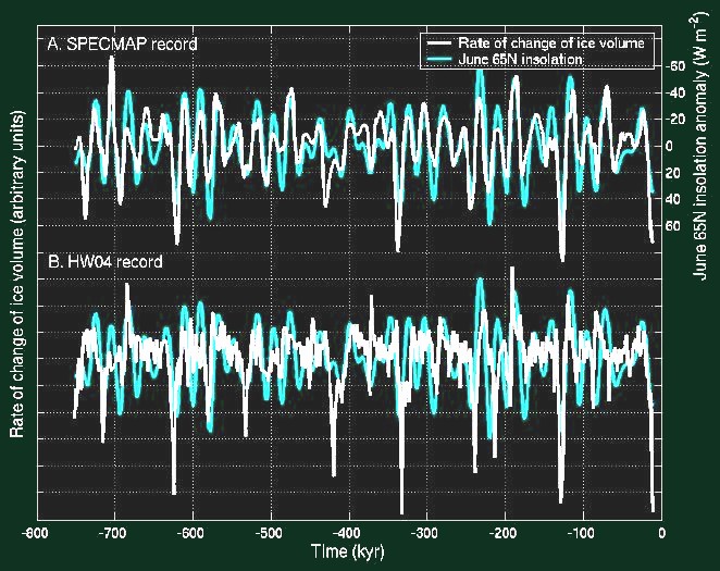

Both Science of Doom and I have discussed it and replicated it, although in our replications we we used the newer data rather than the older data used by Roe. As SoD pointed out, the top panel above (SPECMAP) used “ice volume” data that was tuned to the insolation, so it is useless.
So let me refer you to SoD’s excellent discussion, here and here, to which I have little to add.
Please note the only differences between the lower panel above and my Figure 3 in the head post are that 1) I’ve inverted the ice volume proxy data (so that warming is up); 2) I’ve used the newer Huybers data as a proxy for ice volume rather than the Huybers 2004 data used by Milankovich; and 3) I’ve used the Berger insolation data, which is slightly different from that used by Milankovitch. (The only provenance of the insolation data used by Milankovitch is “The author thanks J. Levine for providing the insolation codes”, or I would have used Milankovitch’s insolation data.) Here is my data, in the format used by Milankovitch:
In other words, I’ve repeated the Milankovitch analysis used in the lower panel. As a result, all of the figures and calculations are of the Milankovitch claims, replicated using the best and most modern data that I can find.
Regards,
w.
Willis,
In Fig. 1, you are comparing an “energy flow” variable (J/s/m^2) and a “scalar state” variable (deg C), and you’re plotting them on a time-logarithmic scale. That means that those tiny bumps near 100ky in the red curve of Fig. 1 actually correspond to 10,000s of years of having a somewhat higher influx of energy; in total, quite a lot of extra energy. The big peaks at 20 and 40 years look more impressive, but correspond to much less energy being sent to the earth. So is it entirely fair to compare the two? Basically, all the signal power near the 100ky frequency is spread over a much wider interval.
Would it not be interesting to have a binning of signal energy, e.g. add all the peaks from 0-999 into a bin, and rinse and repeat for 1000-1999, …., 100000-100999, etc., and then plot the binned signal against the average temperature over that bin?
Frank
Willis –
I wouldn’t argue that insolation at a specific latitude forces global temperature. You are on the right lines in suggesting now that temperature first differences should relate to insolation, especially when the ocean is going to take thousands of years to equilibrate at depth, i.e. response to insolation is not instantaneous.
However, the multiple orbital parameters clearly do provide a very helpful model, when you consider:
oops. When you consider:
1. Changes in *Global* insolation, forced by eccentricity changes
2. Changes in Obliquity, dictating the size of the arctic/antarctic zones
3. Changes in Perihelion, dictating the relation between the seasons and the earth’s orbit.
All of these together can generate quite a fetching fit to global temperature.
If you are trying to debunk the idea that insolation at a specific latitude drives ice ages, I’m right with you. If the broader point is that an explanation based on (Milankovitch) orbital parameters is wrong, then I think that isn’t the case. As posted before, see:
http://www.robles-thome.talktalk.net/Milank1.pdf
R.
In the geological past there was a prolong period when the Earth’s poles were free from the long term ice coverage, followed by the current glacial epoch. The cause of the change from one to the other is not clear, possibly the solar system’s passage through galactic dust clouds.
However, what is clear is that the short irregular interruptions of the glacial epoch are correctly identified by the Milankovic cycles of increase in the N. Hemisphere’s solar irradiation
As these short periods in steep temperature rises are irregular spectral analysis will not lead to correct interpretation of periodicities concerned.
Finally, the absence of the Dr. Svalgaard’s comments is regrettable.
May I summarise the comment I made in the last thread.
The pattern can be explained if one assumes the following
1) The onset of an ice age is caused by reduced insolation (MC)
2) Ice growth is accelerated by albedo changes
3) Sea ice reduces the energy lost to space so that the energy balance is POSITIVE which means that energy is stored in WARNING oceans under the ice.
4) The warming oceans melt the ice from below as the ice thickens above creating huge instability in the ice shelves
5) Eventually the sea ice calves into the warm oceans creating relatively rapid temperature fluctuations as the ice packs melt in the summer exposing the warm oceans and refreeze during the winters restoring the ice cover until the next major calving.
This pattern began to appear a couple of 1 million years ago when the Isthmus of Panama closed and became fully established 1 million years ago once the Atlantic had cooled to a critical temperature. Prior to this the Atlantic was warmed by currents and winds from the Pacific which prevented massive sea ice build up.
CAL
This is a very helpful summary, and explanation of ice sheet instability. An action causing its own reaction – this can be called “friction” and is a necessary ingredient in chaotic-nonlinear instability and oscillation.
About the Atlantic and Pacific. In Willis’ previous Argonouts post, the temp with depth animation showed that the Pacific at depths >1000m is colder than the Atlantic (and Indian) ocean. So the Atlantic is cooler at the surface but warmer at depth, than the Pacific. Is there a zero sum game here? With the heat capacity of water, and the volume of water in the oceans, there must be in the short term.
Frank Excellent point
Combine Franks comment at 4:32 1/26
“In Fig. 1, you are comparing an “energy flow” variable (J/s/m^2) and a “scalar state” variable (deg C), and you’re plotting them on a time-logarithmic scale. That means that those tiny bumps near 100ky in the red curve of Fig. 1 actually correspond to 10,000s of years of having a somewhat higher influx of energy; in total, quite a lot of extra energy. The big peaks at 20 and 40 years look more impressive, but correspond to much less energy being sent to the earth. ”
with Denniswingo at 7:18 pm 1/25 who points out
” Look at first principles. At maximum eccentricity the difference in insolation at the top of the atmosphere is well over 100 watts/m between perihelion and aphelion. That is a hell of a difference. Using average values masks these variations.”
I think this provides an explanation of the eccentricity influence.
Willis,
about the “solution” of this 100ky cycle problem (one of the many solutions), you should definitely check out Abe-Ouchi et al 2013 Nature Vol 500 Nature 8 august 2013
http://www.nature.com/nature/journal/v500/n7461/full/nature12374.html