Guest Post by Willis Eschenbach
Well, either it’s a genetic defect or I’m just a glutton for punishment, but I’m going to delve some more into the ice ages. This is a followup to my previous post, Into and Out Of The Icebox. Let me start by looking at the cycles in the insolation and the cycles in the geological temperature. I’ll use the same temperature proxy dataset used in the discussion by Science of Doom here and here, which is the Huybers ∂18O dataset . For the insolation, I’m using the same Berger dataset that I used in my last post. Figure 1 shows the cycles in the two datasets:
 Figure 1. Periodogram of the Huybers temperature proxy dataset (blue) and the June insolation at 65°N from the Berger geological insolation dataset.
This graph demonstrates extremely clearly what is called the “100,000 year problem”. As you can see, the length of the ice ages has a very strong 100,000 year cycle, with a cycle amplitude greater than 40% of the swing of the data.
But in total contradiction to that, the June insolation at 65°N, which is the insolation that is supposed to cause the interruptions of the ice ages, has virtually no cycle strength in the 100,000 year (100 Kyr) range. The insolation has its greatest cycle strength between 19 and 24 Kya, and a smaller peak at 41 Kyr, but there is almost no power at all in the 100 Kya range.
It is worth noting that both the temperature and the insolation do show power in the ~ 23 Kyr and the ~ 41 Kyr range … but only the temperature has power in the 100 Kyr range.
Now, back in 2006 Gerald Roe wrote a paper called “In Defense of Milankovich”. In that paper, he said that the reason there was little relationship between the Northern Hemisphere insolation and the ice ages was that people were looking at the wrong thing. His point was that when the sun increases, the ice doesn’t immediately disappear. Instead, what changes is the rate of melting of the ice. This is also called the “first difference” of the ice volume. Roe used an earlier version of the same Huybers temperature proxy dataset I’m using to demonstrate his hypothesis, reasoning that the ice volume is a function of the global temperature.
So let’s start by looking at the effect of taking the first differences on the underlying cycles. Figure 2 is the same as Figure 1, except that I’m using first differences instead of using the raw Huybers temperature proxy data.
 Figure 2. Periodogram of the first difference of the Huybers temperature proxy dataset (blue) and the June insolation at 65°N from the Berger geological insolation dataset.
Now, that is an interesting result. As you might imagine, it hasn’t introduced any new frequencies into the mix. However, it has greatly decreased the size of the 100 Kyr cycle, slightly increased the size of the 23 Kyr cycle, and slightly decreased the size of the 41 Kyr cycle.
And what would be the result of those changes? Well, the correlation will indeed be better, as Roe observed … but for the wrong reasons. The correlation will be greater because in the temperature data (blue) the ~ 20 Kyr cycle and 41 Kyr cycles are now about the same size as the 100 Kyr cycle. So those cycles will fit better … but we still have no explanation for the 100 Kyr cycle.
In any case, here’s the match between the June insolation at 65°N and the first difference of the temperature proxy:
 Figure 3. A comparison of the June insolation at 65°N (red) and the first difference of the ∂18O temperature proxy. I am using the negative of the ∂18O data, so that increasing values show increasing temperatures.
Looks good, doesn’t it … but it’s not. Unfortunately, this is merely a wonderful example of the human propensity for seeing patterns. If you look at parts of this, it looks like a perfect match. The problem is, humans are shaped and bred by millions of years of evolution to find visual patterns … and as a result we find patterns even where no such patterns exist. The best example I can give you is that virtually every culture has found constellations in the stars. We identify Orion and Gemini and a host of others … and despite that, the stars contain no such patterns, just a random scatter.
And when we look closely at Figure 3, we can see that in many of the cases, the blue lines are in between the red lines … in all, they seem to be aligned at around 600 Kyr BP and also around the present, but badly out of alignment in between.
In order to keep ourselves from making such mistakes in pattern identification (among other reasons), we’ve invented an entire branch of mathematics called statistics. It allows us to do things like measure just how much of one variable is explained by another variable. The measure of this is called “R^2”. It varies from 0.0 (no relationship) to 1.0 (one variable totally explains the other).
And the R^2 value for the two variables above? How much of the first difference of the temperature variation is explained by the variation in northern insolation?
Well, the R^2 of the two is a mere 0.05 … that is to say, the June insolation at 65°N only explains about 5% of the variations in the first difference in temperature. Color me unimpressed.
Now, it’s possible that there is some lag in the data. To check that, we can run a “cross correlation”. This looks at the correlation, not just at the same time, but at a variety of time lags. Here is the cross correlation of the two variables:
 Figure 4. Cross correlation of insolation and first difference of temperature. Positive lags show temperature changes lagging insolation changes. Blue lines show the level where the p-vaule is 0.05, which must be exceeded to achieve statistical significance.
So … there you have it. The relationship just barely achieves statistical significance. Is it true that looking at the first difference of the temperature improves the correlation? Yes, it is … but for the wrong reason. Taking the first difference of the temperature proxy reduces the amplitude of the 100 Kyr signal and increases the amplitude of the ~20 Kyr signal. Since the ~ 20 Kyr signal is the largest signal in the insolation, as a result the overall correlation increases … but this still doesn’t help us at all with the “100,000 year problem”. Not only that, but at the end of the day, the relationship is so weak as to scarcely achieve statistical significance.
Me, I’d say that Roe certainly didn’t solve the 100,000 year problem … although as always, YMMV …
Best wishes to everyone,
w.
My usual request—if you disagree with someone, please QUOTE THEIR EXACT WORDS THAT YOU DISAGREE WITH. This is the only way for everyone to be clear as to the exact ideas that you are objecting to.
http://svs.gsfc.nasa.gov/cgi-bin/details.cgi?aid=4249
watch video
What’s interesting about that video is that, apparently, most of the volume of the ice-sheet was laid down during the interglacial period, with considerably less left over from the preceding glacial period. Even some at the bottom left over from the previous interglacial.
More snowfall during this interglacial than during the preceding glacial period?
I did not quite understand this.
Why is there so little ice left over from the last interglacial? We are in an interglacial now, but don’t see massive melting of the ice sheet. Instead we see a massive dome of holocene ice accumulation.
If we went straight into an ice age now, we would see New Ice Age ice ice overlying a thick holocene layer. And presumably it would stay like that until the next interglacial.
Or is the ice at the bottom of the Greenland sheet constantly melting and flowing into the Atlantic?
Ralph
Glacier 18,000 years ago.
http://oi62.tinypic.com/a1pvdj.jpg
http://www.vukcevic.talktalk.net/AT-GMF.gif
As a matter of additional info for those who are not aware. The periodicity of precession is 23K years, the periodicity of obliquity is 41K years and the periodicity of eccentricity is 100K years.
As an additional reminder all representations here are based on limited data sets of temperature proxies.
@Willis:” Is it true that looking at the first difference of the temperature improves the correlation? Yes, it is … but for the wrong reason.”
Which might lead some to conclude that using first difference of temperature is ‘wrong’, betraying a certain amount of confirmation bias (i.e. looking for data which confirms our preconceived notion of how nature must behave).
Instead we should step back and look at the ‘thermometer’ itself (delta-O-18), which is the ratio of the two most common stable isotopes of oxygen in the atmosphere: O16(99.759%) and O18 (0.204%) (with O17 making up the remaining 0.037%). But the ratios are slightly different in terrestrial bodies of water and ice because the lighter isotopes bound to water molecules are more likely evaporate and subsequently precipitate back to the ground or oceans. (O18: freshwater 0.1981%, seawater 0.1995%).
It’s a rather subtle and noisy process, so not a proxy which has a simple linear relationship to temperature like mercury expanding in a tube. It’s easy to fall into the ‘engineering fallacy’, which makes us believe that all thermometers read ‘temperature’ directly from nature. It’s much more complicated than that. So to extract temperature there must be a complex model embedded in there somewhere (which have a tendency to be wrong).
So these isotopes are more sensitive to changes in state, than absolute temperature, which might explain why delta-temp correlates better than absolute T.
Note the findings of Dansgaard in 1964 (the pioneer in paleodating):
Here is something to think about. The temperature curve looks like a capacitor response to a series of charges of different voltages. The rise is rapid but the discharge can take 100k years.
“The rise is rapid but the discharge can take 100k years.”
That’s not a typically charging scenario. Charging is usually slow, discharge much faster relative to charging.
The usual model of electronic circuit which generates the cyclic slow-fast response is called a relaxation oscillator
https://en.wikipedia.org/wiki/Relaxation_oscillator
The circuit must contain at least two components 1) an accumulator (e.g. capacitor) which integrates some increasing quantity (e.g. charge) and 2) a threshold device (e.g. neon lamp etc) which fires or breaks down at some positive threshold, resetting the accumulator back to zero, creating this characteristic pattern, slow rising-fast falling</i?
http://hyperphysics.phy-astr.gsu.edu/hbase/electronic/ietron/unijun5.gif
Relaxation oscillator models fit some natural phenomena very nicely, e.g. earthquakes: strain builds up slowly then released quickly when bedrock fractures.
But the glaciation history, viewed in correct temporal order, shows a different pattern: fast-rising, slow-falling, which doesn't fit this kind of relaxation model:
http://www.brighton73.freeserve.co.uk/gw/paleo/400000yearslarge.gif
So not clear what this 'fast-rise' mechanism is. A time-reversal of discharge seems to be like a time-reversal of an explosion (which violates some laws of thermodynamics).
But a fast-rise of temperature per se doesn’t necessarily violate physics if there is hidden or latent agent causing it.
Just saying.
Perhaps your charge and discharge are inverted. The ‘charge’ is the slow accumulation of ice during the glacial. The ‘discharge’ is the sudden melting of the ice.
I see no reason why you cannot accumulate negative energy (coldness) rather than positive energy (heat). It the same process. You are just springing back to the ‘norm’ (interglacial), from an unnatural state (ice age). You can either compress a spring, or extend it.
R
“Perhaps your charge and discharge are inverted. ”
Yes, I realized the same idea while reading Craig Loehle’s post below,but with the break in the Bering Dam causing the ‘discharge’ and the rebuilding of the dam over several cycles as the ‘charging’.
See http://wattsupwiththat.com/2015/01/24/the-icebox-heats-up/#comment-1843647
Actually in fluids we have this type of response with a flap valve inlet to a reservoir and a small outlet. The reservoir fills quickly when pressure pushes the flap valve open, and drains slowly when the reservoir drains through the small hole. Like dams on rivers, fast fill, slow drain. Many similar devices in hydraulic systems. Or consider a modern electric drill. Half hour charge, several hours of discontinuous use.
What is the inverse of temperature? Maybe we are measuring the wrong parameter.
My take is that the Milankovitch parameters are sometimes a “trigger”, but the major 100kyr event is some type of ocean-current/atmospheric dynamic + ice-sheet dynamics + albedo feedback. A complex, non-linear juxtaposition of effects.
There, solved the problem. 🙂
What about the Earth’s magnetic field?
Is the Earth’s magnetic field reversing now? How do we know?
Measurements have been made of the Earth’s magnetic field more or less continuously since about 1840. Some measurements even go back to the 1500s, for example at Greenwich in London. If we look at the trend in the strength of the magnetic field over this time (for example the so-called ‘dipole moment’ shown in the graph below) we can see a downward trend. Indeed projecting this forward in time would suggest zero dipole moment in about 1500-1600 years time. This is one reason why some people believe the field may be in the early stages of a reversal. We also know from studies of the magnetisation of minerals in ancient clay pots that the Earth’s magnetic field was approximately twice as strong in Roman times as it is now.
http://www.geomag.bgs.ac.uk/images/dipmoment.jpg
http://www.geomag.bgs.ac.uk/education/reversals.html
While the Milankovitch cycles suggest a good place to look for ice ages, we my be making the same mistake the warmers are making – looking in the wrong place. We know there is a some 400 year cycle that we think is linked to sun spots. Could it be the the 100,000 year cycle is also linked to the sun? It’s possible that in warmer times, the sun burns hotter causing waste build up in the core. The cooler time are the result of the waste products mixing with new fuel for another cycle. The time it takes for the heat to reach the surface could also explain the lack of neutrino issue as well because we could still be receiving the heat from the last warm cycle long after the last neutrino peak was reached.
Just a thought reached with far [too] little knowledge of how the sun works.
Last I heard, it take a photon 100,000 years to make its way to the surface. Could a fluid body 860 thousand miles in diameter have a 100 ky cycle? 14C has too short a half-life to tell us. 10Be from ice cores would go back maybe 6 or 7 cycles, but I haven’t come across any yet googling the images. If we find a long Beryllium records (perhaps from sediments) Willis could run his periodicity program and solve the problem.
Currently (and recently) storms have been observed on Saturn and Uranus. It is impossible to say if these storms are out of the ordinary or a result of better or ‘for the first time’ observations. However, it is interesting if we are supposedly seeing an increase in storms here and also on Saturn and Uranus. That is assuming what we have on earth is an increase as opposed to many more people living in harms way. Perhaps the trigger for more storms may not be the peaks or troughs of the suns output but the change? Just thinking.
These are great blogs.
Willis The insolation at 65 N is driven by earths precession and obliquity – there are coincident temperature pekas of relatively small amplitude. The 100000 year temperature peak is obviously related to the eccentricity. You need to include in the plot the changing insolation at the equator or intra tropical region. The climate represents the effect of all three orbital parameters obviously the 100000 year periodicity in the ice ages is mainly eccentricity driven. Where is the mystery?
+1
Dr. Page is makes a good point. The eccentricity is different from the other Milankovitch cycles in that it actually alters global average insolation . That has a much more direct impact on global climate than insolation in a particular area at a particular time of year. So it is hardly surprising that a signal shows up there. There is not just one factor that controls everything.
The only 100 kyr mystery is that the insolation variation due to eccentricity is just 0.45 W/m2, just 12% of doubled CO2. Almost like there might be some sort of amplification.
I thought that obliquity was just an apparent consequence of precession. Obliquity on its own cannot exist, a planet cannot rock forwards and backwards. So counting obliquity and precession is like counting the same thing twice ?
Willis See green curve in Fig4 at
http://climatesense-norpag.blogspot.com/2014/07/climate-forecasting-methods-and-cooling.html
Note approx. 400000 year periodicity which has been identified in the geological record going back 400 million years.
Unable to find any reference to 400kyr power in the link. Strange comparison of Miocene and Hollowscene ™ power spectra that ignores the Pleistocene?
Gymnosperm See FSg 4 look at the pattern on green curve . simplest illustration – see amplitude peaks at 600,000 and 200000. – go on forwards at about 200000 year intervals – Actual intervals vary about some central mean. say 395 – 405 thousand. +/-
Gymno — the point was simply to show that similar periodicities are found in a Miocene section.
The 400000 year periodicity has been seen in the Silurian. The point is that these basic periodicities have been stable and affecting the climate for hundreds of millions of years.
Sorry comment should read go forwards at approximate 400,000 year intervals
I agree completely, Willis. With your observation that you love pain, that is.
I do find it intriguing that somebody would consider the derivative of the temperature to be the important signal when in fact the derivative of the temperature is not the temperature. In essence what one must conclude is that there is a BRIEF INTERVAL where the temperature increases quickly in the 20-30 ky range or periodicity, but that it doesn’t last long enough to actually melt anything, while at 100 ky it warms as about the same rate in spite of having almost no driving at 65 N but the warming lasts long enough to increase the temperature substantially. Say what?
In actual fact, nothing “orbital” is this sharp. We’re talking 1000-2000 year intervals here, and again in actual fact the planet can warm an enormous amount in 1000-2000 years. If ice cores are to be believed, it can warm by 5-6 C in as little as a 100 years, and that is on the SLOW part of the cycle, e.g. the start of the last interglacial. And then there is the Younger Dryas, the Eemian peak, and more.
In the end, the 100 ky “problem” remains, the countervariance of annual insolation and annual temperature problem remains, the “cause of the Little Ice Age” problem remains. None of the explanations are particularly plausible and none of them hold statistical water — the best that can be said for them is that they are possible, except when even that is denied them.
rgb
How about some side effect of magnetic fields being a factor ? Vukcevic’s Polar temperature graph is intriguiging, you (rgb) produced a co2 versus temperature graph with a 67 year harmonic, the Suns corona has a 67 year period, which is surely a result of a magnetic field. Do glaciations tie up with magnetic field excursions / reversal ?
Very unlikely since there isn’t correlation with the Earth’s reversals. Houever there is strong correlation between solar activity and Jupiter/Saturn magnetosphers’ orbital interactions. Since both Earth and sun have regular reversals it is possible that the two gas giants occasionally do have magnetic reversals as well, which may of may not be synchronous with some of Milankovic cycles. If such do last for a milenia or longer the solar magnetic activity would have a very long type of Maunder Minimum, and if so an ice age might follow but in both hemispheres simultaniously. Outer planets magnetic fields have been measured only in recent decades so above is.clearly in the realm of speculation.
Since earth enters ice houses about every 150 million years, a cosmic cause is indicated, as per the galactic arm hypothesis of Shaviv, et al. Once out of a hot house into an ice house, other terrestrial & ET factors determine just how much ice there will be, such as the position of the continents. Major ice sheets didn´t develop during the Mesozoic (Jurassic\Cretaceous) ice house, for instance, as did occur during the two Paleozoic ice houses.
Once in an ice house phase, it is pretty well understood how glaciation happens. Snow that falls in winter doesn´t melt in summer. Over tens of thousands of such summers, you get not just more montane glaciers but vast domed ice sheets. High latitude insolation changes are IMO strongly implicated in starting ice ages in this sense of the term. Milankovitch cycles account for the 40 Ka periodicity at high statistical levels.
Why I see little problem for Milankovitch theory in the longer periods of glaciation in the latter Pleistocene is that the 40 Ka cycles don´t go away. They´re still there & still well explained by insolation. It´s just that they now occur within longer periods of glaciation. They cause the ice sheets to wax & wane. If there´s a problem, it´s in showing what caused the longer cycles within which the shorter ones still operate. IMO obliquity & eccentricity do it, along perhaps, as noted above, with increased albedo due to more ice as the planet cooled during the first half or so of the Pleistocene.
denniswingo
January 24, 2015 at 11:36 pm
“There is another thing that bothers me about these types of analyses. It assumes a perfectly round and perfectly flat Earth. At sea level the instantaneous insolation is about 1000 watts/m2. At 6,000 feet that number is closer to 1175 watts/m2 and at 10,000 feet is closer to about 1250 watts/m2. The northern hemisphere at higher latitudes is at a much higher altitude than the southern hemisphere at the same latitude.”
Willis Eschenbach
January 25, 2015 at 1:17 am
denniswingo January 24, 2015 at 11:36 pm Edit
Willis, I believe the point of denniswingo’s comment is that the topography of the ice sheet is in play (not just the mountains). A three km high ice sheet, like a mountain, is going to still be freezing on top despite the insolation (a large amount of which is also going to be refleccted back. I think a missing factor here is the following: During much of the latter part of glacial period, the relative humidity is very low (which attenuates accumulation) and perhaps a good part of ice reduction is by sublimation with little part played by insolation.
A number of other factors are at play as well. As the ice thins there is a certain amount of crustal rebound partially maintaining altitude of the the top of the ice sheet, increasing humidity, rising sea levels, all without a strong correlation to insolation. Anyone up to calculating how long it would take to reduce the ice thickness, say to half, by sublimation at a realistic temperature profile for the period? After all, Kilimanjaro showed a significant difference in a decade or so.
The following are in your face Milankovitch cycle theory killing deficiencies/failures which unequivocally support the assertion that insolation at 65N does not and cannot physically cause the glacial/interglacial cycle. The theory that insolation at 65N ’causes’ the 100,000 year glacial/interglacial cycle (note the glacial/interglacial cycle was a 41 kyrs period from 2.6 million to 1 million years ago and then suddenly for unexplained reasons to changed to a 100,000 years) is a Zombie theory.
A Zombie theory/mechanism generates piles and piles of anomalies and paradoxes but is still kept alive as the correct solution is not known which makes it impossible to kill the Zombie theory.
Field after field of science have Zombie theories which generate piles and piles of anomalies/paradoxes.
http://en.wikipedia.org/wiki/Milankovitch_cycles
This recent finding that the planet cyclically abruptly cools both poles should have been the final stake in the heart of the Insolation at 65N theory (Do you get that insolation in the summer is maximum in the Southern hemisphere when it is minimum in the Northern hemisphere?), but somehow the insolation at 65N still lives in the imagination of the public and the warmists.
http://earthobservatory.nasa.gov/Newsroom/view.php?id=24476
Don’t forget that because Earth’s orbit is elliptical the orbit speed is increased at perihelion. As eccentricity increases the Earth spends less time close to the Sun not only due to the path of the elliptical orbit but also because it is traveling faster through the orbital path when close to the Sun. More time farther from the Sun, less insolation at the surface. Lower obliquity during a higher elliptical orbit enhances the effect. The only times that Earth has entered an inter-glacial over the last 800k years is when eccentricity is low, obliquity is high and NH summer solstice is at perihelion. Whatever the proxy temps say, whatever the charts depict, whatever the whatever, there is no doubt the inter-glacials happen at certain times when orbital parameters are just right. Whether that is the cause or whether that is causing something else is the question.
Here is my understanding of how this could work. One of the key factors in an ice age is the freeze up of the Bering straits, which then prevents circulation of water into the arctic. This is gradual as water level lowers and ice increases (gradual cooling) but when it gives way it is more sudden and the ice begins to melt rapidly. These processes are threshold events and take a very long lag to get to. They are related to northern hemisphere insolation but also to total ice volume which lowers sea level and makes the straits more of a barrier.
Sandal, C. and D. Nof. 2008. The collapse of the Bering Strait Ice Dam and the Abrupt Temperature Rise in the Beginning of the Holocene. J. Physical Oceanography 38:1979-1991.
Thinking along similar lines, Ewing & Donn, two of the world’s leading oceanographers back in the late 50’s, hypothesized that rising sea levels at the end of the last inter-glacial led to an increase in warmer water flowing into the Arctic Ocean, causing it to become ice-free and providing a rich source of moisture for the atmosphere to draw on. Moist surface winds blowing towards Northern Canada, Europe and Eurasia then bought the snows which enabled the ice sheets to start forming :
http://strongasanoxandnearlyassmart.blogspot.co.uk/2011/07/scientists-predict-another-ice-age-is.html
Maybe the alarmists are actually right, to hyperventilate about the possible loss of Arctic Sea Ice, even if it is for entirely the wrong reasons!
Yes. Noted this also in a comment to previous thread. And YD was almost certainly ice dam related also. The resulting meltwater pulse interrupted North Atlantic thermohaline circulation.
As a gedanken experiment, the Malasian air crash is in 30 meters of water at the center of the strait between Malaysia and Borneo. At the peak of the last glacial about 20 millenia ago sea level was about 120 meters lower. That part of the western Pacific would have been dry land, including the entire Strait of Malacca with maximum depth 37 meters. So ENSO would have been different. Pacific currents would have been different. We know the Gulf Stream at the Florida Strait was significantly weaker at the last glacial maximum. (Nature 402: 644-648 (1999)) It is quite possible that the main climate mode for the past million years is ‘glacial’, but after enough ice mass builds and sea level drops some ocean threshold is crossed that increases poleward heat transport from the tropics causing the fairly sudden (about 10-12 millennia) melt into an interglacial. Henry’s law and Le Chatelliers principle would make CO2 a positive feedback to that per ice cores, with a lag on the order of 800 years. (Gore had it backwards. CO2 lags.) Sea level rise, CO2, albedo, etc, eventually ‘stabilizes’, poleward heat transport ‘renormalizes’ and the process starts over, with growing ice sheet albedo being a significant cooling feedback factor. Just a gedanken.
The Bearing Strait is not the full answer.
The Ice Age ‘breaks’ and ends just when it is reaching its maximums, not when it had already started melting. There is no mechanism I can see that would ‘break’ the Bearing Straits dam, while the Ice Age is still at its peak.
Ralph
William states “Orbital eccentricity’s impact on 65N insolation is the smallest of all the orbital parameters yet for some unexplained reason the glacial/interglacial cycle follows a 100,000 year cycle. Note the glacial period ends when the Northern hemisphere is closest to the sun in summer which occurred 11,000 years ago. The Southern hemisphere is currently closest to the sun during the Southern hemisphere summer (opposite to the orbital position 11,000 years ago) which is the position to terminate interglacial periods.”
Link below for this interesting walk on the wild side…”In examining the phenomenon of the precession of the equinox (which was the original impetus for the development of lunisolar precession theory) we have found that a moving solar system model is a simpler way to reproduce the same observable without any of the problems associated with current precession theory. Indeed, elliptical orbit equations have been found to be a better predictor of precession rates than Newcomb’s formula, showing far greater accuracy over the last hundred years. Moreover, a moving solar system model appears to solve a number of solar system formation theory problems including the sun’s lack of angular momentum”….
http://www.binaryresearchinstitute.org/bri/research/evidence/lunarcycle.shtml
…”Under the current lunisolar theory of precession it is assumed that the earth goes around the sun 359 degree 59 minutes and 10 arc seconds in a Tropical year, the period from like equinox to like equinox, which is equal to 365.2422 rotations of the earth. This is true if you measure the position of the equinox relative to the fixed stars “OUTSIDE” the solar system but it is not true if you measure the movement of the equinox relative to the sun or moon or other objects “WITHIN” the solar system, where the lunar data shows us that the earth goes around the sun a complete 360 degrees in a tropical year. Unfortunately, neither NASA VLBI nor any other official agency measures the earth’s orientation relative to nearby objects, so the paradox goes unnoticed”…
Does nothing to explain why the cycles we measure, but certainly would relate to why we find no correlation in the climate record.
Of course, the Earth’s climate has been following cycles of cooling and warming, throughout it’s history. Now we are living in the holocene era, a period of gradual warming of the climate, following the ice age, which has ended over ten thousand years ago. Some are saying that the climate is changing in a more rapid manner startig with the 20th century, mainly because of human influence. The greenhouse emissions are the most pointed cause of climate change, especially global warming. Some other theories exist, however, which point to the oceans, which are considered to be the main influence on global climate. The two world wars of the past century, especially the naval battles are thought to have had an important role in changing the climate. Have a look at http://www.warchangesclimate.com/ for more info on the matter.
Has anyone tried to correlate temperature variations (or some portion thereof) with the impact of episodic glacial meltwater releases? I know there is research concerning the AMOC as well as the Bering Strait and how they influence (and are influenced by) global climate and freshwater discharges. It would seem plausible that freshwater pulses (and the specific timing of major releases) could interact with both oceanic currents and high latitude insolation to mask any single influence’s precise impact. Major freshwater releases have abrupt tipping points (dependent upon local topography) that would not necessarily coincide with orbital cycles. For example, if freshwater pulses changed in frequency, volume or both, perhaps there is a non-orbital mechanism for shifting between 41k year and 100k year cycles?
In any numerical analysis, before even getting into the numbers, I always want to know how accurate the numbers themselves are and what assumptions went into generation of the numbers. So before beginning an analysis of cyclicity of past glaciations, I’d like to know the basis for data making up ‘geological temperature swings’ and what assumptions went into generation of those numbers. In a response to Willis’s earlier post, I pointed out some of the problems with these numbers. In a nutshell, we can date the last two glaciations (back to a few hundred thousand years) with various istopes (14C, 10Be, 37Cl, U series, and others) but the older glaciations are not directly dated. Since the direct dates we have are from glacial moraines, we know when they occurred, but don’t have temperature measurements. For those, we have to rely on ice cores and deep sea cores, but the problem here is they are not directly dated and their ages are inferential with lots of built in assumptions.
In addition to the dating problems, what assumptions are built into the numbers? In a word, a lot (see my response to the previous post). That doesn’t mean the numbers are wrong, but it does mean that if the assumptions aren’t valid, neither are the numbers. What I’m trying to point out here, is that Willis’s analysis, is as usual, elegant, but the sources of the numbers for ‘geological temperature swings’ are really not very robust for the older glaciations.
Aside from the statistical analyses, there are very serious problems with the Milankovitch theory. For example, (1) as John Mercer pointed out decades ago, the synchroniety of glaciations in both hemispheres is ‘’a fly in the Milakovitch soup,’ (2) glaciations typically end very abruptly, not slowly, (3) the Dansgaard-Oeschger events are so abrupt that they could not possibility be caused by Milankovitch changes (this is why the YD is so significant), and (4) since the magnitude of the Younger Dryas changes were from full non-glacial to full glacial temperatures for 1000+ years and back to full non-glacial temperatures (20+ degrees in a century), it is clear that something other than Milankovitch cycles can cause full Pleistocene glaciations. Until we more clearly understand abrupt climate changes that are simultaneous in both hemispheres we will not understand the cause of glaciations and climate changes.
I have to agree 100% with this. My geology degree is long in the past, but I enjoy reading articles and books regarding the Ice Ages and the standout feature, without a doubt, is the extreme and rapid climate instability during the Ice Ages. Dansgaard-Oeschger and Heinrich events occur in the blink of an eye in geological terms and in the case of the YD we are talking a decade or two. These types of changes are far beyond anything witnessed by anyone today. In retrospect the Holocene is a time of extreme climate stability compared to the previous 100,000 years. And that is a very sobering thought.
My viewpoint as well. The temperature spikes, known as interstadials, throughout the Pleistocene have been sudden. The D-O spike was the same. The YD stepdown was typical, though we have much better resolution on these nearer events than the older, less well resolved events as recorded in the ice cores.
It should be said that Don Easterbook is a professor emeritus in glaciology.
Yes, I know that Don is Dr. Easterbrook, PhD Geology, which is why I enjoy his commentary and articles.
As an aside a memorable moment for me was when our resident palynology expert, the late Dr. Bill Matthews of UBC, took us students to an area near the mouth of the Fraser River to take a core of the peat bog. The core was around 5 meters (15′) in length and consisted, as expected of peat which abruptly ended in sand which marked the start of Ice Age deposits. For a geology student this abrupt change was unforgettable, plus the fact that Bill Matthews told us that the lower layers contained Oak pollen which indicated a warmer and drier climate in the early Holocene. Seeing all that in a peat core was amazing.
E. J. Mohr:
No question, the Holocene started quite abruptly and ice core data shows this clearly. Other proxies do as well, as in your example.
It’s as if someone ( who?) threw a switch.
Here allow to demonstrate…[click]…
See?
>>oak pollens
The oak pollens at that latitude demonstrate that this was a much warmer climate, at a time when the ice sheets were still present (but melting).
The M. Cycles cannot explain this, because the M.C.-induced insolation levels are up and down all over the place – while the ice sheets are doing something completely different and completely disconnected to the changes in insolation. The Ice Age is often still busy growing ice sheets, while insolation is at its absolute peak.
.
The answer to the 100,000 year Ice Age conundrum has to lie in something like a radical change in cloud cover – something that can protect the surface from increasing M. Cycle insolation, and keep the summers cool. All you need is a string of summers with temperatures below that required to melt all of last winter’s snow, and you have just begun the process of a new Ice Age. And this will continue, for as long as the excessive cloud cover persists.
However, when you reach the point at which the clouds part and disappear (for some reason), then you can indeed have really baking hot summer temperatures, with majestic oaks growing next door to some huge (but rapidly retreating) ice sheets.
R
The real paradox is albedo. Just when glaciers reach their maximum extent, and albedo reaches its highest, everything starts to melt. Makes one wonder how much albedo really counts.
Palynology is wonderful stuff and I wonder why you don’t see any climate reconstructions based on such studies.
An infallible way to second varves, tree rings, etc. or so it seems.
Methinks the switch may have had an embedded link, but she no work for me. Meanwhile where I sit in SE BC I can look out the window and see the Holocene Neo-Glacial ice on the mountains. I can see all the moraines that indicate the LIA and possible earlier ice advances. The mountains tell a very interesting story, but that is not all.
The palynology and midge data from the lakes tells us that the Interior Wet belt forest that exists here may only be around 2500 years old. Prior to 4000 years ago the forest type was different – mostly spruce and pine which indicates a warmer drier climate. In southern BC the lake sediments in the upper Ashnola River speak of much warmer climate with frequent forest fires. So, the idea of static climate is a very bad idea, as the evidence does not support it. Getting back to the Ice Ages I certainly agree that the changes are so sudden that is indeed as if a switch was turned on or off. And that is where the problem starts.
Hi E.J Mohr
“So, the idea of static climate is a very bad idea, as the evidence does not support it. Getting back to the Ice Ages I certainly agree that the changes are so sudden that is indeed as if a switch was turned on or off. And that is where the problem starts.”
——————-
There is an explanation for that fast switch turn.
Is only an illusion created by the certainty given to the length of the Ice Age, the 100K years long.
You see in a scenario of a much shorter length that will not be the case.
You can not say the same thing if glacial periods only 5K years long.
It seems fast and quick only because of the long length of the glacial periods, which very well could be a very wrong estimation.
Basically it is estimated that way because the ice core data temp record is considered and interpreted as a true representation of the global climate temp variation. The temp signal in the ice core data is considered as the true signal of climate.
That is what happens when M. Cycles theory “marries” the ice core data……. they prove each other and as a result we get a wrong picture (borne) of climate and climate change and we end up considering the polar regions variations and temp records as a true representation of climate change, wrongfully.
You see if we were to estimate the climate and the GW for this last century by relying in the polar Arctic temp records, we be already in a very quick strong and a runaway GW.
The arctic did warm much more than what was projected even from the Runaway Global Warming theorists.
In same time the climatic global picture was different.
Relying in Arctic temps shows that we already must be in a AGW.
That is the distortion of Polar regions records and data while recording the climatic impulse, in too far and a too wide error.
The latest adjustment of Y.D is simply because even it is too exaggerated due to the distortion effect of the ice core data.
cheers
whiten – I was speaking of lake sediment data in British Columbia during the Holocene where already we see that climate is not static, and all this during the benign Holocene. As far as orbitally tuned data, well Don Easterbrook has already explained that the method of tuning using M-cycles will skew the results so that you cannot help but find the M-cycles. OTOH as TTY pointed out on another thread there is no really good way to date sea bottom cores, and kilometres of ice, where the annual layers are impossible to discern. Until a better solution is found, if ever, we have to go with this, bearing in mind that it may be wrong.
But all is not lost since there are terminal moraines at the southern extant of the NA ice lobes that have been dated and they match with the 100 ky cycles. There is also the famous Devils Hole Cave and other caves that provide independent, and non tuned data. The end result is that, although science is not settled, I think we can safely assume for now that the last Ice Ages have been on a 100,000 year cycle with brief interstadials like now. The mystery is still – how and why do Ice Ages end, and how do they start? M-Cycles don’t seem to provide enough solar variation for either process.
E.J. Mohr
January 25, 2015 at 10:30 pm
“The end result is that, although science is not settled, I think we can safely assume for now that the last Ice Ages have been on a 100,000 year cycle with brief interstadials like now. The mystery is still – how and why do Ice Ages end, and how do they start? M-Cycles don’t seem to provide enough solar variation for either process.”
———————–
Hello Mohr.
Thank you for your reply
Let me explain my point again in regard to your statement above.
First, please do understand that I am very aware and clear about the possibility of my arguments to be completely wrong…but this said, I would like to explain a bit further my point.
The length of the glacial periods (Ice Age) as far as I can tell is estimated as 100K years long in accordance of the temp records of the ice cores.
So the ice core data is considered as a true representation of the climatic change because of the polar regions do drive the climate through a cooling period (causing the cooling period) due to the ice build up in the polar regions because of the M. Cycles effect.
So the ice building up in the polar regions causes the the climatic cooling ( Ice Age) as explained through the M. Cycles theory.
So when you say M. Cycles don’t seem to provide enough solar variation for either process…. you lose the 100.000 year glacial period,….. the ice core data at that point is not anymore a correct representation for the length of the Ice Age.
So the length estimation of the glacial periods is at 100K years long only while the ice core data in “marriage” with the M. Cycles effect as a cause, otherwise that estimation becomes completely arbitrary and bears no mark of certainty, but in contrary becomes very dubious and confusing.
The only way to explain the discrepancies between the ice core data and the M. Cycles effect are two possibilities:
1- The M. cycles effect simply good enough (or strong enough) only to trigger the glacial periods and “drive” the glaciation to a point and then fail to drive climate change any further.
2- The M. Cycle effect not good at all to cause or trigger any climate change, but strong enough to drive the extremity behavior of the polar regions during given climate states.
This will mean that the ice core data still represents a climatic signal in the temp records but very much distorted.
In both these cases a new glacial length estimation required, as the current estimated one will be in a very high possibility to be wrong..
Please understand my point.
There is not a fair and a correct ( considered as possibly true) estimation of a glacial period at 100K years long if M. Cycles theory debunked or not considered as the explanation for the Ice Age(s).
There is no any glacial cycles or Ice Age cycles or Interglacial cycles.
All these are periods. If there is any cycles it will be climate cycles which will be made up of glacial periods and Interglacial periods.
And a climatic cycle with a 15 K years Interglacial and a 100K years Ice Age is a very much distorted cycle.
Thanks again for your reply, …….just furthering a bit more my argument…..very possible that I could be wrong…
cheers
whiten – if I understand you correctly you are uncertain as to whether or not Ice Ages actually last 100 kilo years vs interstadials which average a mere 10,000 years. You have correctly deduced that orbital tuning may make the data look like this when, in fact, it could be very different.
As far as I know the southern margins of the continental ice sheets in North America have been dated via non orbitally tuned techniques, using the actual terminal moraines as far as I know, and these tell us that the last two ice advances that were about 100 kilo years apart. So, even without ice cores or ocean sediments we have an independent age calculation. There are also speleothems that give non orbitally tuned data, so again we have reason to believe that the 100 kilo year signal is real. I hope that helps.
E.J. Mohr
January 26, 2015 at 9:24 pm
Yo say:
“whiten – if I understand you correctly you are uncertain as to whether or not Ice Ages actually last 100 kilo years vs interstadials which average a mere 10,000 years. You have correctly deduced that orbital tuning may make the data look like this when, in fact, it could be very different.
————-
Hello Again Mohr.
Thanks again for your reply.
Hopefully you be reading this.
Now , as per above selected part from your last reply to me, I want you to know that I am very certain of the high probability of the possibility that the 100K length of a glacial period is a wrong estimation.
Whether I am wrong or not with that is entirely another matter, but to be honest I have no doubt of it’s fallacy, as the things stand.
Now going further with the rest of your reply.
You say:
“As far as I know the southern margins of the continental ice sheets in North America have been dated via non orbitally tuned techniques, using the actual terminal moraines as far as I know, and these tell us that the last two ice advances that were about 100 kilo years apart. So, even without ice cores or ocean sediments we have an independent age calculation. There are also speleothems that give non orbitally tuned data, so again we have reason to believe that the 100 kilo year signal is real. I hope that helps.”
————
Keeping with as far as you know and with as far as I know, and not trying to doubt and argue the accuracy and the precision of the method in question, as per above, but only taking it in the face value that is of the most higher probable precision and accuracy, even then there still seems to be a big problem with it as a proper correct valid and indisputable evidence for the 100K years length of the glacial periods.
The first problem is that it can be clearly shown that is not even better than the ice core data, while it is considered as a kind of proof or evidence of the length of the glacial periods, in the very way you are suggesting.
Even with total rejection of the M. Cycles theory, still ice core data shows clearly that for the last 400K years there has been 4 significant ice advances with a frequency of been apart in the ranges from 80K years to 100k years.
I don’t know of any one including me who argues that.
Now coming back to the other evidence that you offer as per above.
When said that “the last two ice advances that were about 100 kilo years apart”, ……actually trying to use the numbers correctly, that will be only considered as ~100kilo years apart, which while considering a 100K years possible length for a glacial period will be more properly represented as a range of 80K to 120K
years apart, and that at a very high precision of the method and measurement.
At that point is simply “saying” and confirming whatever the better record of the ice cores is already” saying”
So while ice core data move from the position of a “conclusive” evidence to a “circumstantial” evidence once the M. Cycles effect not considered as a cause of glacial periods, still ice core data is even better than the one you try to offer as a valid explanation for the glacial length, in the way you do.
So the evidence you offer is only another kind of a circumstantial one and weaker too.
In another way, for the clarity of the argument, if ice core data without the support from the M. Cycles effect move from a 90% probability to 50% PROBABILITY of accurately estimating the 100K years length of the glacial periods, then the other method you offering above fairs much worse, somewhere at 30% probability.
Also, a simple conclusion as put above from you;
“and these tell us that the last two ice advances that were about 100 kilo years apart. So, even without ice cores or ocean sediments we have an independent age calculation”
—
means that the total independence of the age calculation (as per above) from other evidence, like from the ice core data, can only give you an estimation of the length of a glacial period as from ~50k years to ~100K range, with a huge error margin, in any possible definitions of the meaning for “ice advance”.
Further more, for the “evidence ” you offer above to be of any significant meaning and considered as possible to estimate the length of the glacial periods at a 80K years to 100K years range, in its own alone it needs two main Ingredients:
1-The very high precision of the method and measurement used.
2-The very high precision of the climate cycles to be considered.
So even while considering the method and the measurement as of a very high precision, still we need to have the climate cooperate and be to an accuracy of its cycles with the precision of a Swiss clock, meaning that the repetition of the ice advance will be at the precise pattern for any glacial period at any given moment, otherwise the estimated range will be too wide and wider for a wider glacial period.
With a 15k years Interglacial followed by a 100K year supposed glacial period the climate supposed cycles will be anything but not precise, too far distorted, far removed from the possibility of a very high precision cyclic repetition.
Using only ice core data as the data stands, without any further interpretation nearly the same could be claimed, as you claim in your reply to me.
While in the case of ice core data one can cherry pick and show advances of ice every 80K ,100K or 120K year apart, or showing two significant ice advances in the same glacial period at about 80K years apart…..in the case of what you offer the thing is so lose lose that whatever done no one can be blamed of any cherry picking as there no any clear reference.
So in the end of the day, in my opinion, the ice core data is much better than one you offer but still not good enough when M.cycles theory not considered and rejected. That’s how lose lose the evidence you offer is, especially when trying to stand in it’s own “feet” as of some meaning.
Please do forgive me if in the end of the day this argument of mine ends up to be just a result of a figment of my imagination, but only speaking up my mind here, in hope I learn something new.
Thanks again for your reply.
If you read this please offer some feedback to me by replying, if you would not mind…..
Appreciated
cheers
whiten – I suggest you look at the Devils Hole Data which independently corroborates the ice core and deep sea drilling data. Based on that I can say that the length of the Ice Ages is not in doubt, and we can be very confident about that. I would ballpark it as 90% certain or better. There is some wiggle room, but there is very little doubt that the last million years have been mostly cold. The Devils Hole project is here:
http://pubs.usgs.gov/fs/2012/3021/pdf/fs2012-3021.pdf
Now if you accept the data, and I do, then the problem really comes down to how this whole business of Ice Ages and Interstadials comes about.
E.J. Mohr
January 27, 2015 at 1:08 pm.
Thanks.
Your reply very appreciated.
Very helpful link there.
While the paper goes to a fair length of explain the probable fallacy of Milankovitch theory still I can’t find any thing that it can really support in it’s own in regard of the length of the glacial periods.
The main contribution of Devils Hole Research to the paleoclimatology is the debunking of the Milankovitch cycles, which you know I am not arguing.
Also its further contribution consist mainly about the interglacials and still there nothing much about glacial periods.
Let me brink some copy paste as to explore this in more detail:
From the paper The Devils Hole oxygen-18 :
—-
1-“The Devils Hole oxygen-18 time series is
primarily a proxy indicator of paleotemperatures. Unlike oxygen isotopes in deep-sea cores, it is not a record of past global ice accumulation in terrestrial systems. Rather, the time series
appears to correspond, both in timing and relative magnitude,to variations in paleo-sea-surface temperature…….etc. ” (self explanatory)
2-“The Devils Hole record is also highly correlated with major variations in paleotemperatures recorded in the Vostok ice core from the East Antarctic Plateau”
And the third one below is the only time when glacial periods may have being mentioned while in the point of trying to debunk the M.hypothesis :
3- “The high correlation between the Devils Hole record and the ice core record at Vostok on the East
Antarctic Plateau indicates a consistent interhemispheric timing of Pleistocene ice ages, which also is not consistent with the Milankovitch hypothesis.”
——-
So either I am missing something or the paper is not saying much at all about the length of the glacial periods.
Then according to the copy-paste number 2 and 3 the high correlation claimed with Vostok is simply of a supportive nature to that ice core data in the estimated timing of the glacial periods and also to a degree it gets back some support from that ice core data for its own validity and accuracy as a proxy indicator of paleotemperatures.
Again the ice core data is a much stronger evidence than the one mentioned. The paleoclimate data is heavy effected by the ice core data more than FROM any thing else, as far as I can tell.
Besides there is a probable logical fallacy in the way that you may read and interpret the above when considering the “high correlation”.
So to speak the ice core data are considered beyond any doubt as “polluted” or “distorted” to a degree by M.Cycles effect.
They get “polished” before considered as paleoclimate data or accurate paleotemperatures,.
You see the real temp ice cores record swings between the glacials and interglacials are at about
8C to 12C, but it is adjusted to half of that when considered in what it means in real climatic terms, somewhere at about 4.5C to 6C.
So trying to squeeze from that paper more than it actually says and claims it creates the problem of much higher supposed correlation where M. Cycles do somehow end up to have a “polluting” and distorting effect in that Devils Hole temp proxy record too..:-)
I accept that record for what it seems to me to be, probably very much so that we may diverge at that point.
In the end I can’t rate it as more than another weak circumstantial evidence still inferior to the ice core data.
But that is me at this point, probably wrong.
Thanks again for the link.
First time I read that paper, thanks to you. Pleasant.
cheers
Astley:“A Zombie theory/mechanism generates piles and piles of anomalies and paradoxes but is still kept alive as the correct solution is not known which makes it impossible to kill the Zombie theory.”
The solution to Zombie theories is sometimes as simple as finding a better reference frame to interpret data which has been correctly collected, but just misinterpreted. A classic example is the apparent ‘motion’ of stars and planets in the sky. The Zombie theories from ancient times tended to invent complicated ‘supernatural’ events and entities to explain the celestial movements. But even in more recent history, Ptolemy’s Epicycles were based on correct observations, but he just used the wrong reference frame.
Imagine trying to reconstruct the path of a vehicle from analysis of the scenery viewed through a window in the vehicle, rather than using a reference point outside the vehicle fixed with the scenery.
Or consider the medical imaging problem (petscan, ctscan etc) where we are trying to infer the shape and extent of some hidden object by viewing the received intensities of a constant but orbiting beam of radiation through different parts of a fixed object. The intensities recorded by the orbiting sensor may seem to have a complicated ‘epicycle-like’ patterns, like this:
http://homepages.inf.ed.ac.uk/rbf/CVonline/LOCAL_COPIES/AV0405/HAYDEN/boxsino.png
from which the original object (2D box) can be reconstructed by the Radon transform, like this:
http://homepages.inf.ed.ac.uk/rbf/CVonline/LOCAL_COPIES/AV0405/HAYDEN/box.png
http://homepages.inf.ed.ac.uk/rbf/CVonline/LOCAL_COPIES/AV0405/HAYDEN/Slice_Reconstruction.html
In meteorology, we use NWP (numerical weather processing) to explain or predict weather events and entities, based on the laws of physics (mechanics, thermodynamics, electromagnetism etc), by decomposing the world mathematically onto 2D, 3D, or 4D grids down to a scale of resolution where individual air parcels can be modeled.
So, do we want to observe these air parcels from a fixed point on the planet model (so we can see how each parcel affects that fixed point)? Or do we want to watch from a reference frame traveling with the parcel (so we can see what’s happening to the parcel itself)?
The answer is ‘yes’. In meteorology (and fluid dynamics in general) we want to be able to use both kinds of reference frame:
1) “Eurlerian”: from a fixed reference, if we want to see how weather changes in a specific location
2) “Langrangian”: from a frame traveling with some ‘material’ entity (storm, front, isoentropic surface etc)
In calculus of fluid dynamics we use the material derivative to analyze weather from both reference frames
https://en.wikipedia.org/wiki/Material_derivative
So, going back to Willis’ post, I’m getting the feeling that we’re correctly (more or less) observing temperature patterns in a time series from a fixed location (65N). But we are seeing some interesting but complicated ‘epicycles’ in the data, which cannot be adequately explained, even using the Milankovich theory. I suspect there is another, more mobile, frame of reference which will unify/simply these Milankovich ‘epicycles’ into some simpler “palm-to-face” explanation.
Thanks, Willis. Very good article showing us facing a too complicated matter.
Willis:
Isn’t the data set actually spliced together from different methods? If the phase is off in the -100kYr to -400kYr range, could that not be a systematic error in one of the methods used to date the implied temperature? That is what I suspect when I see phase errors in anything.
Well, the R^2 of the two is a mere 0.05 … that is to say, the June insolation at 65°N only explains about 5% of the variations in the first difference in temperature. Color me unimpressed.
Imagine an agricultural treatment that correlate with crop yield across a large range of soil and microclimate types, with a R^2 that large.
Or a treatment with that size effect on tire life, or human life.
What look like tiny effects on the R^2 scale can be important when applied at a large scale. With nonlinear dynamics and chaotic systems, small effects can be way more important than you would naively think.
As to your analysis of first differences: it is hardy surprising that derivatives of sines have the same power spectrum as the sines themselves; similarly for derivatives of cosines; with inequalities between the corresponding spectra due to approximation errors.
It might be interesting to you, since you have a lot of the code already written, to regress the first differences on the raw values, then regress the second differences on the first differences and raw values, and see if you can estimate a second-order differential equation whose output approximately matches the raw data streams. Of course you know already from the R^2 value that the match of model to data is unlikely to appear strong.
The “cycle” with a 1ky period seems to be prominent in the most recent 11.5 ky.
Thanks again for your work.
I note there is a tiny bump in insolation @100K years. Can this method find a latitude on Earth where this bump is enlarged?
================
It’s Always Sunny in Philadelphia. I was once a growing bump there.
Like for instance, the Equator?
H/t Capt. Dallas.
============
Nope. No 100 Kyr cycles at the equator either.
w.
Thanks.
======
Nope. No 100 Kyr cycles at the equator either.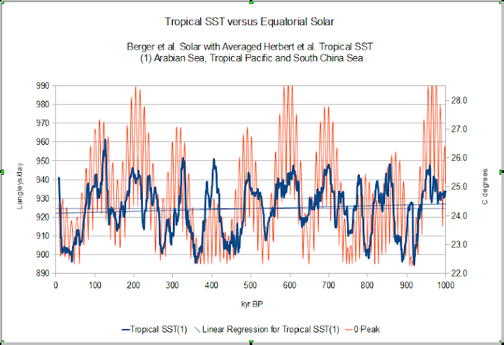
Yes and no. What you have at the equator is ~10ka peaks related to the precessional cycle that vary by about +/- 2ka. That can produce any multiple of 10ka +/- 2 ka. Precessional cycle is the big dog. Eccentricity would be a nudge. Instead of focusing on ice which is remarkably unstable, distorts the Earth’s crust, I focus on the tropical oceans. In fact, Herbert et al. 2010 has Arabian Sea, South China Sea and Tropical Pacific reconstructions that you can bin and average for a fair, tropical ocean reconstruction. The Atlantic reconstruction has some wicked gaps. That and the Berger solar for Equatorial peak insolation, match nearly perfectly for a million years.
The next strongest signal looks like 400kyr, but there is a weak ~100kyr in the mix.
captdallas2 0.8 +/- 0.2 January 25, 2015 at 3:43 pm Edit
I don’t find that at all. Here’s what I get:
I doubt yours, because nobody I’ve read thinks there is a 10 kyr cycle in the insolation data …
But I could be wrong. I just checked my figures, however, and I don’t see any error.
w.
Wilis, PEAK insolation. It is peak that can start melt, that reduces albedo that continues melt if you are looking at ice sheets. It is also Peak that would produce a maximum SST, (the rectifier and battery analogy). I just used latitude (maximum) instead of latitude June. With Eccentricity change you have more days summer or winter plus a little more insolation, so your peak month can slip around a little from what I have read.
Willis, They look like this,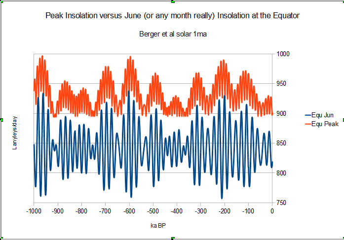
>>Captdallas
Can you make your graphs go the right way….
The trouble with this graph, is that insolation continues to peak, while the ice sheets are growing once more. That sounds counter-intuitive, and in need of further refinement and explanation.
R
ralfellis,
“The trouble with this graph, is that insolation continues to peak, while the ice sheets are growing once more. That sounds counter-intuitive, and in need of further refinement and explanation.”
That is pretty much how it works. The tropical oceans have a convective triggering temperature at around 27.5 to 28.5 C, then cloud cover and deep convection increases allowing more moisture to be transported to the poles to build the ice sheets. Clean ice sheets can survive pretty high insolation so they tend to grow more during higher solar insolation when they are likely to get regular clean snow accumulation. You do have critical insolation depending on how high the ice sheets are, where even clean snow can start to melt. Once you have some melt, the albedo drops and there is increased melt. So you have melt triggering energy and convective triggering temperatures providing two control points.
Ice sheets though are pretty finicky when they decide to collapse, so the orbital cycle doesn’t correlate as well with ice as it does with Tropical SST. So the chart with the Herbert et al. tropical SST versus orbital is the one I prefer to show.
It could have easily been more snow at 65N as less insolation.
=======================
Maslin and Ridgewell 2003 have an interesting take on the eccentricity problem:
http://sp.lyellcollection.org/content/247/1/19.short
Thanks for the reminder. I corresponded with Maslin when researching an Ice Age novel.