Guest Post by Willis Eschenbach
Well, either it’s a genetic defect or I’m just a glutton for punishment, but I’m going to delve some more into the ice ages. This is a followup to my previous post, Into and Out Of The Icebox. Let me start by looking at the cycles in the insolation and the cycles in the geological temperature. I’ll use the same temperature proxy dataset used in the discussion by Science of Doom here and here, which is the Huybers ∂18O dataset . For the insolation, I’m using the same Berger dataset that I used in my last post. Figure 1 shows the cycles in the two datasets:
 Figure 1. Periodogram of the Huybers temperature proxy dataset (blue) and the June insolation at 65°N from the Berger geological insolation dataset.
This graph demonstrates extremely clearly what is called the “100,000 year problem”. As you can see, the length of the ice ages has a very strong 100,000 year cycle, with a cycle amplitude greater than 40% of the swing of the data.
But in total contradiction to that, the June insolation at 65°N, which is the insolation that is supposed to cause the interruptions of the ice ages, has virtually no cycle strength in the 100,000 year (100 Kyr) range. The insolation has its greatest cycle strength between 19 and 24 Kya, and a smaller peak at 41 Kyr, but there is almost no power at all in the 100 Kya range.
It is worth noting that both the temperature and the insolation do show power in the ~ 23 Kyr and the ~ 41 Kyr range … but only the temperature has power in the 100 Kyr range.
Now, back in 2006 Gerald Roe wrote a paper called “In Defense of Milankovich”. In that paper, he said that the reason there was little relationship between the Northern Hemisphere insolation and the ice ages was that people were looking at the wrong thing. His point was that when the sun increases, the ice doesn’t immediately disappear. Instead, what changes is the rate of melting of the ice. This is also called the “first difference” of the ice volume. Roe used an earlier version of the same Huybers temperature proxy dataset I’m using to demonstrate his hypothesis, reasoning that the ice volume is a function of the global temperature.
So let’s start by looking at the effect of taking the first differences on the underlying cycles. Figure 2 is the same as Figure 1, except that I’m using first differences instead of using the raw Huybers temperature proxy data.
 Figure 2. Periodogram of the first difference of the Huybers temperature proxy dataset (blue) and the June insolation at 65°N from the Berger geological insolation dataset.
Now, that is an interesting result. As you might imagine, it hasn’t introduced any new frequencies into the mix. However, it has greatly decreased the size of the 100 Kyr cycle, slightly increased the size of the 23 Kyr cycle, and slightly decreased the size of the 41 Kyr cycle.
And what would be the result of those changes? Well, the correlation will indeed be better, as Roe observed … but for the wrong reasons. The correlation will be greater because in the temperature data (blue) the ~ 20 Kyr cycle and 41 Kyr cycles are now about the same size as the 100 Kyr cycle. So those cycles will fit better … but we still have no explanation for the 100 Kyr cycle.
In any case, here’s the match between the June insolation at 65°N and the first difference of the temperature proxy:
 Figure 3. A comparison of the June insolation at 65°N (red) and the first difference of the ∂18O temperature proxy. I am using the negative of the ∂18O data, so that increasing values show increasing temperatures.
Looks good, doesn’t it … but it’s not. Unfortunately, this is merely a wonderful example of the human propensity for seeing patterns. If you look at parts of this, it looks like a perfect match. The problem is, humans are shaped and bred by millions of years of evolution to find visual patterns … and as a result we find patterns even where no such patterns exist. The best example I can give you is that virtually every culture has found constellations in the stars. We identify Orion and Gemini and a host of others … and despite that, the stars contain no such patterns, just a random scatter.
And when we look closely at Figure 3, we can see that in many of the cases, the blue lines are in between the red lines … in all, they seem to be aligned at around 600 Kyr BP and also around the present, but badly out of alignment in between.
In order to keep ourselves from making such mistakes in pattern identification (among other reasons), we’ve invented an entire branch of mathematics called statistics. It allows us to do things like measure just how much of one variable is explained by another variable. The measure of this is called “R^2”. It varies from 0.0 (no relationship) to 1.0 (one variable totally explains the other).
And the R^2 value for the two variables above? How much of the first difference of the temperature variation is explained by the variation in northern insolation?
Well, the R^2 of the two is a mere 0.05 … that is to say, the June insolation at 65°N only explains about 5% of the variations in the first difference in temperature. Color me unimpressed.
Now, it’s possible that there is some lag in the data. To check that, we can run a “cross correlation”. This looks at the correlation, not just at the same time, but at a variety of time lags. Here is the cross correlation of the two variables:
 Figure 4. Cross correlation of insolation and first difference of temperature. Positive lags show temperature changes lagging insolation changes. Blue lines show the level where the p-vaule is 0.05, which must be exceeded to achieve statistical significance.
So … there you have it. The relationship just barely achieves statistical significance. Is it true that looking at the first difference of the temperature improves the correlation? Yes, it is … but for the wrong reason. Taking the first difference of the temperature proxy reduces the amplitude of the 100 Kyr signal and increases the amplitude of the ~20 Kyr signal. Since the ~ 20 Kyr signal is the largest signal in the insolation, as a result the overall correlation increases … but this still doesn’t help us at all with the “100,000 year problem”. Not only that, but at the end of the day, the relationship is so weak as to scarcely achieve statistical significance.
Me, I’d say that Roe certainly didn’t solve the 100,000 year problem … although as always, YMMV …
Best wishes to everyone,
w.
My usual request—if you disagree with someone, please QUOTE THEIR EXACT WORDS THAT YOU DISAGREE WITH. This is the only way for everyone to be clear as to the exact ideas that you are objecting to.
The most interesting dots for me were the temp and forcing at 2K years. [They] are quite large and are aligned, both in the original graph and the first differences.
It looks to me like you have found the explanation for the Minoan Warming, the Roman Warming, the Medieval Warming and the Modern Warming.
An interesting thought indeed …
w.
maybe there is a beat frequency between two orbital cycles with similar periods?
It appears that your original data may have been one temperature point every thousand years. This would make the 2K period the highest frequency with any mathematical content (the Nyquist frequency). Digitally sampled data contains all of the higher frequency power present in the unsampled signal, it just appears at the wrong frequency. Thus, it’s possible that the 2K peak is aliased from other frequencies, and not actually real data.
Am I missing something here? Don’t you need a 1K cycle, not 2K, for Minoan, Roman, etc warm periods?
My thoughts as well. However as I recall Bond events are something like 1500 +- 500 years. The interval is not always the same. Looking at the graph it seemed apparent that the resolution was limited to integer intervals, so it would be unlikely to reveal the jitter in Bond intervals. What also struck we was that the graph started at 1, not zero, so maybe it was accidentally offset by 1.
The important point for me was that I know of no orbital cycle that has power at 2k years. Since it is in the graph, I would like to know why it is there. Is it an artifact of processing, or is there truly an orbital cycles that has significant power at 2k years? Because if the result is real, then Willis truly has found the cause of Climate Change.
ferdberple – Thanks. Hopefully someone will take this further …..
Having a good understanding of the 2K year coincidence, since we should have more and newer evidence would seem to be critical.
As Tom points out, that is an artifact of the data being given with one point every thousand years. The 2K “signal” is an artifact. All that I an adding to Tom’s comment is that I looked at the file and confirmed his inference.
I´ve commented here before that centennial & millennial scale fluctuations in the climate of the Holocene & other interglacials appear to me to stem in large part from solar effects modulated by Milankovitch cycles in orbital & rotational mechanics.
IMO there really is no serious 100K problem. The switch from ~40K glacial cycles to ~100K could result from as simple as a change as more ice accumulating on the planet after the first 1.4 to 1.8 million years of the Pleistocene, resulting in a higher baseline albedo at the time of the Mid-Pleistocene Transition in glacial pattern. (BTW the recurring pattern is not an artifact of the human tendency to see patterns but an objective reality, as well shown in proxy data of all sorts.)
If not albedo then some other factor intrinsic to the climate system is liable to have flipped the switch, rather than some of the Deus ex Machina external phenomena hypothesized. Bear in mind that the shorter term Milankovitch periodicities still operate during the longer glacial cycles since the switch c. 1.2 million to 800K years ago. They have long been recognized as the stadials & interstadials within NH glaciations.
For example, the Wisconsin, the last glaciation, showed major stadials at about 40K year intervals, followed by the thousands of years long Last Glacial Maximum, during which arguably the planet entered a third stable mode (super glacial, to go with glacial & interglacial), during which the North Atlantic resembles the Arctic now. The LGM was framed by Heinrich Events, armadas of icebergs, the glacial equivalents to the Dryas Events during deglaciation.
Another point to consider is that 100K years is an average. The duration of glacials since the switch varies, as of course so too do interglacials. They are not all precisely 100 & 10 thousand years long. Far from it in the case of interglacials.
Further, while orbital inclination shows 100 Ka periodicity, eccentricity displays two periods at 95 & 125 Ka, which could combine to yield a 108 Ka effect.
http://www.sciencemag.org/content/277/5323/215
Eccentricity has been ignored in the past because it was thought not to have a big enough effect. However, the major component of variations in eccentricity occurs on a period of 413,000 years. As noted, other terms vary between components 95,000 & 125,000 years (with a beat period 400,000 years), thus loosely combining into a roughly 100,000-year cycle. This interests me because since the switch, ¨super interglacials¨ have been observed at about 400 Ka intervals. The Holocene might become one.
There is reason to be hopeful that the supposed 100 K problem will be subject to better analysis in the next few years, thanks to Antarctic ice core data from as far back as 1.5 million years ago, ie covering the period of the MPT:
http://www.sciencedaily.com/releases/2013/11/131105081228.htm
Study of the emerging data has already provided good evidence is support of the Milankovitch Theory:
http://www.nature.com/nature/journal/v448/n7156/full/nature06015.html
milodonharlani January 25, 2015 at 10:21 am
Yes, and it “could result” from the effect of gamma rays on man-in-the-moon marigolds … I fear that handwaving at albedo or “some other factor intrinsic to the climate system” doesn’t advance the discussion in the slightest. It “could result” from a lot of things, but without an actual physical explanation such speculation doesn’t help us.
So yes, there IS a 100,000 year problem. The ice ages occur very regularly, as shown by the periodogram in Figure 1. But why?
w.
There is no 100K problem for Milankovitch theory, since the prior 40Ka cycles continue during the longer glaciations of the latter Pleistocene.. Please address that fact. Besides albedo I also mentioned obliquity & eccentricity. That´s not handwaving. Detailed studies have shown how those parameters affect insolation. I cited some of them for your benefit. Again, you’d benefit from doing extensive literature searches before trying to reinvent the wheel. Nothing you´ve written on Milankovitch is in any way new.
milodonharlani January 25, 2015 at 1:52 pm Edit
Thanks, milodon. From Paleoceanography (emphasis mine):
Guess that lets us know you’re not in the “serious students” category …
And from Nature Geoscience 2013 (emphasis mine)
So yes, there is indeed a 100-kyr problem.
Near as I can tell, none of your three citations mentioned albedo, obliquity or eccentricity. One is Richard Muller’s hypothesis about dust due to the the inclination of the earth’s orbit. It’s interesting, but devoid of evidence, and it doesn’t explain why we come out of ice ages every 100-kyrs.
The other just says that the relationship between northern and southern hemispheric onsets of ice ages supports the Milankovich theory. Nothing about obliquity or eccentricity. The third just says they hope that the 100-kyr problem that you claim doesn’t exist will be solved in the future. Sorry … you’re still handwaving.
“Again”, as you say, if you can show me before and after periodograms of the Roe hypothesis done by someone else, or a cross-correlation analysis of the Roe hypothesis, you might have something. I don’t think you can. I’ve looked and I haven’t found them. I think you’re just throwing mud and hoping it will stick.
w.
The question that comes to mind is this: Is there a latitude at which the 100k year orbital forcings are aligned with insolation?
It could well be that the ice ages are more complicated that insolation at a single latitude. Maybe it is a non linear interaction involving the whole planet.
Huh? Which 100 Kyr orbital forcings are you talking about?
w.
sorry, wrote that in a hurry.
Is there any latitude or time of year at which the insolation does have significant cycle strength in the 100,000 year (100 Kyr) range?
I´d look at the Arctic, since that´s where major NH ice sheets originate, such as the Innuitian & even Laurentian sheets. IMO even 65 degrees N is a little too low. The Innuitian is based on Ellesmere Island, high in the Canadian Arctic. As all here know, the weight of the Laurentian accounts for Hudson Bay, but it too starts out at higher latitude before spreading south to gouge out the moraine that is Long Island (during its last advance in the Wisconsinian glaciation).
As Bill Illis has sagely commented, 75 N signifies more than 65.
ferdberple January 24, 2015 at 10:57 pm
No. Other than above the Arctic circle the time of year makes little difference. And the only difference due to latitude is the strength of the 41,000 year cycle, which increases steadily from zero at the equator to a maximum at the poles, where it is about equal in strength to the ~ 21,000 year cycles..
milodonharlani January 25, 2015 at 10:29 am
Thanks, Milodon. It makes little difference whether you look at 65°N, 75°N, or 90°N—there is still no 100,000 year cycle in the insolation data.
w.
That some don´t detect a 100Ka signal in insolation isn´t a problem for Milankovitch theory, as I´ve noted. It just means that, for these researchers, some other mechanism must explain the switch to longer cycles, which still, as noted, contain the prior insolation driven shorter cycles.
You might not like this 2013 study, since its authors tested their hypothesis with a model, but it makes sense:
http://www.nature.com/nature/journal/v500/n7461/full/nature12374.html
The mathematicians and statisticians looking at the problem haven’t integrated lag temperature effects of continental scale ice build-up, which itself creates its own climate and changes earth temperature, largely due to changes in albedo, but also changes in ocean currents and heat distribution from the equator to the poles. These lag effects are of the order of several tens of thousands of years.
There is no linear relationship with earth temperatures and incoming insolation.
Thingadonta, that’s exactly what the cross-correlation analysis does. It looks to see if there are lagged effects.
w.
I noticed on the previous article the insolation shows repeated stronger cycles which happens to correlate with the onset of decreasing temperatures.
I’m thinking this is potentially evidence of a strong negative feedback mechanism where warming eventually results in a strong negative feedback in some cases, but not in others.
It may lead to something insightful (or, it may lead to a mess) but you can take the FT of your cross correlation, divide it by the power spectrum of the input, and inverse FT to get an impulse response (this is Wiener deconvolution).
It may lead to a recognizable type response, for which Roe’s derivative relationship is merely a first order approximation. The impulse response so derived is lousy after some time interval, so you need to choose some point at which to taper it off with some window function. Then, you can FT that to get a smoothed frequency response.
Are we asking the right questions?
1. What causes the Ice Ages?
or,
2. What causes the termination?
I like #2.
Glaciation and 8º to 10º C colder than present seems to be the normal state of Earth’s climate for the last 3 My.
— I envision the glacial terminations as a bifurcation in a non-linear system response. Not predictable, but statistically inevitable, once insolation extremes force the system to a new Lorentzian attractor. The descent to (return to) glaciation is an order of magnitude slower (50 Ky vs 5 Ky for termination). That I realize is just a fanciful Gedankenexperiment, absent of real world data, since no one can build a climate simulation to simulate something that isn’t calculable.
asking the right questions …yes…
climate earth system is very complicated, and nobody understand it but still want to find simple explanations.
Do you know anything at all about chaotic nonlinear oscillators and attractors? Any basis on which to call it a simple or complex explanation?
I too like #2 but look at it from a physical point of view. At the termination point it has achieved its maximum covering of ice, snow and permafrost, latitude 35 to 40 Northern hemisphere. A small onset of extra warming and changes in the existing climate pattern will have an effect on the large area at the lower latitudes, change the albedo and release of methane from the permafrost subsequently followed by a further temperature rise.
2. What causes the termination?
The ice weight?
I agree with joelobryan that the glacial-interglacial system looks like a weakly forced nonlinear oscillator.
giving it some time to ponder, it seems to me Willis IS indeed asking #2. But the dataset he uses, the MC wiggles, addresses #1.
As Dr. Scienceofdoom lays out, the precession of the equinoxes and obliquity alter distribution across the globe. But eccentricity does change global TSI. And when high obliquity aligns with summer65N insolation aligns with a high eccentric perihelion, any sort of nonlinear changes to a massive NH ice sheet can be sudden, unpredictable, but statistically inevitable.
The descent is a process of evaporation, 600 kcal/kg, followed by snow/rain and ice formation, 100 meter of lower sealevel.
The upswing in temperature is purely melting, 80 kcal/kg.
The descent requires substantial more energy and might explain the slower slope.
Willis , I don’t do this kind of thing too often, but a derivative of the time domain function, when Fourier transformed, should yield some proportionality constant times frequency times the frequency domain function. The Figure 2 spectrum plots against the wavelength rather than the frequency, but It seems to me that with a bit of time domain smoothing (to take out the high frequency peak at 2000 years), and an optimally chosen proportionality factor, it ought to be possible to get a much better looking fit for Figure 2. I.e., the 100K peak should be almost completely suppressed for an appropriately chosen proportionality constant.
‘Fraid you’ve lost me there, TYoke. Why would you want to invent some transform that would suppress the peak? What am I missing here?
w.
The point of taking the time derivative of the ice volume is the hope that the new curve will better match the Milankovitch cycles, but to get agreement the 100k peak needs to be a lot smaller (suppressed).
If a time domain curve is Fourier Transformed and then plotted, not as a function of frequency, but instead as a function of wavelength, then it is called a periodogram.
Fourier transform theory says that if the time derivative of a function is transformed, it goes over in the other domain to the transform of the original function multiplied by frequency. Therefore, if the derivative curve is plotted as a transform (periodogram) we should see the original periodogram multiplied by frequency. Since the RHS of the wavelength plotted graph corresponds low frequency, peaks on the RHS of the derivative graph ought to be HIGHLY suppressed. I.e., no 100k peak. Your periodogram showed a significant 100k peak in Figure 2, and I’m trying to figure out why.
There should be no peak there since Figure 1 should simply be multiplied by frequency to get figure 2 and frequency on the RHS goes to zero in a wavelength plot. Likewise, the 2k peak, which is on the LHS in Figure 2 ought to be very large since the frequency is large. The 2k peak is instead approximately the same size as for Figure 1 and I don’t understand that either.
The only thing I could think of to explain the lack of expected difference between Figure ! and Figure 2 is that Figure 2 was plotted with a very small proportionality constant plus a y-offset of some kind. Another possibility is a discretization artifact of some kind.
I was looking at Figure 2 again, and actually for the most part the blue line in Figure 2 does look like the blue line in Figure 1 multiplied by frequency(where frequency has units of say 1 cycle/30k). The exception, and the thing that threw me off, was the lack of change in the 2k peak. Fourier theory says, for continuous logic at least, that that peak ought to be MUCH larger in Figure 2 than it is in Figure 1. Presumably the lack of change is a discretization artifact.
What about the possibility that the celestial geometry associated with Milankovich is not the driver of the ice ages as everybody (including me) has been taught?
Milankovich’s theory is a version of cosmo-climatology. Svensmark’s cosmo-climatology is another version based on climate modulation from interaction among Earth, Solar and stellar systems.
Is there any basis for regarding the climatic effects of galactic cosmic rays to be quasi-periodic on the same time scales as the Milankovich cycles? Is this idea even worth considering?
It is worth considering but very hard work out. We may get bursts from the galactic core periodically but might not. We might also get them from other random sources. Very fun to think about until your head hurts with all the possible variations 🙂
There are two things that strike me about glacial episodes. One is that 100k years is a damned big time constant for most earth based systems. The other is that there is periodicity at all, and of such a shape.
Ice ages appear to end far more rapidly than they begin.
I cant explain either. Milankovitch appears to be inadequate as seen here. I LIKE Svensmark, but I can’t find any galactic 100ky periodicity there either.
Astrologers see ages in terms of solar system alignments which repeat at millienial sorts of time scales. But 100k years?
The form of the ice age time/temperature looks like short bursts (10-20ky) of intense warming followed by slow relapse into cold, with the usual heavy ‘noise’ in between.
Off hand I’d say that lack of cloud could cause it, but what would cause lack of cloud?
And yet ‘ve read reports of investigations using paleo-botanical markers in ancient soils and lake sediment that indicate the switch to an ice epoch temperature regime could be as swift as 9 months! That’s almost catastrophic in speed.
Not a math person, but did Mr. Eschenbach just repudiate Milankovich cycles currently applied to geological temperature or just having to do with 100 yr. cycle?
Bravo. Milankovitch is a layer, one of many, and capable of being completely overwhelmed by many other layers either individually or in concert. The 400 year eccentricity cycle has the greatest theoretical effect but has no power in the Pleistocene (which we still live in).
Please find the following from none other than Richard Muller:
http://muller.lbl.gov/papers/nature.html
Plankton are very responsive to insolation. Just look at the COGO map showing the ocean response following the ITCZ. This led to the deep sea cores and Dr. Shackleton over ascribing Milankovitch to climate in general.
Layers and layers. The very same deep sea cores show a pretty abrupt transition from something like a 41kyr obliquity cycle to something like a 100kyr eccentricity cycle between MIS 36 and 22 about a million years ago.
Layers permutate. Any apparent oscillation can result from the net effects of many different layer influences.
Richard Lindzen wrote a paper in the 90’s about the remarkable fact that Tropical freeze lines during the Last Ice Age were about 1 kilometer lower than during the Holocene, even while Specmap showed tropical ocean temps to be about the same as today. His solution to the problem was a steepened tropical lapse rate, as would be expected, and in order for this to work a reduction in TSI of 3.1% to 4.6% which is better than the M-cycle numbers. Nevertheless the cause implied in that paper would be the sun itself – but how? Since we are again bereft of an answer of how TSI might wary that much.
TSI does not vary that much, but the amount of solar radiation that makes it to the surface of the Earth can vary within that range as the result of changes in the Earth’s albedo due to cloud cover, snow and ice.
Also, I think part of the problem here is looking for a single mechanism as the answer, i.e. it is either the M-cycles OR clouds, snow/albedo OR plate tectonics/ocean currents OR a change in the composition of the atmosphere, etc.
So far, no single mechanism can explain the repeating patterns of the ice ages (41K years shifting to 100K years). While we are at it, a good explanation should also cover the causes of long term hot house vs. ice house climates, not just glacial vs. inter-glacial variations within our current ice house epoch.
Unfortunately, just our luck in reality it is probably a combination of most of them – cycles within cycles, each with differing periodicity, producing commingled patterns of constructive or destructive interference. A dynamically chaotic mess with no simple answers. Go figure.
How much long term data do we have on TSI?….none.
100 years is not long term nor even is1,000 years, in the context of natural history.
Per rgbatduke January 23, 2015 at 6:50 am concerning Dark Matter:
“A clump of DM falling into the sun (or a locally thicker patch of DM falling into the sun, or the earth) would have extremely odd effects.”
Perhaps also affecting those nasty asteroid falls:
http://www.dailygalaxy.com/my_weblog/2014/05/our-solar-system-orbit-through-milky-ways-dark-matter-disk-does-it-trigger-comet-impacts-and-mass-ex.html
I don’t think we need exotic DM theories, but we do need to consider the fact that our local star may vary far beyond anything that we have witnessed or studied. I know that is heresy, but the rapid temperature changes during Ice Ages with DO and H events beg for some driver that operates very quickly.
Perhaps Robert Ehrlich’s theory of solar resonant diffusion waves has merit, but how could we even study them, unless there is some terrestrial imprint that we could find, or look for.
I forgot the reference to Ehrlich’s paper which is here: http://arxiv.org/abs/astro-ph/0701117
I also thought that there was a WUWT article on this very topic a few years back.
Mohr is on the right track. TSI should be considered. We have a proxy for that that works nicely…ICE
And there is paleo SST as well.
Trying to squeeze an ice age out of changes in NH insolation does not work.
mpainter – you are correct. Ice is an excellent proxy. I am kicking myself because I once came across a paper that looked back, via palynology, and chironomid midge data, at the climate of the Pacific NW during the last 50,000 years.
I can’t find the pdf but the standout feature was the wild gyrations in climate that occurred during this time. The last Ice Age was no longer a uniform cold period where everything was buried under two miles of ice, but was a wild inhospitable place, with mind boggling temperature swings, even though there were also times where temperatures approached todays even though winters were much colder. Also of note was the idea that ice advances were not uniform and the PNW probably wasn’t completely buried until the LGM.
Even at the LGM the PNW wasn´t completely buried by ice. In southern Washington & Idaho, plus Oregon there were more extensive montane glaciers, but no ice sheets.
” humans are shaped and bred by millions of years of evolution to find visual patterns”
They are shaped and bred by 200-300.000 years of evolution, and if you wanna accept most recent findings off the bat, then maybe as early as 500K, or up to 700K years, but really less for all we know. And then we still don’t know when they started being shaped for pattern recognition, which is safe to assume a lot less still.
200-300K years is the best Dawkins would ever grant you in any of his talks and discussions – for human evolution, not pattern recognition.
Long before apes could walk upright animals were migrating because of seasonal cycles and running away from odor patterns and ripple patterns in long grass . Animals can recognize patterns and cycles but They don’t do the “why” bit that humans do , They just react .
Matt January 24, 2015 at 11:13 pm
Which is why I was quite careful to say “evolution” and not “human evolution” … not my first rodeo, my friend, and I know that I’ll be fact-checked to the max, so I take great care with what I say.
Now if folks would only take the same amount of care with their reading …
w.
The naming of constellations is not the assumption of a pattern in how stars are distributed in space but how the dots of light in the sky do not vary much from night to night. Orion’s belt didn’t look like a belt to cultures unfamiliar with Orion but they all saw the same three stars reliably reappearing each evening and moving across the sky as they had done before.
As for evolution; the oldest fossils are 3 billion years old, so why have only millions of years of evolution led to the human propensity for pattern recognition? Of course, “millions” does not exclude “billions” but…
And humans may have been “shaped” by “millions” of years of “evolution” but I’d like to see how they were “bred” by evolution. I did try to be careful with my reading.
There is another thing that bothers me about these types of analyses. It assumes a perfectly round and perfectly flat Earth. At sea level the instantaneous insolation is about 1000 watts/m2. At 6,000 feet that number is closer to 1175 watts/m2 and at 10,000 feet is closer to about 1250 watts/m2. The northern hemisphere at higher latitudes is at a much higher altitude than the southern hemisphere at the same latitude.
Also, coupled to this is that in Eurasia at the same latitude the altitude is much lower than in North America. If you look at the ice sheets, they are far thicker in North America than at the same latitude in Siberia.
It is as simple as looking at snow cover, which lingers far longer at the higher altitudes in North America.
Your simplistic (not just yours) use of the standard averaged out insolation values fails to capture these very significant variables.
Willis,
I seem to be a pattern recognition evolution victim.
In this graph from you last ice box post
I see the earth in a glacial state when swings in insolation are at a minimum, and the glacial state ending when insolation swings increase to a larger magnitude.
Clearly a false non statistical patter recognition based observation.
There’s also the fall in sea level(around 300feet???).
What would this mean to the decline in temperature with altitude?
The several kilometres of glacial ice presumably makes a difference???
Maximum lowering was about 140 meters.
denniswingo wrote: “At sea level the instantaneous insolation is about 1000 watts/m2. At 6,000 feet that number is closer to 1175 watts/m2 and at 10,000 feet is closer to about 1250 watts/m2.”
Can you provide a source for those numbers? I find them hard to believe. I think that most of the difference between the top of atmosphere insolation of 1360 W/m^2 and 1000 at the surface is due to absorption by O2 and O3 in the stratosphere.
My direct measurements of the output of solar arrays in my business. We have a mobile system that we take around and do measurements for solar array output at specific sites. I have built satellites and directly measured the solar array outputs in space.
We did a one year study at the Tehachapi wind park at 4,000 ft altitude and at Yellowstone national park both at 6,000 feet and at 8,700 feet and at Mammoth at 9,500 feet altitude. Also, Mountain View Wyoming at about 5,000 feet.
As for Oxygen, it mostly absorbs at near UV wavelengths. The decrease in insolation between space and sea level is mostly scattering, reflection, and water vapor.
Also, NASA JPL provides solar cell calibrations for space applications and they use a high altitude balloon for the purpose. They get space level insolation at +100,000 feet.
Reference for Spectral absorption by Oxygen.
http://onlinelibrary.wiley.com/store/10.1029/98JD02799/asset/jgrd6210.pdf;jsessionid=C20831FC9570FAF8A086251447387656.f04t04?v=1&t=i5cwa94o&s=f0089494c0470503fba6666c7f50f7c6f0f61386
References for JPL space calibration of solar cells.
http://arc.aiaa.org/doi/abs/10.2514/3.28191?journalCode=jsr
http://trs-new.jpl.nasa.gov/dspace/bitstream/2014/7428/1/03-1288.pdf
denniswingo,
I remain skeptical. About half the atmosphere, and almost all the ozone, is above 5 km, so at km insolation should be much closer to the surface value than to the top-of-atmosphere value.
There is no point to look for correlation between insolation changes and temperature changes. If anything, temperature changes (driven by area under ice) depend on insolation (not its change). But I suspect the main reason why you lost so much of that 100k cycle in the differences is because of how your periodogram is calculated. In the temperature changes graph, you get series of peaks from times when the Earth is unglaciating, and low absolute values while the Earth is reglaciating. That’s because the system response to insolation is nonlinear and stateful.
Evaluation of correlation coefficient (r2) is only skillful for linear or near-linear responses. When the response is nonlinear, much more can be read from a scatterplot than from evaluating r2. There are many cases when scatterplot reveals clear dependency of the two variables while the r2 value is 0.
Absolutely. The Internet is littered with warnings about improper use of r2. It assumes the relationship is linear. It reminds me of the old saying that it’s impossible to prove a negative. A high r2 value does indicate high correlation. But a low r2 does not necessarily indicate low correlation, it simply says that either the correlation is low or the correlation is non-linear and too complex for r2 to capture.
Chris
denniswingo January 24, 2015 at 11:36 pm Edit
Say what? It assumes nothing of the sort. The fact that I didn’t mention an atmosphere doesn’t mean that I assume there is no atmosphere, and the fact that I didn’t mention mountains doesn’t mean I assume a flat earth.
As to your claim that “in Eurasia at the same latitude the altitude is much lower than in North America”, the east half of North America is about the same elevation as much of Eurasia, while the western half of North America is higher … so what? Does that somehow solve the 100,000 year problem?
w.
The Laurentide ice-sheet over Hudson Bay was about 3000 metres high (even relative to today’s sea level, it would have been over 3000 metres). Thus, there is now a lapse rate to consider and even higher solar radiance as denniswingo noted as well as gravity pushing the ice downhill from a central spreading region .
http://img.gawkerassets.com/img/18qtm8pbrer6npng/ku-xlarge.png
This map is from Arthur S. Dyke 2002
https://notendur.hi.is//~oi/AG-326%202006%20readings/Canadian%20Arctic/Dyke_QSR2002.pdf
Dyke 2004 also has a detailed outline of the deglaciation process in which Hudson Bay still had large-sized glaciers lasting until about 7,600 years ago.
https://www.lakeheadu.ca/sites/default/files/uploads/53/outlines/2014-15/NECU5311/Dyke_2004_DeglaciationOutline.pdf
This ^^^^
Summit Camp in Greenland is 3200m above sea level, so it seems reasonable to assume that the surface of the Laurentide Ice Sheet at similar elevations (most of Canada) would have “enjoyed” similar conditions during the last glaciation.
While that does little to explain WHY the ice accumulated and melted when it did, it does strongly imply that both processes would have strong feedbacks associated with them, with the surface of the ice sheet growing progressively colder while the ice accumulated, and progressively milder while it melted, merely on the basis of the changes in elevation.
Let’s say the 3000 metre high glacier over Hudson Bay, 2000 kms from the ice-sheet front took 10,000 years to melt back to zero.
That is 0.3 metres (1 foot) per year of melt per year and 200 metres in distance of the ice-front melting back per year.
That is a pretty slow process.
Can you imagine if we were time shifted 20,000 years to the left such that the Larentide ice sheet was the present. GreenPeace, McKibben,Gore, et al would be warning of a loss of ice and catastrophic warming……. oh wait.
But I doubt our Canadian friends would mind Ms. Larentide getting lost though.
Willis
You are relying on models for solar insolation that take out all of the variability, specifically variability based on altitude. Your insolation number does assume sea level insolation. At no point did I say no atmosphere. Quit being defensive and listen.
And yes, it does solve the 100,000 year problem. The reason that this has not been solved is that the research community, including you, use simplified models. This is EXACTLY what the AGW community does.
The 100,000 year problem is based on the eccentricity variable. How about doing some research on what the difference in insolation is at minimum eccentricity and then at maximum eccentricity, and then use altitude corrected ground insolation numbers.
These are subtle changes, yet obviously OBSERVATIONS show that we are in the 100,000 year cycle and have been for the last 800,000 years. Before that the cycle was 41,000 years, which is the obliquity cycle.
If OBSERVATION shows one thing and your model says another, guess which one is wrong.
The vast, mountainous ice sheets also had a dramatic effect on other meteorological phenomena, such as wind circulation. Compare what weather would be like on Antarctica without its ice sheets.
denniswingo January 25, 2015 at 1:10 pm
I’m sorry, but I truly don’t understand how including mountains somehow solves the 100-kyr problem. You wave your hands and say I should be doing “some research on what the difference in insolation is at minimum eccentricity and then at maximum eccentricity, and then use altitude corrected ground insolation numbers.” … sorry, how about YOU do that and come back and show us your data and code. That’s your hypothesis, so it’s yours to support, not mine.
Say what? Sounds like you don’t understand that the 100-kyr problem is exactly that the Milankovich model can’t explain the 100-kyr cycles of the ice ages.
w.
“The 100,000 year problem is based on the eccentricity variable. How about doing some research on what the difference in insolation is at minimum eccentricity and then at maximum eccentricity, and then use altitude corrected ground insolation numbers. ”
What would be the rules for eccentricity
Does the orbit have keep a 365 day period.
And could be something like orbit near Venus and Mars.
Or does the time of the orbit change- more or less than 365 day.
If so how much less or more does the duration of orbit have?
Or Earth orbit is Perihelion: 147.1 million and
Aphelion 152.1 million
So make more circular and less than 365 day to would be a
147.1 by 147.1 orbit.
Or for longer year: 152.1 by 152.1 million orbit
Starting premise seems to me that if earth were completely covered
by ocean and say it kept a 365 year it should little effect.
Or would it actually be warmer or cooler depending upon whether had least eccentricity
or greatest?
Now the greater the eccentricity and the maintaining same length year, means
a longer time of the year furthest from the Sun, but this balanced against being significantly
closer and having a intense sun, though for much shorter portion of year.
Anyhow, it seems just less or more eccentricity isn’t enough info.
This print resolution image shows one cross-section of the age of the Greenland Ice Sheet as determined by MacGregor et al. (See citation under the “More Details…” button below) Layers determined to be from the Holocene period, formed during the past 11.7 thousand years, are shown in Green. Age layers accumulated during the last ice age, from 11.7 to 115 thousand years ago are shown in blue. Age layers from the Eemian period, more than 115 thousand years old are shown in red. Regions of unknown age are filled with a flat gray colour.
http://svs.gsfc.nasa.gov/vis/a000000/a004200/a004249/GIS_periods.06429_print.jpg
http://svs.gsfc.nasa.gov/cgi-bin/details.cgi?aid=4249
What a cool picture! Take home message: there is a hell of a lot more ice now than what survived the last interglacial.
I believe that is deceptive. The video made the point that the ice flowed under pressure. There is no way of measuring the effect of such movement on the deeper ice and the deeper, the more the problem. What we see in the deeper ice is residue, IMHO.
Have not yet figured out why but this gsfc image is completely contradicted by the GISP2 and NEEM ice cores. At NEEM, the ice level at the Eemian peak melting was only 400 meters below the present surface, and the total depth to bedrock was about 2530 meters if I recall correctly. No way was half the ice sheet deposited during the Holocene rather than preceding glacial intervals. Defies common sense.
Thanks, ren.
NASA Data Peers into Greenland’s Ice Sheet, at
http://www.nasa.gov/content/goddard/nasa-data-peers-into-greenlands-ice-sheet/
Is very interesting, showing that the Holocene produced a big part of the Greenland ice now in existence.
I’m guessing that the bottom ice could be wasting outwards under pressure all the time? Brett
I think joelobryan January 24, 2015 at 10:05 pm is on to something. Is there a way to massage the data to make the onset of a warm period distinct from the entry into a cold era?
Willis,
You write: “The insolation has its greatest cycle strength between 19 and 24 Kya, and a smaller peak at 41 Kyr, but there is almost no power at all in the 100 Kya range.”
What about 5*19 and 4*24 being close to 100? Could these cycles together with a couple of (maybe yet unknown) cyclic effects get amplified every 100ky by coincidence?
I found this article by Willis, probably a few days after everyone has stopped reading and commenting.
I did notice that Gerard Roe mentioned in passing at the end of his paper that the causes of the terminations was unknown:
“The Milankovitch hypothesis as formulated here does not explain the large rapid deglaciations that occurred at the end of some of the ice age cycles.”
I.e., the most important bit.
In Ghosts of Climates Past – Eighteen – “Probably Nonlinearity” of Unknown Origin I break the Milankovitch “theory” (actually family of theories) into two parts:
– The waxing and waning of the ice sheets on 20,000 yr and 40,000 yr periods – nicely explained by the high latitude insolation changes
– The terminations on 100,000 yr periods, not explained at all by any reasonable theory. In fact, the last few ice age terminations have taken place at something like:
I-II = 124 kyrs
II-III = 111
III-IV = 86
IV-V = 79
V-VI = 102
an average of 100,000 yrs but not actually on 100,000 yrs.
All very interesting.
Exactly, there is no 100 Kyr temperature cycle. It is n*41Kyr, for instance 80-40-80. LP-filtered that will become 100-100.
My two cents worth….
Once every 100,000 years (or so*) the precession cycle has summer solstice of the northern hemisphere (NH) at “perihelion” (the planet’s closest approach to the sun) when the orbit is at maximum eccentricity and the planet’s axial tilt maxed out at 24.5˚ in relation to the orbital plane. As conditions approach this maximum, exposure to the sun’s rays (insolation) at 65N increases causing the great northern ice sheets to melt away putting the Earth into an interglacial warm period.
*As the orbital mechanics (precession, obliquity and eccentricity) oscillate distinct to each other the 100 thousand year occurance for this “peak” (IMHO) varies (using SoD’s numbers) from 80 to 120 thousand years. To a lesser degree this would also be true for the maximum tilt position.
Obviously there are other factors that affect the intensity of the “peak” orbital position. Is there a name for this “peak” event?
wobble? Rotational wobble. Increased weight has to destabilize the rotation.(throwing a top will show and a few other interesting things) Currently the earth is moving about one day a year from the perihelion in the NH from sometime in the 1970’s. (the ancient Wei calendar has a ~400 yr. cycle, with another cycle described in days , something that equates to 59 or 60 years, I think it was 21,800 days) One thing I am curious about is why no one is showing or thinking about fractals, or about Fibonacci numbers. Ice ages are repeating time frames with smaller events happening in between. One thing that does bother me is that everyone seems to only graph just this idea or that. Other variables can or would cancel out sometimes and add at others. They aren’t random numbers. The past ice ages weren’t 150 K yr. nor were they 75 K yr. There are upper and lower limits. ….. It is my opinion that somebody does know. If I’m thinking it somebody else is too. and has it already figured out… knowing when it will turn colder is a bigger secret than when it will turn warm.. in fact the psychology of telling people that it is warm when it is not, tells you something…
Rishrac, thanks for the reply. Sorry for the delay, you made me think. First, you exposed the huge error in my post. I meant to say minimum as opposed to maximum, when I said “the orbit is at maximum eccentricity”. The corrected part of my post should have read thus…
…“Once every 100,000 years (or so*) the precession cycle has summer solstice of the northern hemisphere (NH) at “perihelion” (the planet’s closest approach to the sun) when the orbit is at minimum eccentricity and the obliquity cycle has the planet’s axial tilt maxed out at 24.5˚ in relation to the orbital plane. As conditions approach this orbital combination, exposure to the sun’s rays (insolation) at 65N increases, the great northern ice sheets retreat and the Earth returns to another interglacial warm period”
I left the error unchecked to see if anyone would call me on it. Not unreasonable considering this portion of the thread belongs to Scienceofdoom.
Willis’s post searches what is known for the transition from the 41Kyr glacial period to the 100Kyr glacial period some 400K years ago. The answer, just like AGW’s magnitude, remains highly uncertain. We all love Willis’s posts.
I’m no scientist but my parents were. So I’m going to hazard a guess….something changed. I think it may have to do with eccentricity. The orbit, although eccentric, went more eccentric thus changing the intensity of the precession/obliquity combination where the precession cycle has NH summer solstice at perihelion when the obliquity cycle has the planet’s axial tilt maxed out at 24.5˚ in relation to the orbital plane. So eccentricity could be a “nudge” (h/t captndallas) where every fourth (or fifth) combo we have a “peak”
Now (not assuming I’m right), the question remains…what changed the cycle? I think RGBrown of Duke hit the nail on the void in hinting about dark matter. Some sort of cosmic tug.
Rishrac, I do like your idea of people beyond our reach (suffering from mathematical certainty) who are in “the know”. I agree, better to preach the warming scare vs. the cooling scare.
All very interesting.
Oops, memory does not serve…I should have said “Willis’s post searches what is known for the transition from the 41Kyr glacial period to the 100Kyr glacial period over 1 million years ago” (instead of 400k years ago)
What I’m trying to describe is… not precession, it’s one pole or the other, at the same 23 ~ 24 deg angle as it revolves around the sun pointed away when it should be summer. No matter how many times I’ve thrown a top, that feature comes out. It will in the beginning revolve around a central point just like the earth does now. Then it will still revolve (and rotate of course) and the angle will be the same, but the ‘northern half’ of the top will point away from the point all the way around. A wobble stabilized. It would be interesting to know how much the wobble has increased or decreased since Columbus first noticed it. If you take a cup with a rounded bottom and roll it around a central point with an angle, it will do the same. You have to turn the cup in to get what the earth is doing now. You have to do a small secondary loop to get the top half to point inward to keep it rotating. In fact, I find it rather difficult. Physically the pattern that the earth is in may not be normal. Or it might be flipping between the 2 every so often. ( of course you could also revolve it around with the top portion pointing in)
Science of Doom, “All very interesting”,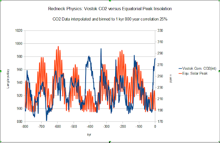
The electric company where I live does not [provide] DC voltage but with a bridge rectifier and a battery I can fix that. Not all that interesting but useful. Using 65N or 60N gives you the equivalent of a stray voltage that can create interesting patterns but with a sphere you would want to use the average applied voltage and peaks to figure out how to design your system.
At the Equator, you have a signal that is rectified with respect to either pole, so instead of a ~20ka cycle you have a doubled 10ka cycle. With that base you can get some neat transients. Add the oceans for a filter and you can get rid of a lot of the transients.
So just on the precessional cycle you can expect multiples of 10ka +/- about 2Ka which would be your strongest frequencies. When you combine that with the other orbital frequencies you get something like this.
Oh, that would be Berger solar and Vostok CO2 both archived at NCDC
captdallas,
nice work. the frequencies align. But the amplitude envelope cycles in and out of 100Ka phase withe VostokCO2.
Joel, “But the amplitude envelope cycles in and out of 100Ka phase withe VostokCO2.”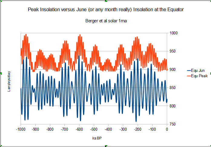
Here is a different look.
With a water world you would be looking for critical energy levels related to water to start an abrupt change. For biological you would be looking for “ideal” ranges and critical levels. CO2 would be related to both, SST and biological “ideal”. Abrupt de-glaciation would trigger a biological “ideal” where the glaciers retreat and in the oceans close to the melt water with that surge of nutrients.
So if you look at the chart above, you have a nice neat rectified envelope but below you have spikes not centered on the envelope peak. These power surges would not be obvious in a nice smoothed “average” insolation for any particular month. “Averages” have limitations.
Correlation does not imply causation. However, lack of correlation does refute a causal link, as in this post. TY for the Roe catch. Read the article yesterday. Obviously not carefully enough.
Good observation. So convenient to talk about 100 k cycles & no one really looks closely at the data. Thus science stumbles along.
Another representation, from
Bintanja, R. and R.S.W. van de Wal. 2011.
Global 3Ma Temperature, Sea Level, and Ice Volume Reconstructions.
IGBP PAGES/World Data Center for Paleoclimatology Data Contribution Series # 2011-119.
NOAA/NCDC Paleoclimatology Program, Boulder CO, USA
Over 3 million years:
http://climate.mr-int.ch/images/graphs/ice_level_3myr.png
Zoom over past 150’000 years
http://climate.mr-int.ch/images/graphs/ice_level_150kyr.png
With the corresponding temperature reconstruction:
http://climate.mr-int.ch/images/graphs/t_reconstruction-150kyr.png
Of course, ice forming or melting has to follow thermal changes, and it takes a long time to transfer so much energy.
When we split hair about tenths of degrees, we forget the thermal changes that are linked to such change of phase (water latent heat of fusion 334 kJ/kg)
At the current rate of melting, it may take 10’000 years for Greenland to have lost all its ice sheet, and 380’000 years for Antarctica. Until then, other cycles will have developed.
Urgency is a relative feeling.
Wondering why they are so interested in Eurasian ice. Eurasia never developed significant ice sheets. Why not use western North American ice, an area which likewise never developed significant ice sheets?
Ice sheets of Eurasia and North America are given. Both had a considerable ice amount.
from Wikipedia:
http://fr.wikipedia.org/wiki/Derni%C3%A8re_p%C3%A9riode_glaciaire#mediaviewer/File:Northern_icesheet-fr.png
There were substantial ice sheets in Eurasia, to include the British, Scandinavian, Alpine, Barents Sea, Siberian & Tibetan, some of which might however be considered montane glacier systems more than sheets. Plus systems as in the Pyrenee, Caucasus & other mountain ranges..
Once you get divergence from the presumed correlation any explanations just become speculation. I thought you guys at least would be cognisant of that after Al Gore and CO2
Willis, I have been at a presentation of Richard Lindzen in Brussels last year, who showed that for melting the ice sheets as happened during the warming towards an interglacial, you need not less than 200 W/m2 extra heat/insolation. The increase of CO2 and its increase in feedback of a few W/m2 seems not of much help in such periods. But where the 200 W/m2 comes from is still unknown. The most probable candidate is changes in cloud cover, but these are minimal during an ice age (minimum humidity) and increase with higher temperatures…
Still a lot of questions in this “Settled Science”…
It is my feeling that you cannot explain the Pleistocene climate shifts without big shifts in insolation values. But if you try to explain it all solely in terms of NH insolation, you will miss by a mile.
I should finish the the thought:
The ice age was _worldwide_ , from the tropics to the poles. Snowpacks on tropical mountains were thousands of feet lower than today. There were lower temperatures _worldwide_. Insolation changes in the NH cannot account for the _worldwide_ aspect ofthe ice age. When the Holocene began, temperatures increased precipitously _worldwide_. Most significantly, in my view, SST increased _worldwide_.
I have yet to see an explanation of the ice age which explains the worldwide increase in insolation at the beginning of the Holocene, which must have been.
Willis, I found your ‘icebox’ series extremely interesting, and I stand back in awe at your data presentation, thanks very much.
Being an ‘averagely evolved pattern spotter’, by your exposition, I would say that your Milankovitch based insolation changes versus paleo temperature plots would appear to suggest (1) that not every insolation swing correlates with a major temperature swing, but (2) pretty well all of the major temperature increase swings are associated with an upward insolation swing. This suggests to me that SOME of the insolation swings trigger the switch from glacial condition to interglacial condition.
Not, I hasten to add an original observation of mine, but one I first noted in John Kerr’s treatise, the Inconvenient Skeptic.
And I also like Fred Berple’s post picking up the 2kA cyclical blips that help with the Minoan, Roman, Medieval and current warm periods.
Imarcus.
Dear Willis,
Look at the wave equation and gain an understanding of oscillations. A pendulum (the ice age cycle) will react to a perturbation depending on where it is in its swing. A warm earth is hard to heat up. A cool earth is hard to cool down. The Milankovich swings depend on the current heat state of the earth when they occur. Milankovitch is an important but not sole factor in the earth’s temperature cycle. CO2 is an insignificant but not sole factor in the temperature cycle…but we already know that. I refer you to John Kerr for an excellent description. Sorry, not peer reviewed….but makes sense to me.
Dear Swifty,
I’m pretty conversant with the wave equation and multistable systems, and agree that the Earth is a highly non-Markovian dynamical system, but do not quite see the mathematical analogy you are trying to establish. Also be aware that the wave equation describes oscillatory propagation of information and energy in space and time. The equation I think you are trying to refer him to is the (harmonic?) oscillator equation, which is not the same thing. In particular the “pendulum” you are trying to describe isn’t being driven by a passive force, and there is no mathematical equivalent of mass or force present. What is happening is nonlinear feedback in an open, bi- to multistable system with multiple knobs — an oscillatory variation in the efficiency of heat trapping by the Earth as it sits in the remarkably stable flow of light energy out from the hot surface of the Sun on its way to eventual thermal equilibrium with the rest of the Universe at its very low absolute temperature. Not really either a wave equation OR a pendulum, although one might make an analogy with a damped, driven pendulum with some work.
rgb
Just for a walk on the wild side, what if we have the causes of precession incorrect?…
http://www.google.com/url?sa=t&rct=j&q=&esrc=s&source=web&cd=1&cad=rja&uact=8&sqi=2&ved=0CB4QFjAA&url=http%3A%2F%2Fwww.binaryresearchinstitute.org%2F&ei=497EVICtE8azoQSM2YKwBQ&usg=AFQjCNHwR2J2j90PGGhyxMYr5twpGQzykw&sig2=eRVmqva7tR3WunDV7E-Imw
Under evidence for…http://www.binaryresearchinstitute.org/bri/research/evidence/lunarcycle.shtml
“Scientists look back in time to before the last ice age using stunning 3D radar maps of Greenland’s ice sheet”
http://svs.gsfc.nasa.gov//vis/a000000/a004200/a004249/4249_Greenland_Radiostratigraphy_MASTER.webmhd.webm
Interesting
http://www.dailymail.co.uk/sciencetech/article-2924272/Scientists-travel-Ice-Age-stunning-3D-radar-maps-Greenland-s-ice-sheet.html
Very nice!
http://svs.gsfc.nasa.gov//vis/a000000/a004200/a004249/4249_Greenland_Radiostratigraphy_MASTER.webmhd.webm
fingers crossed