 (Perturbation Calculations of Ocean Surface Temperatures.)
Guest essay by Stan Robertson, Ph.D., P.E.
1. Introduction
It is generally conceded that the earth has warmed a bit over the last century, but it is not clear what has caused it, nor whether it will continue and become a problem for humanity. There is a possibility that some of the warming has been caused by anthropogenic greenhouse gases, but it is also likely that the sun has been partially responsible. The arguments that are advanced to say that humans caused it and that it will become a serious problem rely on models that have not been validated and positive feedback effects that have not been shown to exist, at least at the hypothesized levels of effectiveness. The apparent weakness in the argument that the sun has been a major contributor is that satellite measurements of Total Solar Irradiance (TSI) have not shown changes large enough to have directly produced the warming of the earth over the last half century. But what about indirect effects? Is it possible that the sun exerts control in some indirect way? In these notes I recapitulate the evidence that this is the case by showing that the variations of TSI cannot provide the energy that is necessary to account for the warming of the oceans during solar cycles.
TSI, as measured above the earth’s atmosphere varies by about 1.2 watt/m2 over a nominal eleven year solar cycle (h/t Leif Svaalgard) primarily at wavelengths shorter than 2 micron. The dominant harmonic variation of TSI would thus have an amplitude half this large, or about 0.6 watt/m2. About 70% of this enters the earth atmosphere. Averaged over latitudes and day/night cycles, about one fourth of this 70%, or ~0.11 watt/m2, on average, enters the upper atmosphere. Since only about 160 watt/m2 of 1365 watt/m2 of incoming solar radiation at wavelengths less than 2 micron reaches the earth surface, the amplitude of short wavelength TSI reaching the earth surface would be only (160/1365)x0.6 = 0.07 watt/m2. However, about half of the difference between 0.11 and 0.07 watt/m2 eventually reaches the earth surface as scattered thermal infrared radiation at wavelengths greater than 2 micron. Thus the average amplitude of TSI reaching the earth surface in all wavelengths would be about 0.09 watt/m2. So the question is, just how much sea surface temperature variation can this produce?
Several researchers, including Nir Shaviv (2008), Roy Spencer (see http://www.drroyspencer.com/2010/06/low-climate-sensitivity-estimated-from-the-11-year-cycle-in-total-solar-irradiance/) and Zhou & Tung (2010) have found that ocean surface temperatures oscillate with an amplitude of about 0.04 – 0.05 oC during a solar cycle. (In fact, all of the ideas that I am presenting here were covered in Shaviv’s work, but it has not gotten the attention that it deserves.) Using 150 years of sea surface temperature data, Zhou & Tung found 0.085 oC warming for each watt/m2 of increase of TSI over a solar cycle. Although not strictly sinusoidal, the temperature variations can be approximately described in terms of a dominant sinusoidal component of variation with an 11 year period. Thus the question to be answered at this point is, can 0.09 watt/m2 amplitude of variation of TSI entering the oceans produce temperature oscillations with an amplitude of 0.04 – 0.05 oC?
The answer to this question depends on the average thermal diffusivity of the upper oceans. That is an unknown, but not unknowable, quantity. Thermal diffusivity is the ratio of thermal conductivity to heat capacity. The upper 25 to 100 meters of oceans are well mixed by waves and shears. These are mixing zones with high thermal diffusivity and correspondingly small temperature gradients. Diffusivities are lower at greater depths. Bryan (1987) has found that thermal diffusivities ranging from 0.3 to 5 cm2/s are needed to account for the temperature profiles below the mixing zone. In my first trial calculations of the energy flux necessary to account for the temperature variations, I tried values of thermal diffusivity in the range 0.1 – 10 cm2/s and found that the TSI variations were generally inadequate to produce the sea temperature variations over a solar cycle. But there was wide variation of calculated energy flux. Larger values of thermal diffusivity required more heat because more was able to penetrate to the depths, but even for 0.1 cm2/s, the required input was double the TSI variations that reach the earth surface. Fortunately, there is a way to constrain both the value of the thermal diffusivity and the heat input. It consists of first matching the measured trends of surface temperatures and ocean heat content over time. Measurements of these were reported by Levitus et al. (2012) and are available from http://www.nodc.noaa.gov/OC5/3M_HEAT_CONTENT/ .
In the calculations described below, I have used the data from 1965 to 2012 for ocean depths to 700 meters. Sea surface temperatures and ocean heat content began to increase after 1965. Only about a third of the increase of heat content occurred at depths below 700 meter. Since little heat migrates below this depth over 11 year solar cycles, it is preferable to use the 0 – 700 m data for the purpose of calibrating the thermal diffusivity
2. Heat Transfer Perturbation Calculations
For the calculation of sea surface temperature and sea level changes, we can treat the variations of radiations entering and leaving atmosphere, lands and oceans as minor perturbations on an earth essentially in thermal equilibrium. Ocean mixing zones, thermoclines and other features of the temperature profiles remain largely as they were while small radiant disturbances produce minor variations of temperature starting from zero, and imposed at each depth. Thus the effects of these disturbances can be modeled as one-dimensional energy flows into a medium at uniform temperature. Such “perturbation calculations” are among the most powerful analysis techniques used by physicists and engineers and are widely used. The energy equation to be solved in this case is:
http://i1244.photobucket.com/albums/gg580/stanrobertson/equation_zpscea297ad.jpg

Where T is the temperature departure from equilibrium at depth , z, and time, t. q is a perturbing radiant flux entering the surface, u the absorption coefficient, c is absorber heat capacity and k its thermal conductivity. The rate of heat transfer by conduction processes is controlled by the thermal diffusivity, which is the ratio k/c.
As a one dimensional heat flow problem, it is straightforward undergraduate level physics or engineering to numerically solve the equation above for the expected changes of surface temperature as surface radiant flux varies. In my calculations, temperature changes were calculated for 1.0 meter increments of depth in the oceans. Two cases were considered. In one
case the surface radiation perturbation was assumed to increase linearly with time. This corresponds to the ocean conditions for the period 1965-2012. In the second case, it was assumed to vary as a cosine function of time with the 11 year period of the solar cycle. The cosine function provides both some positive and some negative variation in the first half cycle, which helps to minimize the transients of the first few years.
I treated q and thermal diffusivity, (k/c), as input parameters that were chosen to provide agreement with the observed sea surface temperature variations and ocean heat content measurements (https://www.ncdc.noaa.gov/ersst/ ). The absorption coefficient, u, was entered in piecewise fashion. Only the deep UV radiations penetrate to depths below 10 meter, but conduction takes energy to much greater depths. For the values of u chosen, only 44.5% of the surface energy flux goes deeper than 1 meter, 22.5% below 10 meter and 0.53% to 100 meter (h/t Leif Svalgaard). Thermal diffusivity of oceans was assumed to be 0.3 cm2/s below 300 m. This accords with Bryan’s estimates below the mixing zone, but little change of results occurred for values as low as 0.1 cm2/s. The required heat inputs are relativity insensitive to the thermal diffusivity below 300 meter. For the shallower depths, thermal diffusivity was varied until trends in accord with observed temperatures and heat content were produced.
It is necessary to maintain an energy balance at the sea surface in approximate equilibrium with the incoming solar radiation. As estimated by Trenberth, Fasullo and Kiehl (2009), about 160 watt/m2 enters the surface, on average. At a mean temperature of 288 oK, the sea surface will emit about 390 watt/m2 of surface thermal infrared radiation at wavelengths longer than about 2 micron, however, about 84% of that is returned as back scattered radiation. The rest of the energy balance is provided by evaporation and thermal convection, which remove about 59% of the heat from the surface. From the standpoint of merely wanting to know how much heat is required to change the ocean surface temperature, it is possible to maintain a proper energy balance without delving into the messy details of evaporation, convection and infrared absorption in the first few millimeters of water. The temperature variations at one meter depth will not be measurably different from those at the surface for the thermal diffusivities of interest here. If we merely want to know what net energy flux entering the surface is required to make the water temperature at one meter depth oscillate with an amplitude of 0.04 – 0.05 oC , then all we need to do is account for the outgoing surface infrared emission and let 41% (160 watt/m2 / 390 watt/m2 = 0.41) escape. At the present 288 oK, the earth radiates an additional 5.42 watt/m2 for each 1 oC increase of surface temperature. In the case of surface temperature being perturbed by 0.04 oC, an outgoing additional 0.22 watt/m2 would be generated and 0.09 watt/m2 was allowed to escape. This nicely balances the amplitude of TSI variations that reach the earth’s surface.
3. Linear heating:
In these calculations, the aim was to find the heat input and thermal diffusivities necessary to account for the observed surface temperature increase (http://www.nodc.noaa.gov/OC5/3M_HEAT_CONTENT/ )Extended Reconstructed Sea Surface Temperature) and the increased ocean heat content (OHC 700) that have been reported by NOAA. Since surface temperatures had not been increasing in the early 1960s, but began to increase in the last half of that decade, I chose to start calculations with linearly increasing heating in 1965. I found that the ocean heat content to a depth of 700 meters was quite sensitive to the thermal diffusivity used. The best results that I have been able to obtain were for a thermal diffusivity of 1 cm2/s to 300 meter depth and surface heat input increasing at a rate of 0.31 watt/m2 per decade. These are shown on the graph below with calculated trends shown by the green and black lines. On a time scale of 50 years, most of the heat accumulates at relatively shallow depths. To better reflect a realistic thermal diffusivity for greater depths, I used a lower value of 0.3 cm2/s below 300 meter. That has little practical effect on a 50 year times scale, but would be necessary if one wanted to extend the calculations for several centuries while surface heating perturbations had time to penetrate to much greater depths.
http://i1244.photobucket.com/albums/gg580/stanrobertson/OHC700_zpsb9e34e91.jpg

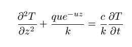
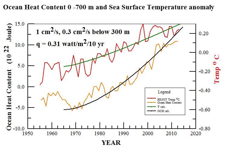
Figure 1. Ocean heat content 0 – 700 meter and surface temperature trends according to NOAA. Blue and green lines show trends calculated for the parameters shown.
These calculations establish some parameters that do a good job of representing the thermal behavior of the upper oceans, however, if one looks closely at the data trends in the graph, it is apparent that both surface temperature and ocean heat content have considerably slowed their rates of increase in the last decade. This makes it unlikely that greenhouse gases are the cause of the rate of heating needed to explain the previous trends because their effects should have become enhanced rather than diminished. It might also be noted that a similar warming trend occurred in the first half of the previous century before anthropogenic greenhouse gases could have contributed significantly. Thus it is more likely that both warming periods had natural origins.
Obtaining simultaneous fits to the ocean heat content and sea surface temperature trends with only two free parameters, thermal diffusivity and surface heating rate, is quite confining. Acceptable, but noticeably worse, fits than shown above, were obtained with thermal diffusivities ranging from 0.8 to 1.2 cm2/s and heat inputs ranging from 0.29 to 0.33 watt/m2. Based on previous calculations for sea level data, I was initially inclined to think that larger thermal diffusivities would be necessary, but larger values let more heat penetrate to greater depths than the amounts of heat reported by Levitus et al. In addition, I was chagrined to learn that most of the variation of sea level that accompanies solar cycles is caused by evaporation rather than thermal expansion.
Solar Cycles:
The process of choosing thermal diffusivity and surface heating rates to accord with observations provides a sound basis for calculating what to expect for the temperature variations during solar cycles. In this case we can use the thermal diffusivity of 1 cm2/s that is required of the ocean heat content results as an input parameter and choose the heat input that is required to produce temperature variations of 0.04 – 0.05 oC amplitude. Producing sea surface temperature variations with an amplitude of 0.04 oC requires a surface heat input of 0.33 watt/m2, as shown below:
http://i1244.photobucket.com/albums/gg580/stanrobertson/solarcycle10_zpsa3b8b0ee.jpg
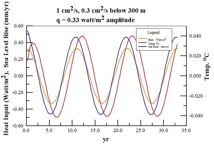

Figure 2. Radiant flux, ocean temperature oscillations, and sea level variations for three solar cycles of eleven years each. The entering flux shown here is the value of q = 0.33 watt/m2 needed to drive the variations of surface temperature of 0.04 oC with ocean thermal diffusivity of 1.0 cm2/s to depth of 300 m. The amplitude of thermosteric rate of change of sea level was 0.47 mm/yr. Temperature lags the driving energy flux by 15 months. The thermal expansion coefficient of sea water used here was 2.4×10⁻⁴/ oC.
I believe that this settles the issue of what is required to produce sea surface temperature oscillations with an amplitude of 0.04 oC. The solar TSI variations that reach the earth’s surface are smaller than the 0.33 watt/m2 needed to account for sea surface temperature variations by a factor of 3.6 for this smallest estimate of sea surface temperature variability.
Although the estimated 0.33 watt/m2 that is required to explain the surface temperature variations is large compared to the amplitude of TSI variations that reach the surface, it is still only about two parts per thousand of the 160 watt/m2 of solar UV/VIS/NIR that reaches the earth surface. There are many possible ways in which the sun might modulate the surface energy flux to this extent. These include modulation of cloud cover and small spectral shifts in the energetic UV that might modulate ozone absorption or produce shifts of the effective sea surface albedo. It would seem to be a fairly direct radiative effect, rather than feedback, since it must vary in phase with the solar cycle.
In summary, my calculations based on energy conservation considerations imply that the sun modulates the ocean temperatures to a much greater extent than can be provided solely by its TSI variations. The great question that desperately needs an answer is how does it do it? It should be easily understood that solar effects would not necessarily be confined to cycles. More likely, the sun has been the driver of the large changes of temperatures of the Roman and Medieval warm period, the Little Ice Age, and the recent recovery from it without requiring large changes of its own irradiance. When we understand how the sun does this, we will have begun to understand the earthly climate.
###
Biographical note:
Stan Robertson, Ph.D, P.E, retired in 2004 after teaching physics at Southwestern Oklahoma State University for 14 years. In addition to teaching at three other universities over the years, he has maintained a consulting engineering practice for 30 years.
References:
Bryan, F., 1987: Parameter Sensitivity of Primitive Equation Ocean General Circulation Models. Journal of Physical Oceanography, 17, 970-985. (PDF available here http://journals.ametsoc.org/doi/abs/10.1175/1520-0485%281987%29017%3C0970%3APSOPEO%3E2.0.CO%3B2
Levitus, S. et al., 2012 World ocean heat content and thermosteric sea level change (0–2000 m), 1955–2010, Geophysical Research Letters, 39, L10603, doi:10.1029/2012GL051106, 2012 http://onlinelibrary.wiley.com/doi/10.1029/2012GL051106/abstract
Shaviv, Nir 2008, Using the oceans as a calorimeter to quantify the solar radiative forcing, Journal of Geophysical Research, 113, A11101 http://www.sciencebits.com/files/articles/CalorimeterFinal.pdf
Trenberth, K., Fasullo, J., Kiehl, J. 2009: Earth’s Global Energy Budget. Bull. Amer. Meteor. Soc., 90, 311–323. doi: http://dx.doi.org/10.1175/2008BAMS2634.1 www.cgd.ucar.edu/staff/trenbert/trenberth.papers/TFK_bams09.pdf , Fig. 1
Zhou, J. and Tung, K. ,2010 Solar Cycles in 150 Years of Global Sea Surface Temperature Data, Journal of Climate 23, 3234-3248 http://journals.ametsoc.org/doi/abs/10.1175/2010JCLI3232.1
J Martin says:
October 12, 2013 at 1:13 pm
At least two VEI 6 (Pinatubo order of magnitude) eruptions occurred during the Maunder Minimum (c. AD 1645 to 1715):
http://en.wikipedia.org/wiki/List_of_large_volcanic_eruptions
6 Long Island (Papua New Guinea) Bismarck Volcanic Arc 1660
6 Kolumbo, Santorini South Aegean Volcanic Arc Sep 27, 1650
milodonharlani says:
October 12, 2013 at 9:40 am
Jim G says:
October 12, 2013 at 7:31 am
“Undersea volcanism varies over time, of course. Air temperature in the Cretaceous, for instance, was warm, but not enough to heat the oceans to the degree observed in proxy data. Sea level was so high then not just because of lack of ice, but due to thermal expansion of the oceans, thanks to submarine volcanism-driven active seafloor spreading as the continents raced away from each other. They’re still doing that, of course, but not to the same extent as especially in the mid-Cretaceous.”
I cannot help but think that this, along with a multitude of other unknown quantities, might have a substantial and varying effect upon our climate over the shorter term, non-geologic time frames, just as land based volcanism does.
@milodonharlani
Also, another thought, since under sea activity injects heat directly into the water it would be much longer lasting in its effect than mere reflection of TSI components.
Jim G says:
October 12, 2013 at 5:15 pm
Submarine volcanism also has a long-term climatic effect, as I indicated for the Cretaceous. The split up of Gondwana let the sea in among the Americas, Europe & Africa, with active seafloor spreading between these formerly conjoined continents, thus heating these new seaways.
Jim G says:
October 12, 2013 at 5:22 pm
Indeed, especially when the heat injection process lasts for millions of years.
wayne says:
October 12, 2013 at 5:04 pm
have a very precise ability to measure momentary differences in the TSI the absolute accuracy, a different parameter
As I have pointed out already, the SORCE data has an absolute accuracy of 0.5 W/m2. For variations over time, what matters is the relative precision which is about a thousand times better. Earlier instruments had systematic errors [the precision aperture was in the wrong place allowing scattered light to enter the cavity thus giving too high values]. All this is now known and can be corrected for.
each here should at least have the opportunity to see such plots that raise a question outside of the leveling adjustments if there could be some misapplied assumptions involved
If you don’t care to read the explanation of the detection and correction of the systematic errors in older data, what does looking at the plots do for you? Here is the beef: http://www.leif.org/EOS/2010GL045777.pdf This is now a non-issue and no further misconceived questions should arise.
milodonharlani says:
I would assume that since the plates keep moving that it is a continuous process only varying in degree.
Jim G says:
October 12, 2013 at 5:30 pm
There is less volcanism when the plates are all run together, as during Pangaea. When that last supercontinent started splitting up, the oceans necessarily warmed up. Also, seafloor spreading doesn’t always occur at the same rate while it is going on, & as the Atlantic has gotten larger, the same amount of volcanism heats it relatively less per unit of volume.
For instance, the epicontinental seaways that spread & retreated across North America in the Jurassic & Cretaceous transgressed & regressed largely due to thermal expansion & contraction from varying degrees of volcanism. Extinction events both on land & in the seas are also often associated with, if not conclusively caused by, extensive rift volcanism. A notable example is the Triassic-Jurassic, one of the so-called Big Five.
Today plate rates of motion vary considerably, & have done so more in the past:
http://hypertextbook.com/facts/ZhenHuang.shtml
The Indian Plate has run into the Eurasian, lifting up the Himalayas, but before that it was a speed demon crossing the Indian Ocean from Antarctica, although at varying rates:
http://gji.oxfordjournals.org/content/early/2013/05/27/gji.ggt162.abstract
It passed over the Reunion Island Hot Spot around the end of the Mesozoic & start of the Cenozoic Eras, ie at the K-T mass extinction event. This caused the Deccan Traps flood basalts, implicated in that extinction, along with the bolide impact in the Yucatan.
lsvalgaard: Quote:The solar TSI variations that reach the earth’s surface are smaller than the 0.33 watt/m2 needed to account for sea surface temperature variations by a factor of 3.6 for this smallest estimate of sea surface temperature variability.
Reply:So, in normal science, that falsifies the assumption that solar variations are the cause.
So what causes the Earth mean temp, sea surface rise and ohc to fluctuate in synchrony with the solar cycle? Did you dispute that the synchrony has occurred?
What his calculations show is that in the standard model (time-and-area-averaged insolation, time-and-area-averaged response, etc), the Earth effect can not be obtained from the direct effect of the small TSI change. If the non-linearity of the dynamic response (Equator vs poles, day vs night, radiation vs vaporization, etc) is inaccurately modeled, then the fault is in the Earth model, not the claim that the fluctuations in TSI are responsible. If the effect of TSI is real, then the mechanism must be an indirect effect such as cloud-cover change. Only if the entire model is complete and accurate does this result show that solar variations are not the cause.
lsvalgaard: Quote: For a start, here’s 50 papers describing potential solar amplification mechanisms
Reply:None of those explain how 3.6 times more heat reach the surface than the variation of what the Sun puts out…Otherwise the climate system would be a nifty energy producer: you put 10 units in and you get 36 out. I want one of those 🙂
If some component of insolation causes variation in the cloud cover, then that component is acting more like a component of a triode, pentode, or transistor than like an amplifier.
Right now, evidence for and against such indirect mechanisms is not very complete. To claim that they can’t exist on the scale required to account for the Sun’s effects is premature.
lsvalgaard: The albedo is basically determined by clouds. It takes a lot of energy to make clouds. The solar wind does not have a lot of energy.
It is helpful to cloud formation if there are condensation nuclei, and the variation in the solar wind probably has some effect on those.
Leif Svalgaard, I think that you have shown conclusively that a direct effect of tiny variations of TSI on the Earth surface, expressed with respect to the standard simplified model of the mean Earth, is not demonstrated by the main post. As was admitted and shown in the main post. Your arguments that there can be no indirect effects by components of the solar radiation, broadly considered, are exclusively restatements of the fact that there is no evidence for a direct effect within the constraints of the standard model.
Whether mechanisms to account for a non-negligible, indirect effect is a research area with important unanswered questions.
Yes Leif, all should also also read http://www.leif.org/EOS/2010GL045777.pdf . Sorry I didn’t include that KL2010 paper and everyone should read it very carefully, I have before.
It is about TSI and the instruments that measure it, and you would think such a paper should be devoid of repeated mentions and ties to the like of IPCC, analyses of global surface temperatures, CRU, human anthropogenic warming and such, but it isn’t. I for one will await time to pass to see if this was all performed correct and proper.
One thing that raised my eyebrows in that paper was the mention that the previous radiometers were letting 2-3x (200-300%) the solar irradiance than what they were actually measuring yet the warmer readings were a mere 0.13% warmer. You would think it would be much more that reported. I’ll just keep that paper on hold for future confirmations or corrections.
It is interesting, in Leif’s link, figure 3a how PMOD, ACRIM and TIM show an almost identical fluctuation pattern since 2003, with TIM having the lower offset. They say that their aim is to increase the stability with time by a factor of ten which sounds good for future TSI readings. Wish we could do likewise with land/sea temperatures.
The article concludes
Quite a difference.
Ulric Lyons says:
October 12, 2013 at 6:38 am
Tom in Florida says:
“..vast ocean circulation and large annual temperature ranges that all happen at different times and places around the Earth and that are caused by things other than the Sun.”
Unless of course solar plasma variability effects pressure systems and the jet stream latitude and equatorial winds, then it would be forcing the AMO and ENSO.
——————————————————————————————————————
You forgot to post the link to the reference paper from which you are getting your information.
Matthew R Marler says:
October 12, 2013 at 6:07 pm
So what causes the Earth mean temp, sea surface rise and ohc to fluctuate in synchrony with the solar cycle? Did you dispute that the synchrony has occurred?
I have always said that the small variation of TSI is just enough to explain the small solar cycle variation of climate, but since that effect is observed to be small the Sun is not the driver of the much larger [and therefore important] variations that have taken place.
Right now, evidence for and against such indirect mechanisms is not very complete. To claim that they can’t exist on the scale required to account for the Sun’s effects is premature.
I say that they exist and have just the right size to explain the observed variation. The authors of the article [and many commenters and you, it seems] dispute that. Go figure.
is not demonstrated by the main post.
The main post denies that the variation of TSI explains the observed variation. I say that the observed variation on the time scale of a solar cycle is neatly explained by the variation of TSI. You seem to deny that.
wayne says:
October 12, 2013 at 6:38 pm
I for one will await time to pass to see if this was all performed correct and proper.
If you cannot see everything is above board and done properly now, then you can wait forever.
One thing that raised my eyebrows in that paper was the mention that the previous radiometers were letting 2-3x (200-300%) the solar irradiance than what they were actually measuring yet the warmer readings were a mere 0.13% warmer.
I don’t know where you get the 200-300% from. This is just wrong.
Keith Minto says:
October 12, 2013 at 7:03 pm
This new value, measured by SORCE/TIM….Quite a difference.
But the variation with time does not have that large difference and that is the most important. It is like your measuring the height of a wave on the surface of the sea to be 10 feet, but when you measure it from the bottom of the sea [5000 feet down] it will be 5010 feet. Then re-measurement of the sea bottom profile now shows that the bootom is actually 5015 feet down, so now the wave height is 5025 feet, but the wave you see at the surface is still only 10 feet, regardless of how deep the sea is…
UKSP Nugget: What is our current understanding of solar irradiance variations?
The thermal efficiency parameters calculated from this experimental data could result in an uncertainty of ±2.5 W/m² on TSI values:
http://www.issibern.ch/teams/solarirradiance/Meeting2_Presentations/DIARAD_Sabri.pdf
AJB says:
October 12, 2013 at 10:02 pm
The thermal efficiency parameters calculated from this experimental data could result in an uncertainty of ±2.5 W/m² on TSI values
On the DIARAD TSI values, luckily not on the SORCE/TIM series.
lsvalgaard says: October 12, 2013 at 10:07 pm
Sure, but will this not have an effect on reassessment of composites like PMOD?
From that link, AJB
and
Together with a discussion of the wavelength limitations of SORCE, brings us closer to answering my original question.
The TSI variance seems to getting larger, not smaller.
lsvalgaard says:
October 12, 2013 at 8:48 pm
Ok, you will find that on page 4 of 7 near the bottom:
Excerpt:
Well, yes, of course you would expect some warming effect on the instrument since dealing with direct solar radiation in the void of space. I’m just a bit surprised they found it was that small 0.0013 fraction of spurious warming in the readings. Maybe there was refrigeration to remove heat but I don’t see such fine details such as specific design descriptions.
Leif, I normally accept papers at their face value knowing all of the work that goes into them. But as we have seen over and over again in climate science especially propping IPCC’s entire reason to exist and you had better not do so at face value. I’m just sorry this paper had to be a mix of the two and I could trust it more.
Keith Minto says, October 12, 2013 at 10:51 pm
bit chilly says: October 12, 2013 at 4:10 pm
allan macrae, a fantastic series of posts . an education in themselves. thank you.
____________
Allan says: Thank YOU Chilly for your kind words.
The one certainty in this difficult and often-fractious debate on Earth’s climate and its causes and effects, is that we are all in this together.
I recall as a young man, in a moment of temporary youthful despair, walking into student housing and seeing this on the wall:
‘No Man is an Island’
No man is an island alone unto itself;
Every man is a piece of the continent, a part of the main;
If a clod be washed away by the sea,
Europe is diminished,
Even as a promontory were,
Even as a Manor of thy friends or of thine own were;
Any man’s death diminishes me,
Because I am involved with mankind.
And therefore send not to know for whom the bell tolls;
It tolls for thee.
***********
There was no attribution to an author.
I later determined that this was an edited modern version of Meditation XVII, Devotions upon Emergent Occasions, by John Donne.
I recall that these eloquent words put my (probably trivial) problem of the moment into better perspective.
But what really struck me at the time was the date of publication – 1624* – and the modernity of the ideas in a time of rigid social hierarchy and great violence at all levels of society.
Best regards, Allan
* James I was King, son of Mary Queen of Scots, beheaded by Elizabeth I, daughter of Henry VIII, who also tended to behead those who fell into disfavour. To his credit, Henry only beheaded two of his six wives. Apart from his wives and many others, Henry beheaded Sir Thomas Moore in 1535. More had in 1516 published the book “Utopia” which also espoused concepts of society that were remarkably modern for their time.
Keith Minto says:
October 12, 2013 at 10:51 pm
The SORCE mission is reaching an end so, for now, the potential range of solar cycle spectral variability is likely to remain quite large and therefore uncertainty will remain in the impact it has on the Earth’s climate system.
You are confusing TSI with SSI [the spectral variability, i.e. the variation with wavelength of the irradiance]. SSI is very difficult to measure. The errors are of the order of 10% or more, while the error on TSI is thousands of times smaller.
Together with a discussion of the wavelength limitations of SORCE, brings us closer to answering my original question.
There are no wavelength limitations in SORCE/TSI.
The TSI variance seems to getting larger, not smaller.
Again confusion of SSI and TSI.
wayne says:
October 12, 2013 at 10:56 pm
Additionally, this design allows into the instrument interior two to three times the amount of light intended to be measured; if not completely absorbed or scattered back out, this additional light produces erroneously high signals.
The interior has a system of baffles designed to eliminate this extra light, but a small fraction gets by anyway. SORCE/TIM does not have that problem.
Leif, I normally accept papers at their face value knowing all of the work that goes into them. But as we have seen over and over again in climate science especially propping IPCC’s entire reason to exist and you had better not do so at face value. I’m just sorry this paper had to be a mix of the two and I could trust it more.
The remedy is simple: read the paper and the supporting documentation. Your default assumption [that all papers cannot be trusted] is wrong. Now, it is a too easy excuse to blame the data producers for conspiracy and monkey business, but in case of SORCE/TSI that excuse is not valid. And the paper does not ‘mix the two’. On the contrary, it is critical of the models used by IPCC: “This response is larger by a factor of 2 or more than in the current models assessed by IPCC [Tung et al., 2008], possibly because of the models’ excessive heat uptake by the ocean”.