 (Perturbation Calculations of Ocean Surface Temperatures.)
Guest essay by Stan Robertson, Ph.D., P.E.
1. Introduction
It is generally conceded that the earth has warmed a bit over the last century, but it is not clear what has caused it, nor whether it will continue and become a problem for humanity. There is a possibility that some of the warming has been caused by anthropogenic greenhouse gases, but it is also likely that the sun has been partially responsible. The arguments that are advanced to say that humans caused it and that it will become a serious problem rely on models that have not been validated and positive feedback effects that have not been shown to exist, at least at the hypothesized levels of effectiveness. The apparent weakness in the argument that the sun has been a major contributor is that satellite measurements of Total Solar Irradiance (TSI) have not shown changes large enough to have directly produced the warming of the earth over the last half century. But what about indirect effects? Is it possible that the sun exerts control in some indirect way? In these notes I recapitulate the evidence that this is the case by showing that the variations of TSI cannot provide the energy that is necessary to account for the warming of the oceans during solar cycles.
TSI, as measured above the earth’s atmosphere varies by about 1.2 watt/m2 over a nominal eleven year solar cycle (h/t Leif Svaalgard) primarily at wavelengths shorter than 2 micron. The dominant harmonic variation of TSI would thus have an amplitude half this large, or about 0.6 watt/m2. About 70% of this enters the earth atmosphere. Averaged over latitudes and day/night cycles, about one fourth of this 70%, or ~0.11 watt/m2, on average, enters the upper atmosphere. Since only about 160 watt/m2 of 1365 watt/m2 of incoming solar radiation at wavelengths less than 2 micron reaches the earth surface, the amplitude of short wavelength TSI reaching the earth surface would be only (160/1365)x0.6 = 0.07 watt/m2. However, about half of the difference between 0.11 and 0.07 watt/m2 eventually reaches the earth surface as scattered thermal infrared radiation at wavelengths greater than 2 micron. Thus the average amplitude of TSI reaching the earth surface in all wavelengths would be about 0.09 watt/m2. So the question is, just how much sea surface temperature variation can this produce?
Several researchers, including Nir Shaviv (2008), Roy Spencer (see http://www.drroyspencer.com/2010/06/low-climate-sensitivity-estimated-from-the-11-year-cycle-in-total-solar-irradiance/) and Zhou & Tung (2010) have found that ocean surface temperatures oscillate with an amplitude of about 0.04 – 0.05 oC during a solar cycle. (In fact, all of the ideas that I am presenting here were covered in Shaviv’s work, but it has not gotten the attention that it deserves.) Using 150 years of sea surface temperature data, Zhou & Tung found 0.085 oC warming for each watt/m2 of increase of TSI over a solar cycle. Although not strictly sinusoidal, the temperature variations can be approximately described in terms of a dominant sinusoidal component of variation with an 11 year period. Thus the question to be answered at this point is, can 0.09 watt/m2 amplitude of variation of TSI entering the oceans produce temperature oscillations with an amplitude of 0.04 – 0.05 oC?
The answer to this question depends on the average thermal diffusivity of the upper oceans. That is an unknown, but not unknowable, quantity. Thermal diffusivity is the ratio of thermal conductivity to heat capacity. The upper 25 to 100 meters of oceans are well mixed by waves and shears. These are mixing zones with high thermal diffusivity and correspondingly small temperature gradients. Diffusivities are lower at greater depths. Bryan (1987) has found that thermal diffusivities ranging from 0.3 to 5 cm2/s are needed to account for the temperature profiles below the mixing zone. In my first trial calculations of the energy flux necessary to account for the temperature variations, I tried values of thermal diffusivity in the range 0.1 – 10 cm2/s and found that the TSI variations were generally inadequate to produce the sea temperature variations over a solar cycle. But there was wide variation of calculated energy flux. Larger values of thermal diffusivity required more heat because more was able to penetrate to the depths, but even for 0.1 cm2/s, the required input was double the TSI variations that reach the earth surface. Fortunately, there is a way to constrain both the value of the thermal diffusivity and the heat input. It consists of first matching the measured trends of surface temperatures and ocean heat content over time. Measurements of these were reported by Levitus et al. (2012) and are available from http://www.nodc.noaa.gov/OC5/3M_HEAT_CONTENT/ .
In the calculations described below, I have used the data from 1965 to 2012 for ocean depths to 700 meters. Sea surface temperatures and ocean heat content began to increase after 1965. Only about a third of the increase of heat content occurred at depths below 700 meter. Since little heat migrates below this depth over 11 year solar cycles, it is preferable to use the 0 – 700 m data for the purpose of calibrating the thermal diffusivity
2. Heat Transfer Perturbation Calculations
For the calculation of sea surface temperature and sea level changes, we can treat the variations of radiations entering and leaving atmosphere, lands and oceans as minor perturbations on an earth essentially in thermal equilibrium. Ocean mixing zones, thermoclines and other features of the temperature profiles remain largely as they were while small radiant disturbances produce minor variations of temperature starting from zero, and imposed at each depth. Thus the effects of these disturbances can be modeled as one-dimensional energy flows into a medium at uniform temperature. Such “perturbation calculations” are among the most powerful analysis techniques used by physicists and engineers and are widely used. The energy equation to be solved in this case is:
http://i1244.photobucket.com/albums/gg580/stanrobertson/equation_zpscea297ad.jpg

Where T is the temperature departure from equilibrium at depth , z, and time, t. q is a perturbing radiant flux entering the surface, u the absorption coefficient, c is absorber heat capacity and k its thermal conductivity. The rate of heat transfer by conduction processes is controlled by the thermal diffusivity, which is the ratio k/c.
As a one dimensional heat flow problem, it is straightforward undergraduate level physics or engineering to numerically solve the equation above for the expected changes of surface temperature as surface radiant flux varies. In my calculations, temperature changes were calculated for 1.0 meter increments of depth in the oceans. Two cases were considered. In one
case the surface radiation perturbation was assumed to increase linearly with time. This corresponds to the ocean conditions for the period 1965-2012. In the second case, it was assumed to vary as a cosine function of time with the 11 year period of the solar cycle. The cosine function provides both some positive and some negative variation in the first half cycle, which helps to minimize the transients of the first few years.
I treated q and thermal diffusivity, (k/c), as input parameters that were chosen to provide agreement with the observed sea surface temperature variations and ocean heat content measurements (https://www.ncdc.noaa.gov/ersst/ ). The absorption coefficient, u, was entered in piecewise fashion. Only the deep UV radiations penetrate to depths below 10 meter, but conduction takes energy to much greater depths. For the values of u chosen, only 44.5% of the surface energy flux goes deeper than 1 meter, 22.5% below 10 meter and 0.53% to 100 meter (h/t Leif Svalgaard). Thermal diffusivity of oceans was assumed to be 0.3 cm2/s below 300 m. This accords with Bryan’s estimates below the mixing zone, but little change of results occurred for values as low as 0.1 cm2/s. The required heat inputs are relativity insensitive to the thermal diffusivity below 300 meter. For the shallower depths, thermal diffusivity was varied until trends in accord with observed temperatures and heat content were produced.
It is necessary to maintain an energy balance at the sea surface in approximate equilibrium with the incoming solar radiation. As estimated by Trenberth, Fasullo and Kiehl (2009), about 160 watt/m2 enters the surface, on average. At a mean temperature of 288 oK, the sea surface will emit about 390 watt/m2 of surface thermal infrared radiation at wavelengths longer than about 2 micron, however, about 84% of that is returned as back scattered radiation. The rest of the energy balance is provided by evaporation and thermal convection, which remove about 59% of the heat from the surface. From the standpoint of merely wanting to know how much heat is required to change the ocean surface temperature, it is possible to maintain a proper energy balance without delving into the messy details of evaporation, convection and infrared absorption in the first few millimeters of water. The temperature variations at one meter depth will not be measurably different from those at the surface for the thermal diffusivities of interest here. If we merely want to know what net energy flux entering the surface is required to make the water temperature at one meter depth oscillate with an amplitude of 0.04 – 0.05 oC , then all we need to do is account for the outgoing surface infrared emission and let 41% (160 watt/m2 / 390 watt/m2 = 0.41) escape. At the present 288 oK, the earth radiates an additional 5.42 watt/m2 for each 1 oC increase of surface temperature. In the case of surface temperature being perturbed by 0.04 oC, an outgoing additional 0.22 watt/m2 would be generated and 0.09 watt/m2 was allowed to escape. This nicely balances the amplitude of TSI variations that reach the earth’s surface.
3. Linear heating:
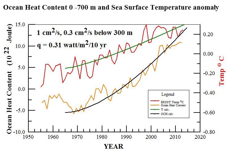
In these calculations, the aim was to find the heat input and thermal diffusivities necessary to account for the observed surface temperature increase (http://www.nodc.noaa.gov/OC5/3M_HEAT_CONTENT/ )Extended Reconstructed Sea Surface Temperature) and the increased ocean heat content (OHC 700) that have been reported by NOAA. Since surface temperatures had not been increasing in the early 1960s, but began to increase in the last half of that decade, I chose to start calculations with linearly increasing heating in 1965. I found that the ocean heat content to a depth of 700 meters was quite sensitive to the thermal diffusivity used. The best results that I have been able to obtain were for a thermal diffusivity of 1 cm2/s to 300 meter depth and surface heat input increasing at a rate of 0.31 watt/m2 per decade. These are shown on the graph below with calculated trends shown by the green and black lines. On a time scale of 50 years, most of the heat accumulates at relatively shallow depths. To better reflect a realistic thermal diffusivity for greater depths, I used a lower value of 0.3 cm2/s below 300 meter. That has little practical effect on a 50 year times scale, but would be necessary if one wanted to extend the calculations for several centuries while surface heating perturbations had time to penetrate to much greater depths.
http://i1244.photobucket.com/albums/gg580/stanrobertson/OHC700_zpsb9e34e91.jpg

Figure 1. Ocean heat content 0 – 700 meter and surface temperature trends according to NOAA. Blue and green lines show trends calculated for the parameters shown.
These calculations establish some parameters that do a good job of representing the thermal behavior of the upper oceans, however, if one looks closely at the data trends in the graph, it is apparent that both surface temperature and ocean heat content have considerably slowed their rates of increase in the last decade. This makes it unlikely that greenhouse gases are the cause of the rate of heating needed to explain the previous trends because their effects should have become enhanced rather than diminished. It might also be noted that a similar warming trend occurred in the first half of the previous century before anthropogenic greenhouse gases could have contributed significantly. Thus it is more likely that both warming periods had natural origins.
Obtaining simultaneous fits to the ocean heat content and sea surface temperature trends with only two free parameters, thermal diffusivity and surface heating rate, is quite confining. Acceptable, but noticeably worse, fits than shown above, were obtained with thermal diffusivities ranging from 0.8 to 1.2 cm2/s and heat inputs ranging from 0.29 to 0.33 watt/m2. Based on previous calculations for sea level data, I was initially inclined to think that larger thermal diffusivities would be necessary, but larger values let more heat penetrate to greater depths than the amounts of heat reported by Levitus et al. In addition, I was chagrined to learn that most of the variation of sea level that accompanies solar cycles is caused by evaporation rather than thermal expansion.
Solar Cycles:
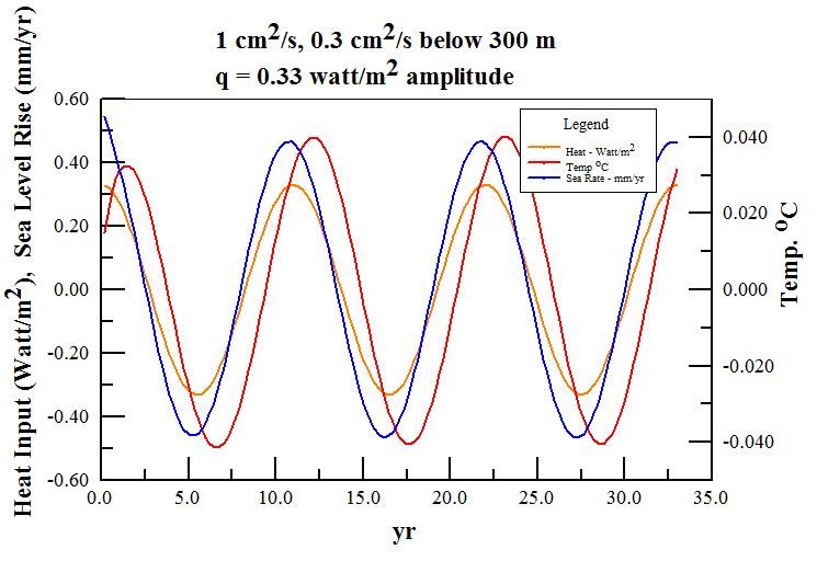
The process of choosing thermal diffusivity and surface heating rates to accord with observations provides a sound basis for calculating what to expect for the temperature variations during solar cycles. In this case we can use the thermal diffusivity of 1 cm2/s that is required of the ocean heat content results as an input parameter and choose the heat input that is required to produce temperature variations of 0.04 – 0.05 oC amplitude. Producing sea surface temperature variations with an amplitude of 0.04 oC requires a surface heat input of 0.33 watt/m2, as shown below:
http://i1244.photobucket.com/albums/gg580/stanrobertson/solarcycle10_zpsa3b8b0ee.jpg

Figure 2. Radiant flux, ocean temperature oscillations, and sea level variations for three solar cycles of eleven years each. The entering flux shown here is the value of q = 0.33 watt/m2 needed to drive the variations of surface temperature of 0.04 oC with ocean thermal diffusivity of 1.0 cm2/s to depth of 300 m. The amplitude of thermosteric rate of change of sea level was 0.47 mm/yr. Temperature lags the driving energy flux by 15 months. The thermal expansion coefficient of sea water used here was 2.4×10⁻⁴/ oC.
I believe that this settles the issue of what is required to produce sea surface temperature oscillations with an amplitude of 0.04 oC. The solar TSI variations that reach the earth’s surface are smaller than the 0.33 watt/m2 needed to account for sea surface temperature variations by a factor of 3.6 for this smallest estimate of sea surface temperature variability.
Although the estimated 0.33 watt/m2 that is required to explain the surface temperature variations is large compared to the amplitude of TSI variations that reach the surface, it is still only about two parts per thousand of the 160 watt/m2 of solar UV/VIS/NIR that reaches the earth surface. There are many possible ways in which the sun might modulate the surface energy flux to this extent. These include modulation of cloud cover and small spectral shifts in the energetic UV that might modulate ozone absorption or produce shifts of the effective sea surface albedo. It would seem to be a fairly direct radiative effect, rather than feedback, since it must vary in phase with the solar cycle.
In summary, my calculations based on energy conservation considerations imply that the sun modulates the ocean temperatures to a much greater extent than can be provided solely by its TSI variations. The great question that desperately needs an answer is how does it do it? It should be easily understood that solar effects would not necessarily be confined to cycles. More likely, the sun has been the driver of the large changes of temperatures of the Roman and Medieval warm period, the Little Ice Age, and the recent recovery from it without requiring large changes of its own irradiance. When we understand how the sun does this, we will have begun to understand the earthly climate.
###
Biographical note:
Stan Robertson, Ph.D, P.E, retired in 2004 after teaching physics at Southwestern Oklahoma State University for 14 years. In addition to teaching at three other universities over the years, he has maintained a consulting engineering practice for 30 years.
References:
Bryan, F., 1987: Parameter Sensitivity of Primitive Equation Ocean General Circulation Models. Journal of Physical Oceanography, 17, 970-985. (PDF available here http://journals.ametsoc.org/doi/abs/10.1175/1520-0485%281987%29017%3C0970%3APSOPEO%3E2.0.CO%3B2
Levitus, S. et al., 2012 World ocean heat content and thermosteric sea level change (0–2000 m), 1955–2010, Geophysical Research Letters, 39, L10603, doi:10.1029/2012GL051106, 2012 http://onlinelibrary.wiley.com/doi/10.1029/2012GL051106/abstract
Shaviv, Nir 2008, Using the oceans as a calorimeter to quantify the solar radiative forcing, Journal of Geophysical Research, 113, A11101 http://www.sciencebits.com/files/articles/CalorimeterFinal.pdf
Trenberth, K., Fasullo, J., Kiehl, J. 2009: Earth’s Global Energy Budget. Bull. Amer. Meteor. Soc., 90, 311–323. doi: http://dx.doi.org/10.1175/2008BAMS2634.1 www.cgd.ucar.edu/staff/trenbert/trenberth.papers/TFK_bams09.pdf , Fig. 1
Zhou, J. and Tung, K. ,2010 Solar Cycles in 150 Years of Global Sea Surface Temperature Data, Journal of Climate 23, 3234-3248 http://journals.ametsoc.org/doi/abs/10.1175/2010JCLI3232.1
Salvatore Del Prete says:
October 12, 2013 at 9:45 am
I detected good idea from what you write – that the last decade and bit of nonwarming can serve as example for limited equilibrium state and if further “slump” in solar activity occurs (which is quite likely as the cycle will reach its end), then cooling will occur. Do I interpret it well?
Yes, that is what I suggest. There must be or I should say there are threshold values of change in solar activity that will impact the climate. The question is what are all those values and what kind of a duration do they require?
To make my point if the sun suddenly went dead we would all agree the earth would be frozen, therefore showing the sun does effect the climate at some point of change.
Now the question is how little of a change is needed in all the solar parameters to change the climate of the earth through primary solar changes and the secondary effects associated with those primary solar changes?
I suggest it is the solar average parameters I have listed which I think are similar to previous prolonged solar minimum periods which have impacted the climate in the past, if one looks at past history.
[snip – don’t accuse Dr. Svalgaard of impropriety without basis – take a 48 hour time out from WUWT – Anthony]
wayne says:
October 11, 2013 at 10:06 pm
You sure that was not a trick question and I just fell for it?
========
No, it wasn’t intended as a trick and thank you to Leif for taking the time to answer, as it has given me insight into the problem.
Consider this paradigm:
P = Perfect knowledge of the Sun (god view, present, past and future)
This might be considered the ultimate goal of science. To fully know the past history of the sun, the internal processes, how it affects the earth, and to be able to predict this going forward without error.
Our current paradigm (C) is less complete. We know something about the subjects above, and some of what we know is correct, but if the history of science tells us anything, it is that some of what we believe to be correct is incorrect.
It is this incorrect knowledge that I left out of my original question, and I realize now that it is perhaps the most important part. The reason being is that incorrect knowledge acts in a fashion like negative or “anti-knowledge”. New ideas that conflict with the false beliefs are held back, because they contradicts what we believe to be true.
Lets incorporate correct (True) and incorrect (False) knowledge. We now have:
P = perfect paradigm
K = known in perfect paradigm (true knowledge)
U = unknown in perfect paradigm (true unknowns)
C = current paradigm
K(C) = known in current paradigm
U(C) = unknown in current paradigm
F(C) = known in current paradigm but false in perfect paradigm (false knowledge)
T(C) = known in current paradigm and true in perfect paradigm (true knowledge)
where K(C) = F(C) + T(C)
From this we can say
K = K(C) – F(C) (true knowledge = current knowledge – false knowledge)
U = U(C) + F(C) (true unknowns = current unknowns + false knowledge)
History shows us that F(C) > 0, therefore it can be said that:
U > U(C) = 0.5 (from Leif)
that the true unknowns are greater than what we believe.
Rhys Jaggar says:
October 12, 2013 at 10:27 am
Are there any wavelengths within the TSI which alter radically depending on the strength of the solar cycle?? … The 10.7cm radio flux is clearly one, but presumably there might be others also??
10.7, UV, and cosmic rays vary linearly with the solar cycle
Allan MacRae says:
October 12, 2013 at 10:23 am
This does not preclude the possibility that the observed increase in atmospheric CO2 is primarily caused by some factor (natural and/or humanmade) other than temperatures, but such increase in CO2 is insignificant to Earths’ temperatures. In summary, in climate science we do not even agree on what drives what…
I would think that the estimations of the anthropogenic emissions clearly exceed the rate of rise of its content in the atmosphere.
Where the surplus CO2 in atmosphere is coming from is in my opinion clear – it is anthropogenic – for example in 2008 from the global emissions estimations were that there was 40% more anthropogenic emissions than the atmospheric level rise would suggest, in 2010 46%. So the rest must sink, not be released from nature by unknown drivers. But the sinks are unable to adapt so quickly. The sinks evidently start to saturate and while in 1989-1992 the seasonal “sink” was 6.3ppm, in 2009-2012 already only 5.6ppm, while real sink in 2010 was 2.1ppm, the anthropogenic surplus was 4.5ppm. From the numbers is clear that nature is unable to keep up with the emissions development.
But it all of course doesn’t say anything about dominant cause of the recent warming. Also we should pose ourselves question how long into the future the emissions rate can last with the known fossil carbon reserves. I would think not more than another 25years. It will still not be by far enough for sink saturation and I even seriously doubt the infamous “doubling” from the preindustrial levels is ever achievable -at least not with the known fossil reserves. So to me the “problem” with the anthropogenic CO2 emissions looks like non-issue – even the rising level of atmospheric CO2 is clearly overwhelmingly if not only caused by it. The CO2 is unable to poison the nature – in fact the opposite is true and green flora thrives on it, so whenever the fossil reserves are depleted, the surplus CO2 atmospheric content will simply sink again, maybe even with accelerated rate given by previous fertilization, and that’s it. I think much more actual problem is how this technological civilization will survive the fossil carbon resources depletion.
Salvatore Del Prete says: October 12, 2013 at 9:45 am
tumetuestumefaisdubien1 says: October 12, 2013 at 10:38 am
I detected good idea from what you write – that the last decade and bit of non-warming can serve as example for limited equilibrium state and if further “slump” in solar activity occurs (which is quite likely as the cycle will reach its end), then cooling will occur. Do I interpret it well?
Salvatore Del Prete says: October 12, 2013 at 10:48 am
Yes, that is what I suggest…
Allan says:
One faction (to which I belong) says that global cooling will soon resume, or has already commenced.
I (we) predicted imminent global cooling in an article written in 2002.
So I agree with Salvatore above.
What will happen then?
Will global cooling be mild or severe?
I suggest cooling could be similar to the Dalton Minimum, which coincided with an average 1 degree C decline in global average temperature and caused significant human suffering.
But the Dalton also included the Tambora eruption in 1816, one of the largest volcanoes in the past 2000 years. The year 1816 was called The Year Without a Summer.
Just in case, bundle up!
Regards, Allan
From wiki:
Year Without a Summer
This article is about the year 1816..
The Year Without a Summer (also known as the Poverty Year, The Summer that Never Was, Year There Was No Summer, and Eighteen Hundred and Froze to Death[1]) was 1816, in which severe summer climate abnormalities caused average global temperatures to decrease by 0.4–0.7 °C (0.7–1.3 °F),[2] resulting in major food shortages across the Northern Hemisphere.[3][4] It is believed[by whom?] that the anomaly was caused by a combination of a historic low in solar activity with a volcanic winter event, the latter caused by a succession of major volcanic eruptions capped by the 1815 eruption of Mount Tambora, in the Dutch East Indies (Indonesia), the largest known eruption in over 1,300 years. The Little Ice Age, then in its concluding decades, may also have been a factor.[attribution needed]
The Year Without a Summer was an agricultural disaster. Historian John D. Post has called this “the last great subsistence crisis in the Western world”.[5] The unusual climatic aberrations of 1816 had the greatest effect on the northeastern United States, Atlantic Canada, and parts of western Europe. Typically, the late spring and summer of the northeastern U.S. and southeastern Canada are relatively stable: temperatures (average of both day and night) average between about 68 °F (20 °C) and 77 °F (25 °C) and rarely fall below 41 °F (5 °C). Summer snow is an extreme rarity.
In the spring and summer of 1816, a persistent “dry fog” was observed in the northeastern US. The fog reddened and dimmed the sunlight, such that sunspots were visible to the naked eye. Neither wind nor rainfall dispersed the “fog”. It has been characterized as a stratospheric sulfate aerosol veil.[6]
At higher elevations, where farming was touch and go in good years, the cooler climate did not quite support agriculture. In May 1816,[1] frost killed off most crops, on June 4 frosts were reported in Connecticut, and by the following day most of New England was gripped by the cold front.[7] On June 6, snow fell in Albany, New York, and Dennysville, Maine.[8]
Many commented on the phenomenon. Sarah Snell Bryant, of Cummington, Massachusetts, wrote in her diary, “Weather backward.” Samuel Griswold Goodrich said the summer of 1816 in Connecticut was the coldest of the century.[9]
At the New Lebanon, New York Church Family of Shakers, Nicholas Bennet wrote in May 1816 that “all was froze” and the hills were “barren like winter.” Temperatures went below freezing almost every day in May. The ground froze solid on June 9. On June 12, the Shakers had to replant crops destroyed by the cold. On July 7 it was so cold that everything had stopped growing. The Berkshire Hills had frost again on August 23.[10]A Massachusetts historian summed up the disaster: “Severe frosts occurred every month; June 7th and 8th snow fell, and it was so cold that crops were cut down, even freezing the roots …. In the early Autumn when corn was in the milk it was so thoroughly frozen that it never ripened and was scarcely worth harvesting. Breadstuffs were scarce and prices high and the poorer class of people were often in straits for want of food. It must be remembered that the granaries of the great west had not then been opened to us by railroad communication, and people were obliged to rely upon their own resources or upon others in their immediate locality.”[11]
Farther north, nearly 12 inches (30 cm) of snow was observed in Quebec City in early June, with consequent additional loss of crops—most summer-growing plants have cell walls which rupture even in a mild frost. The result was regional malnutrition, starvation, epidemic,[clarification needed] and increased mortality.
In July and August, lake and river ice were observed as far south as Pennsylvania. Rapid, dramatic temperature swings were common, with temperatures sometimes reverting from normal or above-normal summer temperatures as high as 95 °F (35 °C) to near-freezing within hours.
The weather was not in itself a hardship for hardy Yankees accustomed to long winters. The real problem lay in the weather’s effect on crops and thus on the supply of food and firewood.
Farmers south of New England did succeed in bringing some crops to maturity, but maize and other grain prices rose dramatically. The price of oats,[12] for example, rose from 12¢ a bushel ($3.40/m³) in 1815, equal to $1.53 today, to 92¢ a bushel ($26/m³) in 1816 ($12.65 today).
U.S. areas suffering crop failures also faced an inadequate transportation network, with few roads or navigable inland waterways and no railroads; it was expensive to import food.[13]
Cool temperatures and heavy rains resulted in failed harvests in Britain and Ireland as well. Families in Wales travelled long distances as refugees, begging for food. Famine was prevalent in north and southwest Ireland, following the failure of wheat, oats, and potato harvests. In Germany, the crisis was severe; food prices rose sharply. With the cause of the problems unknown, people demonstrated in front of grain markets and bakeries, and later riots, arson, and looting took place in many European cities. It was the worst famine of the 19th century.[8][14]
In China, the cold weather killed trees, rice crops, and even water buffalo, especially in the north. Floods destroyed many remaining crops. Mount Tambora’s eruption disrupted China’s monsoon season, resulting in overwhelming floods in the Yangtze Valley. In India the delayed summer monsoon caused late torrential rains that aggravated the spread of cholera from a region near the River Ganges in Bengal to as far as Moscow.[15]
In New York City, the temperature dropped to −26 °F (−32 °C) during the bitter winter of 1816-17. This resulted in a freezing of New York’s Upper Bay deep enough for horse-drawn sleighs to be driven across Buttermilk Channel from Brooklyn to Governors Island.[16]
The effects were widespread and lasted beyond the winter. In eastern Switzerland, the summers of 1816 and 1817 were so cool that an ice dam formed below a tongue of the Giétro Glacier high in the Val de Bagnes. Despite engineer Ignaz Venetz’s efforts to drain the growing lake, the ice dam collapsed catastrophically in June 1818.[17]
Allan MacRae says:
October 12, 2013 at 11:25 am
I suggest cooling could be similar to the Dalton Minimum, which coincided with an average 1 degree C decline in global average temperature and caused significant human suffering.
But the Dalton also included the Tambora eruption in 1815, one of the largest volcanoes in the past 2000 years. The year 1816 was called The Year Without a Summer.
Helped along with the eruption of Mayon in 1814 and another [unnamed] volcano erupting in 1809 http://onlinelibrary.wiley.com/doi/10.1029/2009GL040882/abstract
Obviously, I don’t predict a 1C decline [barring similar volcanic eruptions]
Allan MacRae says: October 12, 2013 at 10:23 am
This does not preclude the possibility that the observed increase in atmospheric CO2 is primarily caused by some factor (natural and/or humanmade) other than temperatures, but such increase in CO2 is insignificant to Earths’ temperatures. In summary, in climate science we do not even agree on what drives what…
tumetuestumefaisdubien1 says: October 12, 2013 at 11:13 am
I would think that the estimations of the anthropogenic emissions clearly exceed the rate of rise of its content in the atmosphere.
Where the surplus CO2 in atmosphere is coming from is in my opinion clear – it is anthropogenic – for example in 2008 from the global emissions estimations were that there was 40% more anthropogenic emissions than the atmospheric level rise would suggest, in 2010 46%. So the rest must sink, not be released from nature by unknown drivers. But the sinks are unable to adapt so quickly. The sinks evidently start to saturate and while in 1989-1992 the seasonal “sink” was 6.3ppm, in 2009-2012 already only 5.6ppm, while real sink in 2010 was 2.1ppm, the anthropogenic surplus was 4.5ppm. From the numbers is clear that nature is unable to keep up with the emissions development.
Allan says:
Hello tume, attributing the increase in atmospheric CO2 to the combustion of fossil fuels is called the “Mass Balance Argument” and it has been ably debated by Ferdinand Engelbeen (FOR) and Richard Courtney (NEUTRAL) here and elsewhere for years.
I am more or less NEUTRAL as well. Some days I am more neutral and some days I am less.
Got to go now.
Regards, Allan :-}
Some recent stuff:
http://wattsupwiththat.com/2013/10/08/the-taxonomy-of-climate-opinion/#comment-1440967
Gail Combs says:October 8, 2013 at 11:12 am
…Plants use all of the CO2 around their leaves within a few minutes leaving the air around them CO2 deficient, so air circulation is important. As CO2 is a critical component of growth, plants in environments with inadequate CO2 levels of below 200 ppm will generally cease to grow or produce… http://www.thehydroponicsshop.com.au/article_info.php?articles_id=27
Thank you Gail. Interesting.
http://wattsupwiththat.com/2013/08/11/murry-salby-responds-to-critics/#comment-1395118
(PLANT) FOOD FOR THOUGHT
CO2 is such a scarce and excellent plant food that it is gobbled up very close to the source during the growing season.
In urban environments like Salt Lake City where CO2 is emitted, it is gobbled up so quickly by plants that there is NO DISCERNIBLE HUMAN SIGNATURE IN THE DAILY CO2 RECORD.
For proof, see http://co2.utah.edu/index.php?site=2&id=0&img=31
Recognizing the CO2 is NOT that well-mixed in the atmosphere..
http://svs.gsfc.nasa.gov/vis/a000000/a003500/a003562/carbonDioxideSequence2002_2008_at15fps.mp4
… this may be where the “Mass Balance Argument” (fossil fuel combustion is the certain cause of atmospheric CO2 increases (NOT)) falls apart.
Let’s suppose that humanmade CO2 from fossil fuel combustion is quickly gobbled up by plants close to its (usually urban) source. The rest of the world and its carbon cycle just carries on, unaware in every way that humankind is burning fossil fuels. It also may be that humanity IS causing the observed increase in atmospheric CO2, but that increase may be due to other causes such as deforestation, agriculture, etc. Fossil fuel is just a convenient bogeyman – everyone hates the oil companies when they gas up their car – it’s just that the alternatives are worse.
Regards, Allan
The problem with Isvalgaards many answers is that he is arguing as apposed to considering or even debating. Valid arguments have been made and he ignores the majority picks a nit considers it done. TSI as measured is probably not as accurate as it could be. The data set has some obvious problems not the least of which is measuring something from within the atmosphere which is roughly considered to have particles out to 190,000km. The Sattelites are not in a direct line between earth and sun so there will be some scatter and waveform changes based on collisions. A small error could be significant.
Many others have made valid points.
What makes the article interesting is that there is an obvious correlation between the sun and SST’s. He makes a valid point that understanding where the failure between our measurements and reality lie is a key to understanding climate. Which we need to understand to avoid a lot of wrong ideas that we can hardly afford. The two biggest players in climate and long term trends is the SUN and Oceans. One provides the largest bit of energy and the other is a huge heat sink, this heat sink transports, stores and provides balance to the climate system.
So having a sharp shooter commenting to the negative on everything is really not helpful. If there are valid issues surely bring them up but don’t say things like 20 kilometers up and your out of the atmosphere, that is not good science.
David Riser says:
October 12, 2013 at 11:42 am
TSI as measured is probably not as accurate as it could be. The data set has some obvious problems not the least of which is measuring something from within the atmosphere which is roughly considered to have particles out to 190,000km. The Sattelites are not in a direct line between earth and sun so there will be some scatter and waveform changes based on collisions. A small error could be significant.
Modern measurements of TSI since 2003 are extremely precise. All of the ‘problems’ you bring up are non-existent. The errors are of the order of 0.007 W/m2 which is 1 part in 200,000 and are not significant.
David Riser says:
October 12, 2013 at 11:42 am
don’t say things like 20 kilometers up and your out of the atmosphere, that is not good science
The TOA [Top Of Atmosphere] is considered to be at 20 km altitude “the optimal reference level for defining TOA fluxes in radiation budget studies for the earth is estimated to be approximately 20 km. At this reference level, there is no need to explicitly account for horizontal transmission of solar radiation through the atmosphere in the earth radiation budget calculation. In this context, therefore, the 20-km reference level corresponds to the effective radiative `top of atmosphere’ for the planet.” http://www.leif.org/EOS/TOA-20km.pdf the satellite is at 645 km and is above the atmosphere. What is further out attenuates to an un-measurable degree.
lsvalgaard says:
October 10, 2013 at 4:01 pm
milodonharlani says:
October 10, 2013 at 3:52 pm
Science has historically been full of surprises & strongly-held certainties frequently overthrown by better analysis & discovery of more information.
I’m not discussing this in general [and this is all the other people trotting out their usual stuff], but let us stick to the article if this thread: it claims that 0.33 W/m2 input is required and notes that TSI only provides 3.6 times as little, or 0.09 W/m2. How can that work? what discovery awaits us that can provide 3.6 times more energy than supplied by the variation of TSI? The Sun cannot, the deep ocean might, or the calculation is wrong.
—
During periods of higher solar activity cycles, Earth slows down, that slowing is caused by solar friction, creating more friction. Heat expressed outward through hydro thermal venting and other tectonic mechanisms.
Earth’s rotation can vary over solar cycles so if we had higher activity consecutive solar cycles more heat outwards. Ocean is then mixed during min. periods within each cycle, as the Earth speeds up during low solar activity.
Pull some intense heat of the land masses too, from manmade structures and send that heat over the oceans with pollution gas and add some atmospheric mixing wind patterns.
Probably more heat sources around..
Couple of questions if I may?
Eleven Spacecraft Show Interstellar Wind Changed Direction Over 40 Years
Wondering if Dr. S., might think that the change in heliospheric parameters (due to Interstellar wind change) began occurring around solar cycle 21 until present?
see page 11 of
Long-term Solar Synoptic Measurements with Implications for the Solar Cycle
Leif Svalgaard
23 April 2013
http://www.leif.org/research/Synoptic-Observations.pdf
Also, does TSI vary over Positive N. Pole (de-focusing) and Negative N. Pole (focusing) solar cycles at the top of Earth’s atmosphere?
Is there a relationship between the Asymmetric Solar Activity and Interstellar wind changes. Like from a head on head wind to a “T” bone type Interstellar wind configuration?
After the prompting of “The Sun Does It: Now Go Figure Out How!” , I offer the following under the category of “something interesting that I read on the internet” (where I also file WUWT).
Apologies for the long post. I encourage inquiring minds to read the whole thing.
From http://www.columbiadisaster.info/index.html#the_terminator
“…
The Terminator
The “terminator” is a name given to the “line” where night meets day, and day meets night. Obviously it’s location on the globe changes as the Earth rotates. There is significant evidence that the terminator would be more likely to attract electrical activity than other areas of the globe at any given time.
The following paragraphs … make reference to large sheets of electric current running through the morning side and evening side of the ionosphere,…
In 1973 the navy satellite Triad flew through the auroral zone region in a low-altitude orbit, its magnetometer indeed detected the signatures of two large sheets of electric current, one coming down on the morning side of the auroral zone, one going up on the evening side, as expected. Because Kristian Birkeland had proposed long before currents which linked Earth and space in this fashion, they were named Birkeland currents (by Schield, Dessler and Freeman, in a 1969 article predicting some of the features observed by Triad). Typically, each sheet carries a million amperes or more.
But that wasn’t all. Equatorward of each current sheet, Triad noted a parallel sheet almost as intense, flowing in the opposite direction: those field lines were no longer open, but closed inside the magnetosphere. It thus seemed that most of the electric current coming down from space (about 80%) did not choose to close through the ionosphere across the magnetic poles. Rather, it found an alternate way: it flowed in the ionosphere a few hundred miles equatorward and then headed out again to space, where the currents (presumably) found an easier path.
[…]
Further information Steven [Schwartz, former MIT research scientist] collected was on Auroral Activity Estimates from a series of NOAA satellites that orbit Earth between the North and South Poles. These Satellites can only monitor these Aurora when flying past the North or South polar regions so the data is only sporadically given every few minutes. The information shows the Auroral Activity Estimates for Northern Hemispheric power at 1345 UT = 8:45 AM EST was at 55 gigawatts (level 8) just prior to the Shuttle problems, average expected levels are 12 gigawatts (level 5). This information may confirm that the dawn current sheet had indeed extended southward to the Shuttle location, or close enough for a discharge to take place between the million amperes or more current sheet and the shuttle. …
In 1998 it was reported by Professor Louis Frank and colleagues from the University of Iowa that auroras mysteriously show a tendency to hug coastlines. They write, “coastline arcs can be as thin as tens of miles, align along coastlines for several hundred miles, and last several minutes. The phenomenon normally occurs during the early phase of an auroral storm. Though scientists cannot yet explain why this coastline effect occurs, part of the answer seems to lie in the knowledge that ground currents are much greater off shore because sea water is a better conductor of electricity than the land.” “It would appear,” notes Frank, “that at certain times the ionosphere is primed for the generation of the thin arcs over the coastlines and that the arcs are tickled into brightening by the magnetic or electric fields from the ground currents. This is quite remarkable because these auroral lights are occurring at altitudes of 60 to 200 miles above the shores.” …
…“The satellites have found evidence of magnetic ropes connecting Earth’s upper atmosphere directly to the sun,” said David Sibeck, project scientist for the mission at NASA’s Goddard Space Flight Center, Greenbelt, Md. “We believe that solar wind particles flow in along these ropes, providing energy for geomagnetic storms and auroras.” …
From http://wattsupwiththat.com/2013/10/10/the-sun-does-it-now-go-figure-out-how/#comment-1445749
But the Dalton also included the Tambora eruption in 1815, one of the largest volcanoes in the past 2000 years. The year 1816 was called The Year Without a Summer.
Helped along with the eruption of Mayon in 1814 and another [unnamed] volcano erupting in 1809 http://onlinelibrary.wiley.com/doi/10.1029/2009GL040882/abstract
Perhaps Willis should look into those volcanic eruptions and see if they were responsible for the cooling during the Dalton. Or maybe others might have techniques that may shed some light on whether the Dalton was all about Volcanoes.
I think the Maunder also had a degree of Volcanic activity. Does Leif have a similar list for the Maunder ?
But then, it seems there is some correlation between periods of low sunspots / minimums and volcanic activity going back further than the Maunder, so perhaps whatever process(es) are involved in reducing sunspots also play a part in increasing volcanic activity on Earth.
Ferd, absolutely. That is one thing I do “believe” is true in science…
ignorance grows at least linearly with knowledge. I see that happening to myself every day. Some seem to have a sort of ‘ego block’ and that prevents them from seeing that relationship. It’s almost like a fractal as science branches into a thousand sub-specialities and sub-sub-specialties. Now I see where you are were headed.
J Martin says: October 12, 2013 at 1:13 pm
J. I recall Willis wrote something on WUWT called Find the Volcano or similar.
allan macrae,a fantastic series of posts . an education in themselves .thank you.
Also, does TSI vary over Positive N. Pole (1 de-focusing) and Negative N. Pole (2 focusing) solar cycles at the top of Earth’s atmosphere?
Reason being is those pesky interstellar neutrals keep changing angles (like they are on a 3 sliding scale) we didn’t start getting our annual heatwaves around these parts till late july and well into august and sept. Is that when Earths atmosphere expanded the most for this year? Thinking about some helium focusing cone angle shifts and an ionization exchange rate and how an addition of neutrals in the Earth orbit might muck up some irradiance parameters mistaken for solar flux.
We can thank wiki for the questions today..
http://en.wikipedia.org/wiki/Solar_irradiation
The solar constant, a measure of flux density, is the amount of incoming solar electromagnetic radiation per unit area that would be incident on a plane perpendicular to the rays, at a distance of one astronomical unit (AU) (roughly the mean distance from the Sun to the Earth). The “solar constant” includes all types of solar radiation, not just the visible light. Its average value was thought to be approximately 1.366 kW/m²,[11] varying slightly with solar activity, but recent recalibrations of the relevant satellite observations indicate a value closer to 1.361 kW/m² is more realistic.[12] This radiation is about 50% infrared, 40% visible, and about 10% ultraviolet, at the top of the atmosphere.[3]
So, then also can we call the interactions at both the Earth’s magneto pause and the Solar helio pause, “Irradiation producing regions,” where irradiance may be greater?
Dancing with Myself
“nothing to lose and nothing to prove”
Billy Idol
Rhys Jaggar, I am in agreement with your statement that this needs to be analyzed at a more line-by-line basis. We have all seen the UV records of the recent drop, contraction of the atmosphere and somewhat likewise increase in lower frequencies in the last few years but each piece of matter whether it be seawater, organisms in the seawater, particles in the atmosphere, soil and rock all have their own lines of primary absorbance. You can’t just ignore these differences that is solar based. Good point there, that question has always been upstairs here also.
Carla says:
Eleven Spacecraft Show Interstellar Wind Changed Direction Over 40 Years
October 12, 2013 at 1:10 pm
Is there a relationship between the Asymmetric Solar Activity and Interstellar wind changes?
Like from a head on head wind to a “T” bone type Interstellar wind configuration? Which may easily be re produced by a corotating interaction region of two Interstellar shells. Their distribution in our neighbor hood, taken the solar orbital barry center motion, would give a N. S. change on the T bone approx. 66 to a 100 years.
The head wind from N. galactic pole is constant, but corotating regions are many and variable. And may have a 60 to 100 year periodicity during this epoch of the Solar Journey………………………………
Carla says:
October 12, 2013 at 4:40 pm
Is there a relationship between the Asymmetric Solar Activity and Interstellar wind changes?
No, as the solar wind keeps the interstellar stuff away from us.
If everyone asking about the absolute TSI accuracy should view this:
http://esto.nasa.gov/conferences/estc2008/presentations/RocheB3P3.pdf @ur momisugly http://acrim.com/
and ask yourself, even though these instruments flying on various platforms all have a very precise ability to measure momentary differences in the TSI the absolute accuracy, a different parameter Leif, they give the distinct question why those back to the early ’80s are in the 1367-1372 range but current SOURCE/TIM of apprx. 1361-1362 W/m². I’m sure Leif will counter this, in his mind and his colleagues of like mind that the sun never changes it’s output, and, he will always highlight the relative precision small figure to draw attention away but each here should at least have the opportunity to see such plots that raise a question outside of the leveling adjustments if there could be some misapplied assumptions involved here.