By Dr. Vincent Gray
1. Roy Spencer and Murry Salby
The greatest difficulty facing the promoters of the theory that human emissions of carbon dioxide cause dangerous global warming is the inconvenient truth that it is impossible to measure the average temperature of the earth’s surface by any known technology. Without this information it is not possible to claim global warming.
In order to make this claim the “Mean Global Surface Temperature Anomaly Record” (MGSTAR) was fabricated from temperature measurements made at meteorological weather stations.
It did not matter that
· There is no standardized method for making these observations,
· They are unrepresentative of the earth’s surface, and worse the further back you go.
· Their locations are mainly close to cities,
· Only maximum and minimum temperatures are measured,,
· The number and location of stations changes daily
Despite these disabilities, which would have killed the idea in the days when genuine scientists controlled the scientific journals, the public have been persuaded that this dubious procedure is a genuine guide to global temperature change. They even seem to accept that a change in it over a century of a few decimals of a degree is cause for alarm
John Christy and Roy Spencer in 1979 at the University of Huntsville, Alabama established an alternative procedure for plotting global temperature anomalies in the lower troposphere by using the changes in the microwave spectrum of oxygen recorded by satellites on Microwave Sounder Units (MSUs). This overcame several of the disadvantages of the MGSTAR method.
It is almost truly global , not confined to cities. Although it misses the Arctic, this is also true of the MGSTAR. There have been some problems of calibration and reliability but they are far less than the problems of the MSGTAR record. They are therefore more reliable.
From the beginning the two records have disagreed with one another. This created such panic that the supporters of the IPCC set up an alternative facility to monitor the results at Remote Sensing Systems under the aegis of NASA and in the capable hands of Frank Wentz, an IPCC supporter. It was confidently believed that the “errors” of Christy and Spencer would soon be removed. To their profound disappointment this has not happened, The RSS version of the Lower Troposphere global temperature anomaly record is essentially the same as that still provided by the University of Huntsville. It is also almost the same as the measurements made by radiosonde balloons over the same period
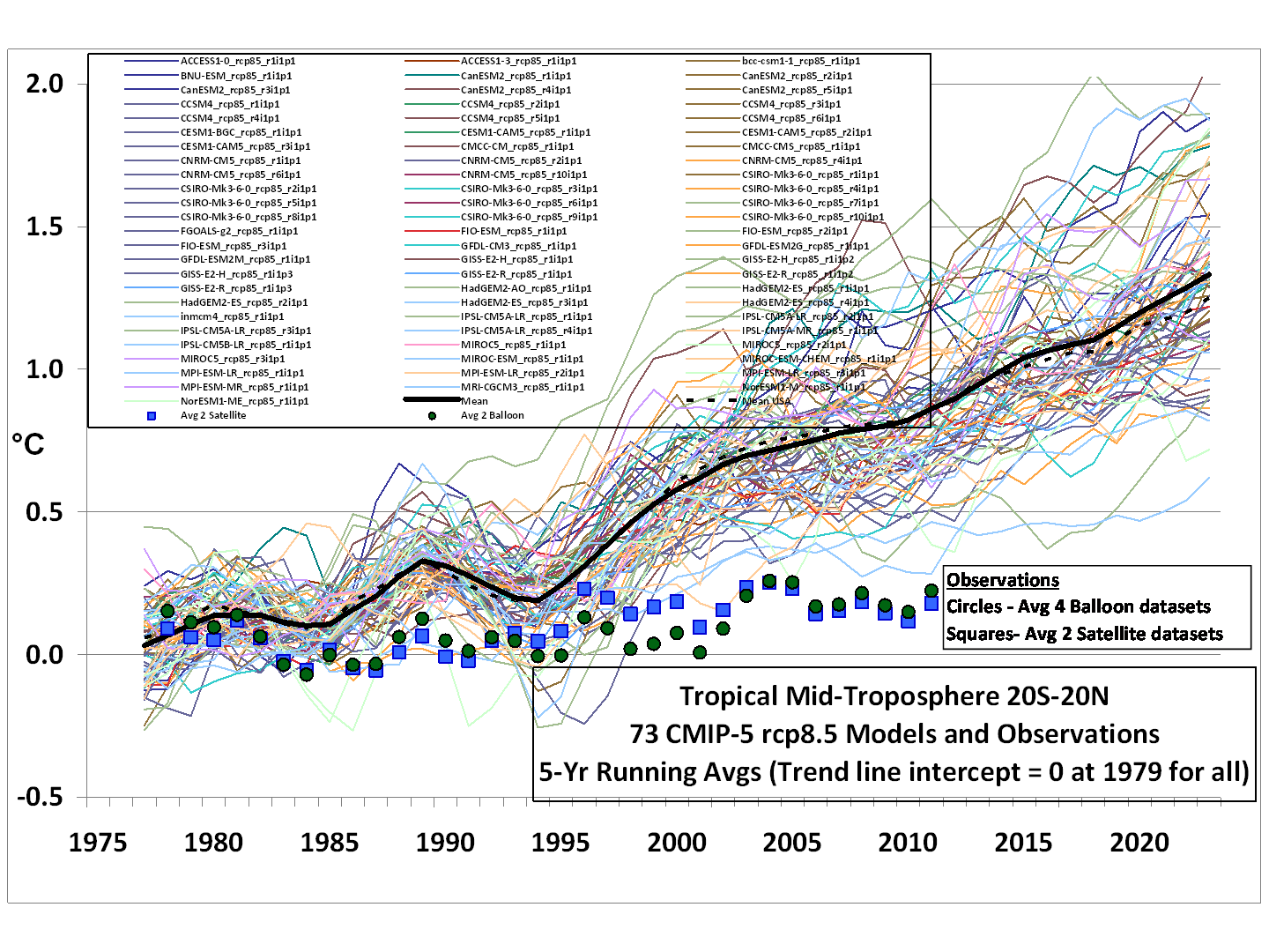
The MSU record has now been going for 34 years. Spencer has recently published a comparison between temperature predictions made by a large number of IPCC climate models and their projected future and the temperature record as shown by the MSUs and the balloons.
at http://www.drroyspencer.com/wp-content/uploads/CMIP5-73-models-vs-obs-20N-20S-MT-5-yr-means1.png
It is surely obvious that all the models are wrong and that their projections are nonsensical.
I might also add that the central line is also meaningless.
2. MURRY SALBY
Murry Salby is Professor of Climate Science at McQuarrie Univerity where he has an impressive research programme to be seen at
http://envsci.mq.edu.au/staff/ms/research.html
He has published a book “Physics of the Atmosphere and Climate”.
He has recently expounded his views on the climate in two Youtube presentations. I have found that it was necessary to see both of them several times before I got a clear idea of what he is claiming. The first one, at
was a presentation at the Sydney Institute on 2nd August 2011.
He begins by showing the paleo record based on ice cores and shows that there is a close correlation between carbon dioxide and temperature, with temperature coming first. The same applies to methane.
He then attaches it to the more recent CO2 record and plots the Carbon13 figures, which declined over the whole period. Since plant material prefers C12 this means that the additional CO2 comes from plant material. The IPCC claims that the additional plant material must come from combustion of fossil fuels, so this is their “Smoking Gun” that the increase in CO2 is caused by human-derived emissions.
But the extra plant-derived CO2 could be natural. Salby sets out to show that this is true. He shows a satellite map of natural sources of CO2 which come more from the tropics than from temperate regions (but only 6% more)
He then provides data and graphs which show that the additional CO2 results from what happens during a temperature fluctuation, using the satellite (MSU) temperature record since 1978. He shows that the CO2 which is released by a temperature increase is always greater than the CO2 absorbed when the temperature falls, providing a net increase in the atmosphere
The CO2 increase is from natural sources. It is not related to temperature, but to the behaviour of temperature fluctuations.
The second Youtube presentation at
took place at Hamburg 18th April 2013.
It starts with an attempt to clear up the discrepancy of the first presentation, where , carbon dioxide was related to temperature for the ice core proxies and where carbon dioxide was related to a difference between emissions and absorption during a temperature fluctuation for the recent measurements.
He does this by questioning the reliability of the ice core measurements, something that my late friend Zbigniew Jaborowski questioned in 1997.
He points out that the snow that traps air from the atmosphere and then solidifies irons out the fluctuations in temperature which are the real source of CO2 increase, and that some diffusion of the gases must happen when they are buried. By a rather elaborate set of mathematical calculations he restores the fluctuation effect from the ice cores and shows that it is compatible with his other calculations from recent measurements
He then extends his calculations of CO2 from temperature fluctuations by using the instrumental record. When he allows for its low reliability as you go back in the record (only 8% of the earth in 1860) he derives an impressive agreement between carbon dioxide increases and the calculated natural additions derived from temperature fluctuations over his entire range.
He shows that for the MSU record, carbon dioxide is completely unrelated to temperature,
We already know from the first part of this newsletter that climate models based on the assumption that carbon dioxide increases influence global temperature are fundamentally wrong so it does not matter much whether it comes from human-related emissions or from natural sources.
I vociferously object to science by Youtube. In the old days any new theory from a recognised academic would be welcomed by the journals, but nowadays any disagreement with the IPCC orthodoxy would have difficulty finding a place in a scientific journal.
All the same, this material from Salby needs to be properly documented before it could be considered seriously
Cheers
Vincent Gray
Wellington, New Zealand
Eli Rabett says:
“June 23, 2013 at 9:23 pm
Somewhat minor point, but Eli always thought that Spencer and Christy figured out how to use the MSU data considerably after the launch and were not the instrument scientists on the NOAA satellites that carried the MSUs.”
And the climate science world (you included?) first decided that it did not like the figures so produced, created another team to look at the same figures, and when they failed to come up with significantly different values, decided not to address why the two set of figures are different and continue to be different.
Bunnys obviously look at things differently.
Sorrry .Clarity required.
decided not to address why the two sets of land and satelliet figures are different and continue to be different.
After Wentz and Schnabel had shown that orbital decay was not properly handled by UAH, the climate scientists got the NAS to form an expert committee to look at the problem of why the surface records and UAH disagreed. Prabhakara did a nadir view analysis which indicated that there were problems with the UAH algoithms (nadir views being less subject to orbital decay problems). Go read the report from 2000 for details. Science as she is done. Live with it. However, to avoid boorishism, Eli will leave it there
So UAH and RRS are bad data and do not align with the nice thermometer record so they must by wrong. Still.
Need another carrot.
Bart says:
June 23, 2013 at 11:37 am
Bart, we have been there several times, but for the readers here again the arguments from my side (besides that there is no known natural physical or chemical process that can be the cause of the current increase).
Those portions with respond to anthropogenic forcing, indeed, which exist wholly in response to anthropogenic forcing, are in reality artificial sinks. They are created and maintained by anthropogenic inputs, and they would shrink away if anthropogenic inputs ceased.
This is a complete artificial separation: All sinks are natural, there are hardly any human sinks. These don’t respond to human inputs alone, they respond to every change in input, whatever its source. They don’t make a differentiation between human or volcanic or ocean or vegetation induced CO2. Thus there is nothing “artificial” to the increase in output from the atmosphere into the different reservoirs if the total amount of CO2 in the atmosphere increases, whatever its source. A 10% increase of CO2 due to humans or due to more ocean outgassing will have the same effect on the outputs.
Again for emphasis, this says NOTHING about the relative magnitudes of N and A.
The relative magnitudes of N and A are of not the slightest interest, as good as the relative magnitudes of turnover and gain of a factory are not of the utmost interest (they are, but the gain – or loss – is far more important than the turnover of capital).
As said several times before: if you bring 50 euro per day to you local bank branch without withdrawing any money and the net gain of that bank after a year is less than what you did bring in as capital, better look for another bank. No matter how big the investments and withdrawals of other clients were…
I still wonder how intelligent people don’t understand what every housewive with a minimum of budget control knows…
But let us look at the formula:
dC/dt= -a*C + N + A
First a real world problem: most of the sinks that absorb CO2 don’t respond to the total concentration of CO2 in the atmosphere, but to a difference in concentration with an equilibrium concentration. That is the case for plant growth which ceases completely below 180 ppmv for C3 plants and that is the case for the oceans, where no CO2 is absorbed or released when the temperature dependent pCO2 of the oceans is equal to the pCO2 in the atmosphere. That is less the case for rock weathering.
S0, the formula needs a zero carbon concentration where N and -a*C are in equilibrium and dC/dt = 0, without A. In the case of the oceans, even N(oceans) is dependent of the pCO2 difference between the ocean surface and the atmosphere. A fundamental point, as that is what happens if the CO2 concentration in the atmosphere increases: several of the sink fluxes increase and the main CO2 source flux from the oceans decreases.
Another problem is that both the oceans and vegetation are composed of fast en slow responses to changes of CO2 in the atmosphere: the ocean surface responds in 1-3 years, but only can react with some 10% of the change in the atmosphere (the Revelle factor) before a new equilibrium with the atmosphere is reached. The deep oceans have far more capacity, but their exchange with the atmosphere is far more limited and shows reponse times of around 50 years (and a turnover of many thousands of years…). The same applies to vegetation.
Thus the formula need some enhancement to reflect reality…
But let us show where the real world problem of any natural cause lies:
At least the basic formula needs to be changed to:
dC/dt= -a*(C – C0) + N + A
where C0 is temperature dependent and largely responsible for the small wiggles over the seasons (4-5 ppmv/°C) to the larger ones over the ice ages (8 ppmv/°C).
Some 50 years ago, the formula responded to (all in GtC and taking the current estimates for natural fluxes as base):
1.5 = a*(660-550) + 150 + 2.5
or a = 151/110 = 1.37
the overall net sink in natural fluxes in and out was 1 GtC/year
The human “contribution” to that sink is 0.66% according to the ratio human/natural carbon sinks.
The human “contribution” to the increase in the atmosphere was 100% according to the mass balance.
Assuming that the factor “a” didn’t change over time (the sinks respond linearly to CO2 concentration differences with the temperature dictated equilibrium), the current fluxes should be:
4.5 = 1.37*(840-550) + x + 9
or x = 402
the overall net sink in natural fluxes in and out is 4.5 GtC/year.
The human “contribution” to that sink is 1.1% according to the ratio human/natural carbon in the carbon sinks.
The human “contribution” to the increase in the atmosphere still is 100% according to the mass balance.
Again, it doesn’t matter that the natural fluxes increased a 2.7 fold over time (for which is not the slightest proof), as still the net natural contribution is negative in all cases, only the turnover increased a 2.7 fold…
Ferdinand Engelbeen says:
June 24, 2013 at 2:45 pm
“All sinks are natural, there are hardly any human sinks.”
Incorrect. Portions of the available sinks expand as a response to human inputs. That growth would not have occurred without human inputs. Therefore, that expansion has created an assortment of, in every sense of the word, artificial sinks.
“I still wonder how intelligent people don’t understand what every housewive with a minimum of budget control knows…”
Because housewives are generally not versed in feedback theory. If you are operating on the level of an ordinary housewife, that should be a clue to you that you do not understand the problem.
“First a real world problem: most of the sinks that absorb CO2 don’t respond to the total concentration of CO2 in the atmosphere, but to a difference in concentration with an equilibrium concentration.”
Trivial, as this is a linear system. Let Ceq be the equilibrium concentration. Then
d/dt(C – Ceq) = -a*(C – Ceq) + (N – a*Ceq) + A
Redefine Cd = C – Ceq, Nd – N-s*Ceq. Get
dCd/dt = -a*Cd + Nd + A
Now, you’re right back where you started from.
“At least the basic formula needs to be changed to:
dC/dt= -a*(C – C0) + N + A
where C0 is temperature dependent and largely responsible for the small wiggles over the seasons (4-5 ppmv/°C) to the larger ones over the ice ages (8 ppmv/°C).”
You’re just shuffling the deck chairs. Again, redifine Cd = C – C0, and you’re right back where we started. These manipulations are trivial, and simply obfuscating the problem.
“Some 50 years ago, the formula responded to (all in GtC and taking the current estimates for natural fluxes as base):
1.5 = a*(660-550) + 150 + 2.5”
What happened to the minus sign on “a”? If “a” is negative, you have positive feedback, and the system will diverge exponentially.
“Assuming that the factor “a” didn’t change over time (the sinks respond linearly to CO2 concentration differences with the temperature dictated equilibrium), the current fluxes should be:
4.5 = 1.37*(840-550) + x + 9
or x = 402
the overall net sink in natural fluxes in and out is 4.5 GtC/year.
The human “contribution” to that sink is 1.1% according to the ratio human/natural carbon in the carbon sinks.”
Even if you did not have the sign wrong, and your numbers were not all flaky, this is where you would have erred. Part of that 840 is due to the anthropogenic input over the years. You have to subtract that portion out before you actually get a measure of uniquely natural activity.
If you do not understand the elementary example I gave, you cannot hope to understand what is really going on, and you really should not be sticking your neck out so far.
What happened to the minus sign on “a”? If “a” is negative, you have positive feedback, and the system will diverge exponentially.
Rather, if “a” is positive.
Richard: So UAH and RRS are bad data and do not align with the nice thermometer record so they must by wrong. Still.
Actually at this point RSS and UAH align with GISS HadCRUT and NOAA very well thank you. Please do try and keep up.
“Rather, if “a” is positive.”
Which is to say, if “a” is negative in my original equation, you get positive feedback. Or, if you neglect the negative sign, as you appear to have done, and “a” is positive, you get positive feedback. In any case, you’ve got a positive feedback, and your equation diverges exponentially over time. It is basically an equation with all sources, and no sinks.
We ran through an example some time ago where we discussed putting hot and cold water in a sink, and I asked what temperature the water would eventually reach, given the input flow from one of the sources and the level of water that was reached. You agreed with me at that time that it depended entirely on the efficiency of the drain, i.e., the feedback factor, and I thought we had made a major breakthrough. But, then, with distance from that conversation, you fell back into your old habits, and now you are back to making your preposterous “mass-balance” claim.
Even explaining a trivial system as the one above, and how feedback negates your claim, I seem to make no headway. I don’t know what more I can do but continue pointing out you are wrong every time you bring it up. It is both very saddening and very frustrating, because it really is a freshman level problem, and there is no doubt about it.
Eli Rabett says:
June 24, 2013 at 5:50 pm
“Actually at this point RSS and UAH align with GISS HadCRUT and NOAA very well thank you.”
And, they all show that temperature is driving CO2 very well, thank you.
“””””””…….Bart says:
June 24, 2013 at 5:22 pm
Ferdinand Engelbeen says:
June 24, 2013 at 2:45 pm
“All sinks are natural, there are hardly any human sinks.”….”””””
I disagree. While old growth forests are carbon neutral. tree farming; aka agriculture projects are carbon sinks.
New Zealand has some of the larges agricultural forests in the world (maybe the largest) making NZ a carbon sink. The largest ( well the only large) land carbon sink on the planet, is North America. Well more specifically the USA. Canada would be part of this, if it were not so cold with a short growing season.
Agriculture and tree farming make it so.
If global Temperatures rose lengthening the Canada growing season, North America would be an even bigger carbon sink.
All other continents are either carbon sources (Australia) or carbon neutral.
Australia is not to blame; nothing grows there.
george e. smith says:
June 24, 2013 at 7:29 pm
“While old growth forests are carbon neutral. tree farming; aka agriculture projects are carbon sinks.”
Yes, but these are not the category of artificial sinks we are looking for, and they are a small part of the overall budget.
We are looking for sinks whose growth is fueled by the ready availability of anthropogenically released CO2. We send CO2 up in the air, and most of it settles back down, initiating biological and mineral processes which increase their activity based on the availability of CO2.
Had we not released that CO2, those processes would not have been initiated. So, in a very real sense, we created those additional sinks. They are artificial sinks.
This is the problem with the “mass balance” argument. It is not true that all significant sinks are strictly natural. If they would not have come into being without our activity, then they are artificial, as much as an airplane or a truck or a toxic waste dump is artificial, because we engaged in activities which brought them into being.
An automobile is made of iron, steel, aluminum, leather, glass, etc. It is, in fact, 100% natural content. Yet, surely an automobile is an artificial construct? Surely nobody would claim that automobiles are natural? Yet, this is precisely what Ferdinand et al., are claiming, that something which we created out of natural materials is necessarily “natural”.
An example to attempt further clarification: suppose we pump an excess of CO2 into a greenhouse. What happens? The plants grow more rapidly and to greater size, incorporating that extra carbon into their structure. They have much more carbon in them their normal, scrawny counterparts subjected to normal atmospheric levels of CO2. They sank the carbon we provided them. There is no way anyone could claim that, left to grow naturally, they would have stored that much carbon away. They are artificial carbon sinks. Wholly natural in material, yet artificial sinks nevertheless.
Bart says:
June 24, 2013 at 5:24 pm
What happened to the minus sign on “a”? If “a” is negative, you have positive feedback, and the system will diverge exponentially.
Sorry, my mistake, of course it must be -a where -a*(C – C0) and N nearly compensate each other, -a*(C-C0) being slightly larger than N. The rest of the calculation still is the same, taking into account the change in sign.
Anyway, in all cases the “expansion” of the sinks due to human emissions is negligible and near all sink capacity is natural.
george e. smith says:
June 24, 2013 at 7:29 pm
I disagree. While old growth forests are carbon neutral. tree farming; aka agriculture projects are carbon sinks.
Not quite right: most of what is farmed sooner or later is recycled into CO2 back into the atmosphere, directly by burning or indirectly as human and animal, insect or bacterial food. As more land use change is destroying forests in the tropics than is extra planted in other countries, the estimates are some 1 GtC/year extra CO2 releases from human activities in land use.
I don’t use that in any calculation, as these figures are way to uncertain compared to the fossil fuel budget and only are additional to that.
Eli Rabett says:
June 24, 2013 at 5:50 pm
“Richard: So UAH and RRS are bad data and do not align with the nice thermometer record so they must by wrong. Still.
Actually at this point RSS and UAH align with GISS HadCRUT and NOAA very well thank you. Please do try and keep up.”
Please. They most cfertainly do not agree that any particular rate of change being the same!
Try this for a satellite referenced historical data series.
http://www.woodfortrees.org/plot/best/offset:-0.4/scale:0.5/plot/hadcrut4gl/offset:-0.16/scale:0.86/plot/rss/plot/uah/offset:0.1
Have another carrot and think first 🙂
Bart says:
June 24, 2013 at 5:22 pm
Trivial, as this is a linear system. Let Ceq be the equilibrium concentration. Then
d/dt(C – Ceq) = -a*(C – Ceq) + (N – a*Ceq) + A
Sorry, that is already two steps too far.
The sinks react on C-Ceq that is on total C, not on individual emissions. In first instance the natural and human increases are additional to the total carbon in the atmosphere:
d/dt(C’ – Ceq) = -a*(C’ – Ceq) + N + A
Where C’ = C + N + A
The sinks don’t make a differentiation between CO2 already in the atmosphere, whatever its source, or the additional CO2 from natural or human origin.
Further, this is a huge simplification of what happens in nature: There are fast processes at work and slow processes. The bulk of the CO2 movements is over the seasons, reacting very fast on temperature changes.
Most of the CO2 movement in plants is the growing and decay of leaves and small stems. That budget is nearly in equilibrium for tropical forests, but largely seasonal in growth and decay for the mid and high latitude forests.
In spring when a lot of leaves are growing, the bulk of the CO2 transfer of about 60 GtC is used. That can be seen in the -4 to -10 ppmv drop for the NH in the Mauna Loa to Barrow CO2 levels:
http://www.ferdinand-engelbeen.be/klimaat/klim_img/month_2002_2004_4s.jpg
Mauna Loa only lags Barrow, because of the time needed to redistribute the CO2 levels to higher altitudes. The SH has less variability due to less vegetation compared to the ocean area.
The growth and decay of leaves is a fast process: growth in a few months and decay in months to a few years, with a small part remaining for very long times (humus, peat, browncoal, coal). The growth and decay of leaves is responding fast to fast temperature (and moisture) changes, hardly influenced by long term temperature changes, but the slower processes are influenced. That is the carbon budget of what remains in the soils as roots, peat and other slow or near non-degrading carbon. That budget is known from the oxygen balance: from slightly negative to near zero before 1990 to slightly positive since the 1990’s. The world is “greening”. That process is influenced by long-term temperature changes (mostly on very long term, by adding suitable land at the expense of ice fields and permafrost), but far more important by atmospheric CO2 pressure.
The difference: the 60 GtC in and output from plants is mostly seasonal up to a few years, but the long-term budget is currently an extra storage of carbon of about 1 GtC/year for the whole biosphere, largely atmospheric CO2 pressure related, hardly temperature dependent.
The same for the carbon budget of the oceans:
All CO2 releases and uptakes by the oceans are pressure related. Without a partial pressure difference between the atmosphere and the oceans, there is no CO2 transfer. Of course temperature influences the pCO2 of the oceans to some extent, but that is not more than 16 ppmv/°C, according to Henry’s Law.
Here again, most of the transfer is seasonal: 50 GtC out of the ocean surfaces in summer, 51 GtC into the ocean surfaces in winter, mostly in the mid-latitudes.
Part of the transfer is continuous: 40 GtC/year out of the ocean upwellings near the warm equator waters, 42 GtC/year into the cold polar waters and going down into the deep ocean layers.
Any changes in temperature will have a fast response (1-3 years) in the surface layer for 10% of the change in the atmosphere (the Revelle factor), but a slower response on the deep oceans circulation.
Thus at least you need to split your formula in fast responses and slow responses.
Further, as the main CO2 fluxes between the biosphere and the atmosphere at one side and of the oceans and the atmosphere at the other side work countercurrent for temperature changes, the real global N in the above formula is only ~10 GtC for a global seasonal change of ~1°C in temperature. Thus of the same magnitude as the yearly human contribution… Makes a lot of difference in the budgets…
Bart says:
June 24, 2013 at 10:39 pm
We are looking for sinks whose growth is fueled by the ready availability of anthropogenically released CO2.
Either the contribution of human releases to the increase is trivial and so is the human contribution to the increase in total sinks, or human releases are responsible for the bulk of the increase in the atmosphere and thus responsible for the bulk of the increase in sink capacity, which for the fast processes still is only 3% of the total fluxes in and out of the atmosphere…
There are no sink processes that react extra on anthro CO2 releases only. All sink processes react on total CO2 and/or temperature. Pure theoretical, the total CO2 concentration near human sources can be increased near land plants, but that is mostly at night, when land plants are net sources of CO2, especially under inversion and low wind conditions. During the day, there is far more turbulence, effectively mixing the surface air layers with the rest of the atmosphere.
I have tried to follow Murry Salby’s lecture in Hamburg in detail (while travelling, could only pick up a few items).
Where he goes wrong, is on following points:
At about 11 minutes, he interpretes the covariability between temperature variations and CO2 variations. While there is a huge covariability between the two, where it goes wrong is that he starts to integrate that over time, assuming a continuous CO2 flow for a sustained temperature difference against an arbitrary baseline. The same error that Bart makes in his interpretation.
There is a real correlation between temperature changes and CO2 changes of between 4-8 ppmv/°C over short to very long time frames. But there is no continuous change of CO2 levels if the temperature remains on a continuous high (or low) level above (or below) an arbitrary baseline.
That is quite visible in the ice core record: The covariability is quite high at about 8 ppmv/°C, but when the temperature starts to increase from the depth of the glacial period, the total time needed to reach some 12°C increase is some 5000 years and shows an increase of 100 ppmv over that period. That is integrated over the whole period in average 0.02 ppmv/year (all data based on the Vostok ice core for the period 135-130 kyr BP):
http://www.ferdinand-engelbeen.be/klimaat/klim_img/eemian.gif
The current increase in CO2 shows a covariation of 4-5 ppmv/°C for time frames of seasons to a few years. But should give over 100 ppmv/°C over a period of 50 years, or average over 2 ppmv/year, 100 times higher than during the glacial-interglacial transition, according to Salby and Bart. Further, the average 2°C higher than today temperatures over the previous interglacial remained higher over thousands of years, without any measureable influence on CO2 levels.
The main misinterpretation by Salby and Bart is that temperature is seen as the only driving variable, without influence from the CO2 increase/decrease on the CO2 fluxes. In the past, temperature indeed was the only driving variable, but the CO2 changes did bring the CO2 fluxes back to equilibrium after each temperature change, even if that did take 800 years or more. Nowadays, temperature is not the only driving variable and all what the temperature variability does is modulating the sink rate of the increase in CO2 of the atmosphere, with only a small increase in CO2 due to higher temperatures since the LIA…
—————
Where Salby again goes wrong is at about 17 minutes where he uses the Conservation Equation:
dr/dt = gT – ar
where g(amma) is the change rate in CO2 caused by temperature and a(lpha) the time scale of damping.
First, damping goes two ways out, so the – ar becomes + ar when temperature (and CO2 levels) go down.
Second, of course, the time scale of damping is important to know if fast changes would be noticed or not, as damping does flatten the CO2 record, but in no way changes the average CO2 levels over the period that is damped.
His misinterpretation is confirmed a little further, where he compares the removal of CO2 in ice cores (by damping) to the removal of CO2 by plants, but there is no such mechanism at work in ice cores. To the contrary, the Greenland ice cores suffer from the opposite, due to Icelandic volcanic deposits…
Even taking into account the different resolutions of different ice cores, a similar as current increase in CO2 levels would be measurable in every ice core, including even in the ~600 year resolution of the Vostok ice core, but certainly over the past 70,000 years, where we have ice cores with a resolution of 40 years and less…
More later on, when I have listened further…
Further on Salby (quite difficult to follow by times):
After 17 minutes, he shows the increase of plant growth as result of increased CO2. That indeed happened, but is quite limited. Before 1990, there might have been a net contribution of CO2 from the total biosphere of about 0.5 GtC/year, after 1990 the biosphere is an increasing sink of about 1 GtC/year. Thus a difference of 1.5 GtC/year for an increase of some 140 GtC (70 ppmv) over the past 50 years in the atmosphere. Not negligible, but not the main sink of CO2, as other necessities are the limiting factors for plant growth.
Further, not applicable to marine biology, where CO2 is not the limiting factor at all.
After 25 minutes, he compares the amplitude of real variances in the atmosphere with the measured variance in ice cores for different frequencies. If I do understand his interpretation well, the higher the frequency in the atmospheric change, the better the variances in the ice cores reflect the variances in the atmosphere??? As far as I know, it is just the opposite, that even any full cycle with a cycle length less than the resolution would be invisible in the ice record and the longer the cycle length, the better it is conserved in the ice record…
Further on he has lost all sight on reality, as he says that the CO2 levels at longer times scales may be more underestimated than on shorter time scales. As example he gives that on a timescale of 10 kyr the ice core underestimates the variance of the atmosphere with a factor 2, making that a 20 ppmv peak and drop of CO2 in the atmosphere would only give a 4 ppmv variability in the ice core. Worse on a timescale of 100 kyr: a variance of 1000 ppmv in the atmosphere would only be seen as a 100 ppmv variance in the ice core.
That is without taking into account all the different resolutions of the different ice cores. Sorry, but that is a serious misinterpretation of what the distribution of CO2 variations in ice cores do.
Then after 30 minutes he looks at the suppressing of high frequency variations in the ice core. Again, while that is true, that highly depends of the resolution of the ice core in combination with the frequency of the variations, but his interpretation of a 10 fold suppression on time scales of 10 kyrs is completely out of reality for the higher resolution ice cores like Taylor Dome (~40 years over 70 kyears).
That all is based on some estimate of a huge CO2 migration in ice (shown after 32 minutes) which is not measured in any ice core. If that would be the case, the ice core CO2 record in the far past would get flatter and flatter for every interglacial back in time, which is not measured at all: the CO2/temperature ratio remains the same for all glaciations/deglaciations over 800 kyears.
I have the impression that Salby simply uses any possible interpretation to fit the equations from past and present, even if that is completely out of reality…
Further on Salby… part 3.
The interpretation of the 13C reduction over time since about 1850 at about 37 minutes is wrong. There are few sources of low 13C on earth, mostly recent organics and fossil organics. Even releasing some (abiotic or not) methane from the earth’s mantle or from permafrost would be noticed in the CH4 record, which is essentially flat over the past decades (but still a lot higher than in the previous interglacial).
From the two main sources, we know that the current biosphere is a net absorber of CO2 thus all what is left is the human emissions which are a threefold of what is needed to reduce the observed 13C level of the atmosphere, the other 2/3rd is mixed into the (deep) oceans over time…
At 43 minutes, his interpretation of the response of the CO2 increase rate to increased temperature is that the natural sources increased. But as the human emissions were always larger than the increase in the atmosphere, the right interpretation is that the net sink rate of the natural cycle decreased…
The same misinterpretation in the 13C record: when CO2 increases more during a year, d13C levels go more down. His interpretation is that less high 13CO2 is released (by natural sources), while total emissions increased (?), while in fact less human low 13CO2 is absorbed…
Where it completely goes wrong is at 47 minutes where he starts the integration of the temperature/moisture effect on the rate of change of CO2 levels from 1982-2007 above an completely arbitrary baseline of 0.3 ppmv/yr. That is curve fitting, not based on any physical explanation of what happens in reality. Again, there is no source on earth that delivers a constant amount of CO2 to the atmosphere for a sustained difference in temperature of a few tenths of a degree without being counteracted by some pressure dependent CO2 flows for the change in atmospheric CO2…
Too many problems with the interpretation from Salby…
There it ends for me (for the moment).
Ferdinand Engelbeen says:
June 25, 2013 at 12:11 am
“Anyway, in all cases the “expansion” of the sinks due to human emissions is negligible and near all sink capacity is natural.”
Mere assertion on your part, with no supporting evidence whatsoever. The temperature-CO2 relationship shows you are wrong.
FerdiEgb says:
June 25, 2013 at 1:36 am
“Further, this is a huge simplification of what happens in nature:”
I stated this in the first sentence of the example. It does not matter. Feedback acts in the same way regardless. You are not taking account of the influence of the anthropogenic output on the “natural” sinks, and you are including artificially driven components in the “natural” column for your accounting.
“Most of the CO2 movement in plants is the growing and decay of leaves and small stems. That budget is nearly in equilibrium for tropical forests, but largely seasonal in growth and decay for the mid and high latitude forests.”
Incorrect. When the forest expands, that carbon is sunk. It is not “unsunk” until the forest returns to its former size.
“Thus at least you need to split your formula in fast responses and slow responses.”
No. I have given an explicit counterexample to your “mass-balance” methodlogy. It does not matter how the actual system behaves. The principle is the same. You are not taking account of the influence of the anthropogenic output on the “natural” sinks, and you are including artificially driven components in the “natural” column for your accounting.
FerdiEgb says:
June 25, 2013 at 2:08 am
“There are no sink processes that react extra on anthro CO2 releases only.”
And, conversely, there are no sink processes which “react extra” on natural releases only. The anthropogenic releases induce sink expansion. Those portions of the sinks which expand due to human production are artificial sinks.
FerdiEgb says:
June 25, 2013 at 5:35 am
“Where he goes wrong, is on following points:”
You’re a nice guy, Ferdinand, but I must say, it displays a lot of gall for you to take on as accomplished a fellow as Dr. Salby when you apparently cannot even solve a simple, first order, ordinary differential equation and draw the appropriate conclusions.
“But there is no continuous change of CO2 levels if the temperature remains on a continuous high (or low) level above (or below) an arbitrary baseline.”
Yes, there is. It is evident in the near perfect correlation between integrated temperatures and CO2. It comes about because there is a continuous flow, and a temperature dependent pumping of CO2 into the atmosphere. An imbalance, for instance, in the CO2 concentration of upwelling and downwelling waters is a continuous CO2 pump, into the atmosphere if the former exceeds the latter.
“That is quite visible in the ice core record:”
The relationship is evident, and Salby went into much detail about how it comes about, and how it is consistent with the integral relationship. The mathematics are complicated, but straightforward to a control systems engineer, and irrefutable.
FerdiEgb says:
June 25, 2013 at 7:15 am
“Before 1990, there might have been a net contribution of CO2 from the total biosphere of about 0.5 GtC/year, after 1990 the biosphere is an increasing sink of about 1 GtC/year. “
This is all circular reasoning. Your numbers are based on the very presumption you are trying to establish.
FerdiEgb says:
June 25, 2013 at 8:23 am
More circular reasoning.
I do not want to be getting into these tortured interpretations with you at this time. I merely want to establish that your “mass-balance” argument is not compelling evidence in favor of human responsibility for the observed increase in CO2 over the last century. Once we have established this, we can move on to other things.
Bart,
All I have seen from you and Salby, is a pure theoretical solution which is possible, but not probable.
Not probable, as the theoretical possibility violates several observations. These observations are either ignored or downplayed, both by you and Salby, because they don’t fit the theory.
Take e.g. what Salby says about ice cores. Both the long term and short term variancies are underestimated in ice cores, compared to what happened in the atmosphere, accoring to him. That the long term variances are underestimated can’t be right in any way and short term variance suppression is merely a matter of resolution, which widely differs between different ice cores. That is completely ignored by Salby.
Further, the examples he does give are one-sided: any peak of 1000 ppmv over 100 kyrs only shows a 100 ppmv peak in the ice core, according to his theory. But what he forgets to tell is that any drop of 100 ppmv in the ice core then would represent a drop of 1000 ppmv in the atmosphere. That is below zero… Ice cores do filter the fast changes, but they don’t change the average over the resolution period.
That all was based on his own estimate of huge migration of CO2 in the ice cores, which in reality is so low that it is practically unmeasurable.
About your examples. Let us assume that the natural sources (your ocean upwelling) really increased in such a way that it is the main cause of the increase in the atmosphere and dwarf the human contribution, thanks to a fast response of the sinks (no matter the relative contribution).
As there is a huge difference in 13C/12C ratio between ocean CO2 and fossil fuel CO2, it is easy to track the evolution of the changes in fluxes, as d13C levels were regularly measured since about 1978, before that in ice cores.
Here my own estimate of the deep ocean exchanges, based on a fixed exchange between deep oceans and the atmosphere:
http://www.ferdinand-engelbeen.be/klimaat/klim_img/deep_ocean_air_zero.jpg
The main difference between the theoretical drop in d13C from fossil fuel burning and the real drop is from the deep ocean exchange. Low d13C is going into the deep and high d13C is coming out of the deep.
The ocean surface exchange is two ways and hardly plays a role and vegetation too is largely two ways but permanent storage and/or more decay may give an unbalance, which may be the cause of the mismatch before 1960.
Now, if we may assume that the deep ocean emissions (and sinks) increased from about 40 GtC in 1960 to 400 GtC in 2010 (all other fluxes remaining constant) that would give following trend of d13C in the atmosphere (assuming no change before 1960):
http://www.ferdinand-engelbeen.be/klimaat/klim_img/deep_ocean_air_increase.jpg
Thus any huge increase of the deep ocean circulation (no matter if that is only exchange or additional) would reduce the 13C/12C ratio in the atmosphere, despite the additional low 13CO2 from fossil fuel burning. Which is not observed.
Conclusion: there is no substantial increase of deep ocean CO2 upwelling.
That is only one of the several observations that are violated by the theoretical natural increase of CO2 over the past 50 years… Thus in my opinion, the theory is invalidated…
Incorrect. When the forest expands, that carbon is sunk. It is not “unsunk” until the forest returns to its former size.
Any extra CO2 sink or release from the total biosphere can be measured as the difference between calculated oxygen use from fossil fuel burning and the measured oxygen use in the atmosphere. Since about 1990, the oxygen use shows a net absorption of ~1 GtC/year by the biosphere. Before 1990 they are estimated based on the deviation of the 13C/12C balance as shown in the d13C trends above. See further:
http://www.bowdoin.edu/~mbattle/papers_posters_and_talks/BenderGBC2005.pdf
Ferdinand Engelbeen says:
June 26, 2013 at 3:46 am
Now, if we may assume that the deep ocean emissions (and sinks) increased from about 40 GtC in 1960 to 400 GtC in 2010 (all other fluxes remaining constant)
I made an error, as the fluxes in and out of the atmosphere may have increased from to 400 GtC over a year, but that is for all fluxes together. If the non-deep ocean fluxes remained the same, then the deep ocean fluxes had to grow from 40 GtC/year to 290 GtC/year, not to 400 GtC/year. That gives the following trend in d13C, compared to fixed deep ocean fluxes:
http://www.ferdinand-engelbeen.be/klimaat/klim_img/deep_ocean_air_increase_290.jpg
The only difference with the 40-400 GtC/year increase is that the recovery from the low 13C human contribution is slower.
Ferdinand Engelbeen says:
June 26, 2013 at 3:46 am
“All I have seen from you and Salby, is a pure theoretical solution which is possible, but not probable.”
I understand that it is difficult for a lay person to understand why it the necessary conclusion. I do not hold out much hope that it will be widely accepted until the observations begin to show a marked divergence in emissions and measured concentration. This has already begun, so I think all we have to do is wait and have patience.
My main goal right now, though, is to get you to understand how and why the “mass balance” argument is flawed, and to stop promoting it, perhaps even to actively oppose it when you see others doing so. Every other argument on your list is subject to debate, but the “mass-balance” argument, were it legitimate, would be decisive. It would be the only argument one needed to know, and there would be no alternative possibility.
It is not legitimate. In a system in which sinks expand in response to all forcings, part of their inventory is going to be artificially induced, and cannot be accounted strictly in the “natural” column.