UPDATE: I’ve added graphs of the difference between the observations and the models at the end of the post, under the heading of DIFFERENCE.
####
We’ve shown in numerous posts how poorly climate models simulate observed changes in temperature and precipitation. The models prepared for the upcoming Intergovernmental Panel on Climate Change (IPCC) 5th Assessment Report (AR5) can’t simulate observed trends in:
1. satellite-era sea surface temperatures globally or on ocean-basin bases,
2. global satellite-era precipitation,
3. global, hemispheric and regional land surface air temperatures, and
In this post, we’ll compare the multi-model ensemble mean of the CMIP5-archived models, which were prepared for the IPCC’s upcoming AR5, and the new GISS Land-Ocean Temperature Index (LOTI) data. As you’ll recall, GISS recently switched sea surface temperature datasets for their LOTI product.
We have not presented trend maps in earlier comparisons of observed and modeled global land plus sea surface temperature anomalies, so, for the sake of discussion, we’ll provide them with this post. A comparison is shown in Figure 1 for the period of 1880 to 2012. 
Figure 1
The maps in Figure 1 show the modeled and observed linear trends for the full term of the GISS data, from 1880 to 2012. The CMIP5-archived simulations indicate stronger-than-observed polar-amplified warming at high latitudes in the Northern Hemisphere. The models also show a more uniform warming of the tropical Pacific, while the observations show little warming. There are a number of other regional modeling problems.
Presenting the trends over the full term of the GISS data actually tends to make the models look as though they perform reasonably well. But when we break the observations and model outputs into the 4 periods shown in Figure 2, the models do not fare as well. In fact, the trend maps will help to show how poorly the models simulate observed temperature trends during the early cooling period (1880 to 1917), the early warming period (1917 to 1944), the mid-20th century flat temperature period (1944 to 1976) and the late warming period (1976 to 2012).

Figure 2
To head off complaints by global warming enthusiasts, the IPCC acknowledges those warming and cooling (flat temperature) periods in their 4th Assessment Report. As a reference, see Chapter 3 Observations: Surface and Atmospheric Climate Change of the IPCC’s AR4. Under the heading of “3.2.2.5 Consistency between Land and Ocean Surface Temperature Changes”, the IPCC states with respect to the surface temperature variations over the period of 1901 to 2005 (page 235):
Clearly, the changes are not linear and can also be characterized as level prior to about 1915, a warming to about 1945, leveling out or even a slight decrease until the 1970s, and a fairly linear upward trend since then (Figure 3.6 and FAQ 3.1).
You’ll notice by extending the data back to 1880, the data shows a cooling trend before 1917.
A NOTE ABOUT THE USE OF THE MODEL MEAN
The following discussion is a reprint from the post Blog Memo to John Hockenberry Regarding PBS Report “Climate of Doubt”.
The model mean provides the best representation of the manmade greenhouse gas-driven scenario—not the individual model runs, which contain noise created by the models. For this, I’ll provide two references:
The first is a comment made by Gavin Schmidt (climatologist and climate modeler at the NASA Goddard Institute for Space Studies—GISS). He is one of the contributors to the website RealClimate. The following quotes are from the thread of the RealClimate post Decadal predictions. At comment 49, dated 30 Sep 2009 at 6:18 AM, a blogger posed this question:
If a single simulation is not a good predictor of reality how can the average of many simulations, each of which is a poor predictor of reality, be a better predictor, or indeed claim to have any residual of reality?
Gavin Schmidt replied with a general discussion of models:
Any single realisation can be thought of as being made up of two components – a forced signal and a random realisation of the internal variability (‘noise’). By definition the random component will uncorrelated across different realisations and when you average together many examples you get the forced component (i.e. the ensemble mean).
To paraphrase Gavin Schmidt, we’re not interested in the random component (noise) inherent in the individual simulations; we’re interested in the forced component, which represents the modeler’s best guess of the effects of manmade greenhouse gases on the variable being simulated.
The quote by Gavin Schmidt is supported by a similar statement from the National Center for Atmospheric Research (NCAR). I’ve quoted the following in numerous blog posts and in my recently published ebook. Sometime over the past few months, NCAR elected to remove that educational webpage from its website. Luckily the Wayback Machine has a copy. NCAR wrote on that FAQ webpage that had been part of an introductory discussion about climate models (my boldface):
Averaging over a multi-member ensemble of model climate runs gives a measure of the average model response to the forcings imposed on the model. Unless you are interested in a particular ensemble member where the initial conditions make a difference in your work, averaging of several ensemble members will give you best representation of a scenario.
In summary, we are definitely not interested in the models’ internally created noise, and we are not interested in the results of individual responses of ensemble members to initial conditions. So, in the graphs, we exclude the visual noise of the individual ensemble members and present only the model mean, because the model mean is the best representation of how the models are programmed and tuned to respond to manmade greenhouse gases.
In other words, IF (big if) global surface temperatures were warmed by manmade greenhouse gases, the model mean presents how those surface temperatures would have warmed.
Let’s start with the time period when the models perform best, the recent warming period. And we’ll work our way back in time.
NOTES: For the trend maps in Figures 4, 6, 8 and 10, I’ve used a different range for the contour levels than those used in Figure 1. The contour range is now -0.05 to +0.05 deg C/year to accommodate the higher short-term trends. And for the temperature anomaly comparisons, I used the base period of 1961-1990 for anomalies. Those are the base years used by the IPCC in their model-data comparisons in Figure 10.1 from the Second Order Draft of AR5.
RECENT WARMING PERIOD – 1976 TO 2012
Figure 3 compares the observed and modeled linear trends in global land plus sea surface temperature anomalies for the period of 1976 to 2012. The models have overestimated the warming by about 28%. The divergence between the models and the data in recent years is evident. It’s no wonder James Hansen, now retired from GISS, used to hope for another super El Niño.

Figure 3
Figure 4 compares the modeled and observed surface temperature trend maps for 1976 to 2012. The models show warming for all of the East Pacific, while the data indicates little warming to cooling there. For the western and central longitudes of the Pacific, the models fail to show the ENSO-related warming of the Kuroshio-Oyashio Extension (KOE) east of Japan and the warming in the South Pacific Convergence Zone (SPCZ) east of Australia. The models also underestimate the warming in the mid-to-high latitudes of the North Atlantic. Modeled land surface temperature anomaly trends also show very limited abilities on regional bases, but that’s not surprising since the models simulate the sea surface temperature trends so poorly.

Figure 4
MID-20th CENTURY FLAT TEMPERATURE PERIOD
If we were to look only at the linear trends in the time-series graph, Figure 5, the modeled trend is not too far from the observed trend, only 0.026 deg C/decade.

Figure 5
However, as discussed in the post Polar Amplification: Observations versus IPCC Climate Models, the climate models fail to present the polar amplified cooling that existed during this period. See Figure 6. (Yes, polar-amplified cooling exists in the Arctic during cooling periods, too.) The climate models failed to simulate the cooling at high latitudes of the North Pacific and in the mid-to-high latitudes of the North Atlantic. The climate models also failed to simulate the warming of sea surface temperatures in the Southern Hemisphere, and they missed the warming of Antarctica.

Figure 6
EARLY WARMING PERIOD – 1917 TO 1944
Atrocious, horrible and horrendous are words that could be used to describe the performance of the CMIP5-archived climate models during the early warming period of 1917 to 1944. See Figure 7. According to the models, if greenhouse gases were responsible for global warming, global surface temperatures should only have warmed at a rate of about +0.049 deg C/decade. BUT according to the new and improved GISS Land-Ocean Temperature Index (LOTI) data, global surface temperatures warmed at a rate that was approximately 3.4 times faster or about 0.166 deg C/decade. That difference presents a number of problems for the hypothesis of human-induced, greenhouse gas-driven global warming, which we’ll discuss later in this post.

Figure 7
Looking at the maps of modeled and observed trends, the models failed to simulate the general warming of sea surface temperatures from 1917 to 1944 and they failed to capture the polar amplified warming at high latitudes of the Northern Hemisphere. As discussed in the post about polar amplification that was linked earlier, the observed warming rates at high latitudes of the Northern Hemisphere were comparable during the early and late warming periods (See the graph here).

Figure 8
Note: Areas in white in the GISS map have no data or they don’t have sufficient data to perform the trend analyses, which I believe is a threshold of 50% in the KNMI Climate Explorer.
EARLY COOLING PERIOD – 1880 TO 1917
If the data back this far in time is to be believed (that’s for you to decide), surface temperatures cooled, Figure 9, but the model simulations show they should have warmed slightly.

Figure 9
The observations-based map in Figure 10 shows land and sea surface temperature trends seeming to be out of synch during this period—sea surface temperatures show cooling while land surface temperatures show warming in many areas.

Figure 10
If GISS had kept HADISST as their sea surface temperature dataset for this period, the disparity between land and ocean trends would not have been as great. That is, the HADISST data they formerly used does not show that much cooling during this period.
A MAJOR FLAW IN THE HYPOTHESIS ON HUMAN-INDUCED GLOBAL WARMING
The observed warming rate during the early warming period is comparable to the trend during the recent warming period. See Figure 11.

Figure 11
But according to the models, Figure 12, if global temperatures were warmed by greenhouse gases, global surface temperatures during the recent warming period should have warmed at a rate that’s more than 4 times faster than the early warming period—or, more realistically, the early warming period should have warmed at a rate that’s 22% of the rate of the late warming period—yet the observed warming rates are comparable.

Figure 12
That’s one of the inconsistencies with the hypothesis that anthropogenic forcings are the dominant cause of the warming of global surface temperatures over the 20th Century. The failure of the models to hindcast the early rise in global surface temperatures illustrates that global surface temperatures are capable of warming without the natural and anthropogenic forcings used as inputs to the climate models.
Another way to look at it: the data also indicate that the much higher anthropogenic forcings during the latter later warming period compared to the early warming period had little to no impact on the rate at which observed temperatures warmed. In other words, the climate models do not support the hypothesis of anthropogenic forcing-driven global warming; they contradict it.
THE OTHER MAJOR FLAW IN THE HYPOTHESIS ON HUMAN-INDUCED GLOBAL WARMING
Ocean heat content data since 1955 and the satellite-era sea surface temperatures indicate the oceans warmed naturally. Refer to the illustrated essay “The Manmade Global Warming Challenge” (42mb).
CLOSING
Climate models cannot simulate the observed rate of warming of global land air plus sea surface temperatures during the early warming period (1917-1944), which warmed at about the same rate as the recent warming period (1976-2012). The fact that the models simulate the warming better during the recent warming period does not indicate that manmade greenhouse gases were responsible for the warming—it only indicates the models were tuned to perform better during the recent warming period.
The public should have little confidence in climate models, yet we are bombarded by the mainstream media almost daily with climate model-based conjecture and weather-related fairytales. Climate models have shown little to no ability to reproduce observed rates of warming and cooling of global temperatures over the term of the GISS Land Ocean Temperature Index. The IPCC clearly overstates its confidence in model simulations of the climate variable most commonly used to present the supposition of human-induced global warming (e.g., surface temperature). After several decades of development, models continue to show no skill at establishing that global warming is a response to increasing greenhouse gases. No skill whatsoever.
SOURCE
The GISS LOTI data and the outputs of the CMIP5-archived models are available through the KNMI Climate Explorer.
UPDATE 1
DIFFERENCE
The difference between the GISS land-ocean temperature index data and the CMIP5 multi-model mean (Data Minus Model) is shown in Figure Supplement 1. The recent divergence of the models from observations has not yet reached the maximum differences that exist toward the beginning of the data—maybe in a few more years.

Figure Supplement 1
The differences do of course depend on the base years used for anomalies. As noted in the post, I’ve used the base years of 1961-1990 to be consistent with the base period used by the IPCC in their model-data comparison in Figure 10.1 from the Second Order Draft of AR5. Using the base years of 1880 to 2012 (the entire term of the GISS data) does not help the models too much. Refer to Figure Supplement 2. The recent divergence is still considerable compared to those of the past.

Figure Supplement 2.
AlexS says:
April 20, 2013 at 6:56 am
Another crap post about things that can’t be measured with any confidence
The formatting may be poor, so see the link for a better picture, but not even Phil Jones would argue with Bob.
“So, in answer to the question, the warming rates for all 4 periods are similar and not statistically significantly different from each other.
Here are the trends and significances for each period:
Period
Length
Trend
(Degrees C per decade)
Significance
1860-1880
21
0.163
Yes
1910-1940
31
0.15
Yes
1975-1998
24
0.166
Yes
1975-2009
35
0.161
Yes
“
http://news.bbc.co.uk/2/hi/science/nature/8511670.stm
Go Home says:
April 20, 2013 at 12:32 pm
Since your bar is proclaimed to be higher than Bob’s, what periods would you use to pick 4 time frames over the same period to allow similar comparisons of models vs temps? And what would be your reasons for each?
There are standard statistical techniques for determining ‘breakpoints’ in noisy data. I would use one [or more to have a feeling for how ‘robust’ the result is] to determine such breakpoints. Since I have not done so, I can’t readily tell you what I might have found [I’m not fond of this kind of wiggle research]. Perhaps I would just have used the breakpoints suggested by IPCC (e.g. 1915 and not 1917, and so fourth). The result may not be grossly different, but at least the charge of ‘cherry picking’ would not apply.
The thing that I do not understand about the use of the models to determine the amount of forcing by an increase in CO2 is as follows: We know that there is some natural variability in temperature. So how do we separate the amount of natural variability in temperature vs. the amount due to the increase in CO2? The models appear to use the entire rate of temperature increase as the value for their forcing in their equations, yet some (large) part of that forcing value is the natural variance of temperature increase.
Furthermore, I have not seen an agreed upon time span over which the earth’s temperature should be measured to determine the “natural” variation. Without knowing this value first, everything else would appear to be pleasurable numerical manipulation.
Hi Bob, I just want to say I think you do very well explaining things to the general public. Sometimes I look at a post of yours (and bear in mind, I am “general public” level, I’m not a scientist), with the view of a quick glance through “to get the gist”. Before I realize it, however, I’m drawn in and reading the whole thing properly and nodding my head. I like the way you explain everything and make it as easy as possible to grasp. Thank you. I’m learning. 🙂
Go Home says:
April 20, 2013 at 12:32 pm
Since your bar is proclaimed to be higher than Bob’s, what periods would you use to pick 4 time frames over the same period to allow similar comparisons of models vs temps? And what would be your reasons for each?
One method is http://en.wikipedia.org/wiki/Segmented_regression
You basically pick [by some means, e.g. eyeballing] an interval of the data, say 1915-1977. Then select a breakpoint [perhaps also by eye] and go some years before that and some years after that. E.g. 1936. Then calculate the R^2 coefficient and slope for the years within the interval but to the left of the breakpoint, and also for the years after the breakpoint. Then slide the breakpoint over one year, to 1938, and repeat the procedure. Then slide one more year, etc. Plot the result. For the data in question GISS LOTI I just got this: http://www.leif.org/research/Segmented-Regression.png
Find the year where the slope and R^2 maximizes for each part of the data left and right of the assumed breakpoint year. For the first part I find 1944 as the year where the correlation is best for the data to the left of the breakpoint, and 1947 as the year where the correlation is best for data after the breakpoint. You might then use the average of the two years or some other criteria to decide which one to use. The average is 1945.5, so 1945 looks good. Now, the result is, of course, dependent on the initial choice of interval [1915-1977], so to do a proper analysis you change the interval by one year either way of both and repeat the analysis, then change by two years, etc. The resulting breakpoint will vary. From the variation you can see how ‘robust’ your choice is.
BTW, the slope is positive both before and after the breakpoint, so it is not correct to call one of the slopes a ‘cooling’. They are both ‘warming’. Strong for data before 1945 and weak for data after.
My research design of climate models:
Here’s what I would have done if I were a climate modeler. I would first develop a model (phase 1) and present the calibration period in my first article. That article would describe my model and how I got it to match observations. -I would also hindcast as a check on my calibration but I wouldn’t report that data yet.- A second phase would be the hindcast. A hindcast period is one in which the model is run backwards and then compared with temperature reconstructions (or historical sensor temperatures if you have one). This period must be outside and prior to the calibration period. That would be my second article. In the third phase of my experiment I would allow the final model, without any further tuning, to run for 5, 10, and 15 years. If at 5 years it sucks I would develop a second model to run concurrently with the first. At 10 years I would add a third model if the first two suck. At 15 years I would present my final results. It would be very informative if the conclusion is that based on current knowledge models may not work, or lose their accuracy with time. It would also be very informative if a model was found that is accurate 5, 10, or 15 years out.
lsvalgaard says: “I have a problem with the start and end points in Figures 3, 5, 7, and 9: They are generally chosen to be near extremes, that is to start at a low point and end at a high point for warmings and to start at a high point and end at a low point for coolings. Such cherry picking is skewing the ‘trends’.”
Hi, Leif. Sorry for the delay in replying.
Reader’s eyes are drawn toward peaks and troughs. If I were to have used 1915 and 1945 because they were identified in the IPCC quote, (“about 1915”, “about 1945”) and if I were to have used 1975 for consistency since the IPCC wasn’t specific about the year (“the 1970s”), then there would be persons complaining about how awkward those years appeared.
http://i38.tinypic.com/2nksxgz.jpg
Also, using 1915, 1945 and 1975 would not have changed the results to any great extent. Some redefined periods make the models look worse, others better.
Trends in deg C/decade
Period 1880-1915 (1880-1917)
GISS trend = -0.052 (-0.054)
Model trend = +0.038 (+0.042)
Period 1915-1945 (1917-1944)
GISS trend = +0.146 (+0.166)
Model trend = +0.055 (+0.049)
Period 1945-1975 (1944-1976)
GISS trend = +0.025 (+0.006)
Model trend = -0.026 (-0.02)
Period 1975-2012
GISS trend = +0.173 (+0.171)
Model trend = +0.217 (+0.219)
Regardless, the big-ticket items in the post are still (1) the failure of the climate models to simulate the early warming period and (2) the similarities of the observed trends during the warming periods versus the disparity in the modeled trends during them.
“AlexS, I understand your sentiment. We all know about GISS pseudo-data. However, keep in mind that people are publicly pushing that pseudo-data as meaningful as well as the models. It really helps to have the ammunition Bob provides to counter their BS.”
I can see the point but this promotes knowledge that doesn’t exist.
Werner Brozek i am saying that the way we measure “earth temperature” is unreliable, incomplete, so your answer don’t addresses what i am saying. Even worse, people talking about decimals of degrees are in obfuscation mode. They cannot be reliably measured.
JimF says: “Does the IPCC Figure 3.6 (or the FAQ) use the same end points their purposes as you use in your Figure 2 (and 3, etc.)?”
Figure 3.6 in AR4 includes graphs of global and hemispheric temperature anomalies (HADCRUT). They do not break the data down into warming or cooling epochs. The IPCC’s FAQ3.1 is also not specific about break years. They write:
“There was not much overall change from 1850 to about 1915, aside from ups and downs associated with natural variability but which may have also partly arisen from poor sampling. An increase (0.35°C) occurred in the global average temperature from the 1910s to the 1940s, followed by a slight cooling (0.1°C), and then a rapid warming (0.55°C) up to the end of 2006 (Figure 1).
These are Computer Models, which have been adjusted and tweaked as far as possible to make them mimic a reality of temperature data, data that has been adjusted and tweaked to make it as much like the models as possible. It looks like a never ending, circular circus of adjustment to me.
Bob Tisdale says:
April 20, 2013 at 2:51 pm
then there would be persons complaining about how awkward those years appeared.
No matter what you do there will be persons complaining [e.g. me]. Using the method [segmented regression] that I outlined would shut them up or at least allowed you to rightfully ignore them.
Thanks, Bob.
Reading your post is always a learning experience.
So, GCMs not only show poor skill, but contradict CAGW theory.
Bob: You are a saint. Thank you for your work.
I take it that the models are tuned to be able to reproduce the past (hindcast). Since they assume CO2 is the cause of the warming they expect, their models cannot predict the future very well if the warming or cooling is NOT being driven by CO2 to a large extent. I think their model failures suggest that CO2 cannot be the cause of what the climate does.
I don’t know why you still use GISS Temp data as it is a steaming pile of crap.
AlexS says: “Another crap post about things that can’t be measured with any confidence…yeah i am talking about temperature data….”
Given what we have to work with, it’s actually a pretty good post. Did you read it?
Bob B says: “I don’t know why you still use GISS Temp data as it is a steaming pile of crap.”
A number of reasons: (1) GISS just changed their LOTI data, which increased the warming trend during the early warming period and increased the cooling trend from 1880 to the late 1910s. (2) I’ve already presented a similar post using HADCRUT. (3) Because GISTEMP is more spatially complete than HADCRUT and NCDC products, the trend maps look much nicer and the polar amplified Arctic cooling during the period of 1944 to 1976 shows up very well, as does the similarity of the polar amplified Arctic warming during the periods of 1917-1944 and 1976-2012.
Bob Tisdale says:
April 20, 2013 at 2:51 pm
then there would be persons complaining about how awkward those years appeared.
Applying the same method as above I get for the first breakpoint 1913 and 1915, average 1914. Slope of 1st part: -0.062 degree/decade.
Bob, Thanks!
And, as to the start and end points, they are commonly used in climate studies. How is that “cherry picking”?
I wonder if some critics are just jealous of your work….
Pamela, again with the key points.
The Mann tree ring data: surely there is a post-1850 to present dataset to check the correlation. Representational reality versus procedural reality. I’ve not seen it.
lsvalgaard says: “Applying the same method as above I get for the first breakpoint 1913 and 1915, average 1914. Slope of 1st part: -0.062 degree/decade.”
Many thanks, Leif. That makes the models look a little worse in the early cooling period, but a little better during the early warming period.
Regards
Bob,
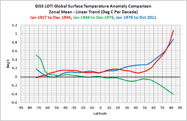
What my eyes see is moderate Arctic warming mostly over the Americas from 1880 to 1917, extreme zonal Arctic warming from 1917 to 1944, extreme Antarctic zonal Antarctic warming from 1944 to 1976 as average lower tropospheric temperatures supposedly cooled, and extreme zonal Arctic warming ever since.
Forget the trend lines, this is the message. Does Antarctic warming =”global” cooling? If so, why? The reciprocal question applies to the Arctic.
To whatever extent the old saw, “lies, damned lies, and statistics” is true, it is true of trend lines. I could draw you a trend line from the Eocene that would show us headed for a snowball earth, which to the best of our knowledge has never happened.
Statistical signal does not lie in averages. Statistical signal lies in the structure.
A blog post here :
http://blog.hotwhopper.com/2013/04/tisdales-tricks.html?spref=tw
is saying you are using tricks in this article.
Note, I’m just the messenger.
Is it probable that we’re seeing the beginnings of a late 20th/early 21st century flat period?
The periods seem to be a “cycle” – from early cooling period (1880 to 1917) covering 37 years, the early warming period (1917 to 1944) covering 27 years, the mid-20th century flat temperature period (1944 to 1976) covering 32 years, and the late warming period (1976 to 2012) now going into its 36th year.
If, as some say, we’ve started another flat period (starting about 16 years ago), how does that fall into your chart? It looks like that would be the worst “divergence” from the models.
garymount: Thanks for the link.
i repeat past comments:-
If the models do not follow reality the models ARE WRONG. So change the theory that spawned the models not the real time data.
The theory of the GHE is WRONG. Non of its claims have been found. No hindcasting has been correct. No science shows that CO2 drives climate. What else do these alarmists need, the voice of God?