Guest Post by Willis Eschenbach
Well, after my brief digression to some other topics, I’ve finally been able to get back to the reason that I got the CERES albedo and radiation data in the first place. This was to look at the relationship between the top of atmosphere (TOA) radiation imbalance and the surface temperature. Recall that the IPCC says that a change in the TOA radiation of 3.7 W/m2 from a doubling of CO2 will lead to a 3°C ± 1.5°C temperature increase. This 3°C per doubling is called the “climate sensitivity”, and its value is an open question.
Figure 1, on the other hand, shows my results regarding the same question of the climate sensitivity. These reveal nothing like a 3°C temperature rise from a doubling of CO2:
 Figure 1. Gridcell-by-gridcell linear trends of the change in surface temperature (∆T) given the change in TOA radiation (∆F). Note that the surface temperature data is gridded on a 5°x5° gridcell, while the CERES TOA radiation data is on a 1°x1° gridcell basis. Graph includes a two-month lag between change in forcing and the change in temperature.
There are a variety of interesting aspects to this particular graph. Let me start by describing how I constructed it.
I began by taking the gridded HadCRUT3 temperature data for the period of the CERES study, Jan 2001 to Oct 2005. The HadCRUT data is on a 5°x5° gridcell, so I first expanded that to 1°x1° gridcells. Then I took the first differences (∆T) by subtracting each month from the succeeding month, to get the monthly change in temperature (∆T) in each gridcell.
Then I compared that ∆T dataset to the change in TOA radiation (∆F), which was constructed from the CERES TOA data. For each gridcell, I took the linear trend of the temperature changes ∆T with respect to ∆F.
Of course, the climate sensitivity results from this procedure are in units of temperature change per forcing change, which is °C per watt/square metre. To convert it to change in temperature per doubling of CO2, I multiplied the results by 3.7 W/m2 per doubling of CO2.
Finally, I needed to adjust for the lag in the system. I did this in two ways. First, I selected the lag which gave the largest temperature change, which was a two month lag. These are the results shown in Figure 1. However, this is a cyclical record of the annual fluctuations, so the equilibrium sensitivity will be underestimated. Per the insights gained from my last analysis, “Time Lags in the Climate System“, the time lag is related to the size of the reduction in temperature swing. A 1-2 month lag in the system indicates a reduction in fluctuation of about 50%. So for my final adjustment, I doubled the indicated climate sensitivity. The results of this are the values shown in Figure 1.
Now, I have long argued, solely from first principles, that climate sensitivity is a non-linear function of temperature. I have said that the sensitivity was greater when it is colder, and that it is smaller when it is warmer. I have held that this relationship was non-linear, with a kink at the temperature range for tropical thunderstorm formation. Finally, I have also argued that in some places in the tropics the climate sensitivity is actually negative, due to the action of tropical clouds and thunderstorms.
To test these claims, I plotted the sensitivity for each gridcell shown in Figure 1 against the annual average temperature for that same gridcell. The results are shown in Figure 2. As far as I know, this is the first observational evidence that shows the actual relationship between climate sensitivity and temperature, and it supports all of my contentions about that relationship.
 Figure 2. Scatterplot of gridcell climate sensitivity versus gridcell temperature. Colors indicate the latitude, with red at the tropics, yellow in the temperate zones, and blue at the poles. Gray dashed line shows the linear trend, indicating that the climate sensitivity varies generally as -0.009 * temperature + 0.32 (p-value < 1e-16).
There are some important things about this plot. First, it strongly supports my claim that the climate sensitivity varies inversely with the temperature. Next, it shows that a number of areas of the tropics actually do have negative climate sensitivity. Finally, it shows that the relationship is non-linear with a kink at around the temperature for the formation of tropical thunderstorms. This is important corroborative evidence for my hypothesis that the tropical clouds and thunderstorms act as governors of the tropical temperature and are the source of the negative climate sensitivity.
Let me close by railing a bit against the pernicious nature of averages. Consider Figure 2. Normally, far too many climate scientists would take an average of that data, and come up with some number as the average climate sensitivity. But that number is meaningless, and worse, it gives the impression that the sensitivity is a fixed number. It is nothing of the sort. Not only is it not fixed, it is far, far from linear, and it goes negative at times. It is a dynamic response to changing conditions, not some fixed value.
As a result, when we average it, we come away with entirely the wrong impression of what is happening in that most complex of phenomena, the climate system. While averaging is often useful, it conceals as much as it reveals, and it can lead one to badly erroneous conclusions. That is why so many of my graphs and charts show thousands of individual points, as in Figure 2. Only by seeing the whole picture can we hope to understand the system.
My best to all,
w.
Willis mentions being a revolutionary. May I make that claim too ?
You guys don’t know what revolution is, you never lived through one, but since we are talking about the climate’s causes and consequences
this is the revolution
http://www.vukcevic.talktalk.net/Aa-TSI.htm
http://www.vukcevic.talktalk.net/Arctic.htm
For the benefit of laymen like me, are there any physicists out there who could hazard an exegesis of Mr. Eschenbach’s following explanation for why he multiplied his sensitivity value by two: “the time lag is related to the size of the reduction in temperature swing”? to
to  and its temperature
  at time
  is uniform in the
  and
and  directions. Then, if
  is the heat per unit area the slab contains below
  (where
  increases in the downward direction), the heat flow can be expressed as:

 is the slab’s thermal conductivity,
  , and
, and  is some arbitrarily chosen nominal temperature.

 is slab’s mass density and
  is its heat capacity.

 is the slab’s thermal diffusivity.
 surface. In the case of the irradiated earth, that is, we are making the simplifying (and highly questionable) assumption that radiation penetration is negligible. And we’ll assume that the (by assumption, uniform) temperature at the surface varies sinusoidally, i.e.,
  , where
  is the amplitude of the sinusoidal temperature variation at the
  slab surface. Furthermore, we’ll assume Geiger’s relationship that with depth the amplitude decays exponentially and the phase lag increases linearly:

 is the reciprocal of skin depth,
  is the sinusoid’s radian frequency (i.e.,
  divided by the sinusoid’s period),
  is the rate of phase-lag increase,
  , and we assume that
  is the only unknown. We find
  ‘s value by plugging our solution into the heat-flow equation:
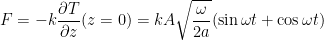
![\displaystyle -a\gamma^2 [A \exp i(\omega t + \gamma z)]=i\omega[A \exp i(\omega t + \gamma z)]](https://s0.wp.com/latex.php?latex=%5Cdisplaystyle+-a%5Cgamma%5E2+%5BA+%5Cexp+i%28%5Comega+t+%2B+%5Cgamma+z%29%5D%3Di%5Comega%5BA+%5Cexp+i%28%5Comega+t+%2B+%5Cgamma+z%29%5D&bg=ffffff&fg=000&s=0&c=20201002)
 :
:
 values into our equation for temperature
  yields:

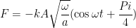
 into the slab (read “the net radiation absorbed by the earth’s surface”) is given by

 , i.e., by one-eighth of a cycle. Note that this is independent of what the frequency- and material-dependent attenuation is. Now, this is surface radiation, not top-of-the-atmoshphere radiation. But, if the top-of-the-atmosphere net radiation is essentially in phase with the surface net radiation, would that not suggest that the eighth-cycle lag observed by Mr. Eschenbach has little to do with the Geiger relationships he cites?
Please pardon the excruciating detail in which I set forth the problem that explanation gives me; I am hoping thereby to make manifest the misapprehension under which I seem to be laboring.
The flow of heat by conduction through a homogeneous material is proportional to the temperature gradient. For example, suppose a semi-infinite homogeneous slab extends from
where
Also, the temperature changes proportionally to the heat-flow gradient, i.e.,
where
Combining those two relationships gives:
where
Let’s consider the situation in which heat is introduced into the slab only at its
where
and solving for
Plugging one of the thus-determined
That was the wind-up. Here’s the pitch: The net heat transfer
That is, the net surface radiation leads the surface temperature by
I do not even know where to begin to address this piece by Mr. Eschenbach.
The Time lag for example. You talk about a time lag on a diurnal basis and on a monthly basis (seasonal) and even link us to another piece written by yourself about the lag. If there is a two month time lag in the seasonal system then surely there must be a time lag of decades in the climate system before it will start to warm up seriously.
What do you know about the time lag in the climate system or is it instantly warm when CO2 starts to rise in a “cold” world? Let’s make it more comprehensible: Is a living room of 15°C instanly warm when you crank up the heater to 20°C or does it take a while before the room reaches that temperature and what about the time needed when the room reaches equilibrium stage?
“I have said that the sensitivity was greater when it is colder, and that it is smaller when it is warmer.”
“This is important corroborative evidence for my hypothesis that the tropical clouds and thunderstorms act as governors of the tropical temperature and are the source of the negative climate sensitivity.”
– Can you also tell us what the tropical mean surface temperature is?
– Have you ever heard of the expanding of the tropical region to Northern and Southern lattitudes because these colder regions are more sensitive and thus warm up faster?
– Do you know that we had such conditions in the past where it was tropical on higher lattitudes?
Here is a piece from which you actually can learn something:
http://phys.org/news/2011-07-hot-earth-scientists-uncovers.html
It’s exactly what you are describing here and in complete agreement with a warming world due to increasing CO2.
Only your sensitivity numbers don’t fit and they are wrong. I asked you several questions about the same subject before in some of your previous blogs. You never answered them. If you want to conduct science here you should be courteous enough to answer these questions. That’s what science is all about.
You need to explain the basics of climate science first in order to reconcile the strong negative feedback by water vapor (hence tropical thunderstorms and clouds) in your hypothesis. I gave you a good explanation that your hypothesis of strong negative feedback is simply wrong.
You also need to explain why a doubling of CO2 (causing a 1-1.2°C rise when nothing else changes – every climate scientist agrees on this) causes less warming by the extra increased water vapor by that initially increased CO2. You need to explain how much extra water vapor is evaporated by doubled CO2 and why it causes such a strong negative feedback. All of this you need to back up with what has been written in the scientific literature about it. That’s science.
Also the Total and Observed Greenhouse Effect would not make sense anymore in your hypothesis when true. It’s basic physics.
You are conducting an experiment in a cold world getting ready to warm up by increasing CO2 due to the climate time lag. Surprisingly you are accepting the lag diurnally and seasonally, but you are leaving out this very important climate time lag of maybe hundreds of years.
You are nothing more than measuring the temperature in a room that is beginning to heat up before it reaches it’s destined temperature setting. And from these findings you are trying to produce some claims.
I can agree that thunderstorms and clouds will have a somewhat stronger negative feedback in tropical regions than elsewhere, but not in the milder and colder regions of the planet. Exactly the reason why the tropics don’t warm up that much in a warming world.
“this is the revolution”
Yes, vuk, we are all revolting. 🙂
Joe Born: “But, if the top-of-the-atmosphere net radiation is essentially in phase with the surface net radiation, would that not suggest that the eighth-cycle lag observed by Mr. Eschenbach has little to do with the Geiger relationships he cites?” phase that is independent of the sensitivity. And, since a lead of approximately that size between the top-of-the-atmosphere net radiation and the surface temperature is what Mr. Eschenbach’s data exhibit, that sensitivity-independent quantity appears to dominate the observed lead/lag, so I’m still struggling with how he obtains a sensitivity adjustment out of the observed phase lead.
I put that poorly. Personally, I would actually expect the top-of-the-atmosphere net radiation to lead the net radiation absorbed by the surface rather than be in phase with it. But my discussion above seems to indicate that this absorbed radiation will in turn lead the surface temperature by a fixed,
Stephen Wilde says:
June 20, 2012 at 3:00 am
Actually Philip I think that cloud amounts have a greater effect the nearer the equator the clouds are because the intensity of the reflected light is greater and that light energy is then no longer available to enter the oceans and contribute to the ENSO energy budget.
Stephen. you missed the point, which I stated rather tersely.
The significance of low level aerosols and seeded clouds is that they affect solar insolation predominantly when solar radiation traverses the atmosphere at a low angle. That is, in winter at mid-latitudes, in summer at high latitudes, and in the early morning everywhere.
Joe Born says:
June 19, 2012 at 9:10 pm
Joe, I noted in the last post that there is a relationship between the amount of the lag, and the attenuation of the signal. The relationship was such that with a 1-2 month lag in a system, the signal is attenuated to about half its original size.
Now, it’s obvious that any climate sensitivity that is calculated directly from annual variations in the temperature is attenuated by some amount from the actual signal. But how much will it underestimate it by? I needed to pick a number, and my best estimate for that value is the number I calculated from my previous post, that is to say, the attenuation indicated by the lag.
If you have a better estimate, that’s fine. But that’s the one I used. It’s not hugely significant, because it doesn’t affect my conclusions about a) the variability of the climate sensitivity with temperature, or b) the existence of large areas of negative climate sensitivity.
w.
Stephen Wilde says:
June 20, 2012 at 3:00 am
Cite for the poles cooling when the rest of the globe is warming and vice versa? I don’t find that anywhere in the data.
Thanks,
w.
Willis Eschenbach: “If you have a better estimate, that’s fine. But that’s the one I used. It’s not hugely significant, because it doesn’t affect my conclusions about a) the variability of the climate sensitivity with temperature, or b) the existence of large areas of negative climate sensitivity.”
As you may have inferred, no, I don’t have a better estimate. And my (not-very considered) opinion is in line with yours: the issue I raise not hugely significant, at least as to your main points. I’m merely trying, in my plodding way, to learn something from your (fascinating) previous post, but, for the reasons I gave in my last two comments, I haven’t been able to jump from those Geiger equations (which I essentially derive above) to the use you’ve put them to here.
I understand completely if you consider this issue a mere distraction. At the same time, I will be grateful if one of the more theory-minded physics types out there can set me straight.
Willis said:
“Cite for the poles cooling when the rest of the globe is warming and vice versa? I don’t find that anywhere in the data”
It seems to have applied during the Eemian warm period..
http://wattsupwiththat.com/2012/06/15/study-shows-the-arctic-was-much-colder-while-earth-was-warmer-during-eemian-warm-period/
During the late 20th century warming spell the Antarctic got colder but I would say that the Arctic doesn’t follow the pattern so closely because of warm water entering the Arctic Ocean from the south.
Furthermore the isolation of the polar air masses when the polar vortices are positive is well accepted and a warming world is supposed to accompany more positive AO and AAO.
see here:
http://en.wikipedia.org/wiki/Arctic_oscillation
“When the AO index is positive, surface pressure is low in the polar region. This helps the middle latitude jet stream to blow strongly and consistently from west to east, thus keeping cold Arctic air locked in the polar region.”
Possible explanation for why the increase in temperature is limited to the non-tropical NH. When CO2 enters the atmosphere, it does so by burning of hydrocarbons or respiration, both of which also add H2O. It’s the H2O, in the form of water vapor, that has the greater IR and warming effect. Since H2O precipitates out, over a period of days to weeks, an increase in NH H2O would have little effect on SH H2O. And in the tropics, an increase in H2O would lead to clouds and rain, increasing albedo and radiation loss to space via convection.
So I would expect that an increase in CO2 would raise temperatures primarily where there is a persistent increase in absolute humidity, and without a large increase in albedo/convection, and would not consider this a feedback, but rather a reflection that original CO2 increases and H2O increases are due to respiration and burning of hydrocarbons. One would need humidity observations at both the surface and at various altitudes to confirm, and I don’t know if our observations include enough humidity detail to test the hypothesis.
Stephen Wilde says:
June 20, 2012 at 11:05 am
Ah. My bad, Steven, I thought you were referring to the present time, which is why I asked.
w.
Robbie says:
June 20, 2012 at 7:41 am
In that case, you shouldn’t have begun.
Robbie, if you had been even mildly polite instead of snarkily condescending, I would have been glad to clarify your questions, point by point, as is my usual habit and general custom.
In your case, however, I’ll make an exception. You get nothing except the joy of knowing that your arrogance has prevented you from achieving your stated goal. Next time, keep a civil tongue in your head, you’ll find that people here will be more than happy to discuss science with you. As it is … not so much.
w.
You are talking like a Real climate scientist now, Willis. Don’t be petulant. It doesn’t help your credibility.
Robbie says: June 20, 2012 at 7:41 am
“…Here is a piece ….:
http://phys.org/news/2011-07-hot-earth-scientists-uncovers.html ….”
Thanks Robbie, interesting information: So the much warmer world of the early Eocene was much warmer at the poles and much the same as now in the tropics? (and an aside: doesn’t THAT sort of warmer world sounds like it might possibly be VERY productive?)
Seems to support Willis’ argument. The interesting thing is his observation that he is already seeing evidence of a lower sensitivity to ‘current forcings’ at lower latitudes.
.
Of course, the questions remain, what caused that temperature shift of the early Eocene, and was increasing carbon dioxide a cause or a result?
Joe Born says:
June 20, 2012 at 10:29 am
Joe, I have never seen a single one of your comments that is a “mere distraction”. And I was fascinated by your math above, I just haven’t had time to fully understand it. , is an independent constant. The part I don’t understand is this:
The question I would pose to you is this: I see where the surface heating is going to lag a cyclical radiation source. And although I haven’t had time to check your math, I see that the lag,
The part that is unclear is, since the earth is generally at thermal equilibrium, the net heat transfer into the slab over a full cycle ≈ zero … I don’t understand how that fits with your equation. Is that instantaneous heat transfer? If so, can it be integrated to give us the sensitivity? These questions and more …
Many thanks, and always good to hear from you. Oh, btw, you were 100% right and I was wrong in the previous thread about the trend of x on y NOT being the reciprocal of the trend of y on x, I just happened to pick a dataset where that was the case.
w.
Don Monfort says:
June 20, 2012 at 4:07 pm
Sorry, Don, but if someone wants to come in and talk down to me and be all snarky, I feel like I owe him an explanation as to why I’m ignoring him. Or would you advise I just ignore him and say nothing?
Because I won’t answer that kind of snide attack—I have far too many calls on my time, and people who are interesting and polite making fascinating comments, to respond to some jerkwagon who wants to insult me.
So how should I respond?
w.
markx-The Eocene is a very interesting case of past climate variability. The earliest analyses actually found cooler tropical temperatures than the present. Naturally this was “fixed” to make models look better, and now it is claimed that the Eocene had warmer tropics…but the diminishing of the Equator to Pole temperature difference is still greater than models appear to be able to explain.
If the tropical corrections are actually wrong…
Willis Eschenbach: “The part I don’t understand is this: ‘The net heat transfer into the slab (read “the net radiation absorbed by the earth’s surface”) is given by
 ‘
‘
 into the equation stating that heat transfer is proportional to temperature gradient, i.e., into
  .
.

The part that is unclear is, since the earth is generally at thermal equilibrium, the net heat transfer into the slab over a full cycle ≈ zero … I don’t understand how that fits with your equation. Is that instantaneous heat transfer?”
That expression is indeed (if I have this right) the instantaneous heat transfer, so it is consistent with the heat transfer’s being ≈ zero over a full cycle. I got it by plugging the solution
Willis Eschenbach: “If so, can it be integrated to give us the sensitivity?”
Well, I’ve been trying to infer sensitivity from it somehow, but I’m a little weak (okay, clueless) at differential equations (and my wife’s kept me busy shopping for patio furniture) so I’m pessimistic. But I’ll sleep on it.
By the way, at least one of the equations above has an error. It should be:
That is, the minus sign originally in the middle expression should have been a plus sign. [Fixed. w.]
“Ah. My bad, Steven, I thought you were referring to the present time, which is why I asked.”
The rest of my post did refer to the present time.
Joe, I’ve been playing with your equations. You say:


 gives us

I looked at the right hand side of that, which is:
Canceling out common terms and substituting
But when I try those two, I get different curves, viz:
Curiously, your old equation with the “-” in place of the “+” works out perfectly … so I’m in mystery here.
w.
PS—After much experimentation, I’ve found that using the LaTEX tag “\displaystyle” makes the latex much more readable.
whatever
Joe, I’ve found at least part of the problem, with the always invaluable aid of Mathematica:


Note that where you have
Mathematica, on the other hand, says:
Next, the right hand side of that in turn resolves to
or alternately to
(note the minus sign in front)
I haven’t checked the earlier part of your derivation yet.
w.
Don Monfort says:
June 20, 2012 at 11:19 pm
I gave you a reasoned reply to your objection above, and I asked you how you thought I should have responded Robbie … and that’s your answer?
Whatever … I should learn to never wrestle with pigs, I just get dirty, and the pigs like it.
w.
Willis Eschenbach: “Joe, I’ve found at least part of the problem.” , where
  is some fixed level of incoming radiation at the surface,
  is the unit step function, and
  is the radiation leaving the surface. I don’t suppose Mathematica could solve it? (I probably could have bought Mathematica for what I paid for patio furniture.)
Sorry about the “correction.” Somehow I can never keep track of canceling minus signs. If I differentiate it again I’ll probably get yet another combination of plus and minus signs.
So I’m unlikely to be equal to solving the one-dimensional wave equation for a semi-infinite slab with the initial condition T(z,0)=0 and the boundary condition