Radiative Physics Simplified II
A guest post by Jeff Id
Radiative physics of CO2 is a contentious issue at WUWT’s crowd but to someone like myself, this is not where the argument against AGW exists. I’m going to take a crack at making the issue so simple, that I can actually convince someone in blogland. This post is in reply to Tom Vonk’s recent post at WUWT which concluded that the radiative warming effect of CO2, doesn’t exist. We already know that I won’t succeed with everyone but when skeptics of extremist warming get this wrong, it undermines the credibility of their otherwise good arguments.
My statement is – CO2 does create a warming effect in the lower atmosphere.
Before that makes you scream at the monitor, I’ve not said anything about the magnitude or danger or even measurability of the effect. I only assert that the effect is real, is provable, it’s basic physics and it does exist.
From Tom Vonk’s recent post, we have this image:
 Figure 1
Short wavelength light energy from the sun comes in, is absorbed, and is re-emitted at far longer wavelengths. Basic physics as determined by Planck, a very long time ago. No argument here right!
Figure 2 below has several absorption curves. On the vertical axis, 100 is high absorption. The gas curves are verified from dozens of other links and the Planck curves are verified by my calcs here. There shouldn’t be any disagreement here either – I hope.
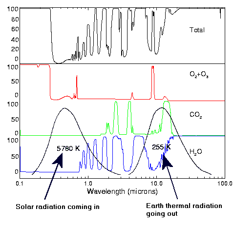 Figure 2 – Absorption curves of various molecules in the atmosphere and Planck curve overlay.
What is nice about this plot though is that the unknown author has overlaid the Planck spectrums of both incoming and outgoing radiation on top of the absorption curves. You can see by looking at the graph (or the sun) that most of the incoming curve passes through the atmosphere with little impediment. The outgoing curve however is blocked – mostly by moisture in the air – with a little tiny sliver of CO2 (green curve) effective at absorption at about 15 micrometers wavelength (the black arrow tip on the right side is at about 15um wavelength). From this figure we can see that CO2 has almost no absorption for incoming radiation (left curve), yet absorbs some outgoing radiation (right curve). No disagreement with that either – I hope. Tom Vonk’s recent post agrees with what I’ve written here.
Energy in from the Sun equals energy out from the Earth’s perspective — at least over extended time periods and without considering the relatively small amount of energy projecting from the earth’s core. If you add CO2 to our air, this simple fact of equilibrium over extended time periods does not change.
So what causes the atmospheric warming?
Air temperature is a measure of the energy stored as kinetic velocity in the atoms and molecules of the atmosphere. It’s the movement of the air! Nothing fancy, just a lot of little tiny electrically charged balls bouncing off each other and against the various forces which hold them together.
Air temperature is an expression of the kinetic energy stored in the air. Wiki has a couple of good videos at this link.
“Warming” is an increase in that kinetic energy.
So, to prove that CO2 causes warming for those who are unconvinced so far, I attempted a thought experiment yesterday morning on Tom Vonk’s thread. Unfortunately, it didn’t gain much attention. DeWitt Payne came up with a better example anyway which he left at tAV in the comments. I’ve modified it for this post.
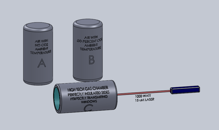 Figure 3- Experimental setup. A – gas can of air with all CO2 removed at ambient temp and standard pressure. B – gas can of air diluted by 50 percent CO2, also at ambient temp and standard pressure. C ultra insulated laser chamber with perfectly transparent end window and a tiny input window on the back to allow light in from the laser. Heat exit’s the single large window and cannot exit the sides of the chamber.
Figure 4 is a depiction of what happens when C contains a vacuum.
 Figure 4 – Laser passes straight through the chamber unimpeded and a full 1000 Watt beam exits our perfect window.
The example in Figure 5 is filling tank C with air from tank A air (zero CO2) at the equilibrium state.
 Figure 5 – Equilibrium of hypothetical system filled with zero CO2 air from canister A.
Minor absorption of the main beam causes infrared absorption and re-emission from the gas reducing the main beam from the laser. This small amount of energy is re-emitted from the gas through the end window and scattered over a full 180 degree hemisphere.
What happens when we instantly replace the no-CO2 air in chamber C with the 50% CO2 air mixture in B?
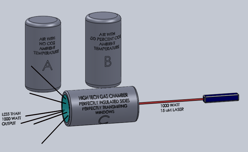 Figure 6 – Air in C is replaced instantly with gas from reservoir B
From the perspective of 15 micrometer wavelength infrared laser, the CO2 filled air is black stuff. The laser cannot penetrate it. At the moment the gas is switched, the laser beam stops penetrating and the 1000 watts (or energy per time) is added to the gas. At the moment of the switch, the gas still emits the same random energy as is shown in Figure 5 based on its ambient temperature, but the gas is now absorbing 1000 watts of laser light.
Since the beam cannot pass through, the CO2 gains vibrational energy which is then turned into translational energy and is passed back and forth between the other air molecules building greater and greater translational and vibrational velocities. —- It heats up.
As it heats, emissions from the window increase in energy according to Planck’s blackbody equation. Eventually the system reaches a new equilibrium temperature where the output from our window is exactly equal to the input from our laser – 1000 watts. Equilibrium! – (Figure 7)
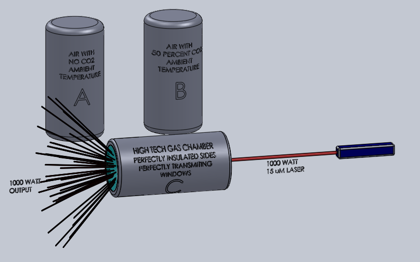 Figure 7 – Equilibrium reached when gas inside chamber C heats up to a temperature sufficient to balance incoming light energy..
The delay time between the instant the air in C is switched from A type air to B air to the time when C warms to equilibrium temperature is sometimes stated as a trapping of energy in the atmosphere.
“CO2 traps part of the infrared radiation between ground and the upper part of the atmosphere”
So from a few simple concepts, two gasses at the same temp, one transparent the other black (at infrared wavelengths), we’ve demonstrated that different absorption gasses heat differently when exposed to an energy source.
How does that apply to AGW?
The difference between this result and Tom Vonk’s recent post, is that he confuses equilibrium with zero energy flow. In his examples and equations, he has a net energy flow through the system of zero, which is fine. Where he goes wrong is equating that assumption to AGW.
What we have on Earth, is a source of 15micrometer radiation (the ground) projecting energy upward through the atmosphere, exiting through a perfect window (space) – sound familiar? Incoming solar energy passes through the atmosphere so we can ignore it when considering the most basic concepts of CO2 based warming (this post), but it is also an energy flow. In our planet, the upwelling light at IR wavelengths is a unidirectional net IR energy flow (figure 2 – outgoing radiation), like the laser in the example here.
Of course adding CO2 to our atmosphere causes some of the outgoing energy to be absorbed rather than transmitted uninterrupted to space (as shown in the example), this absorption is converted into vibrational and translational modes (heating). Yes, Tom is right, these conversions go in both directions. The energy moves in and out of CO2 and other molecules, but as shown in cavity C above, the gas takes finite measurable time to warm up and reach equilibrium with space (the window), creating a warming effect in the atmosphere.
None of the statements in this post violate any of Tom’s equations; the difference between this post and his, is only in the assumption of energy flow from the Sun to Earth and from Earth back to space. His post confused equilibrium with zero flow and his conclusions were based on the assumed zero energy flow. The math and physics were fine, but his conclusion that insulating an energy flow doesn’t cause warming is non-physical and absolutely incorrect.
Oddly enough, if you’ve ever seen an infrared CO2 laser cut steel, you have seen the same effect on an extreme scale.
————-
So finally, as a formal skeptic of AGW extremism, NONE of this should create any alarm. Sure CO2 can cause warming (a little) but warmer air holds more moisture, which changes clouds, which will cause feedbacks to the temperature. If the feedback is low or negative (as Roy Spencer recently demonstrated), none of the IPCC predictions come true, and none of the certainly exaggerated damage occurs. The CO2 then, can be considered nothing but plant food, and we can keep our tax money and take our good sweet time building the currently non-existent cleaner energy sources the enviro’s will demand anyway. If feedback is high and positive as the models predict, then the temperature measurements have some catching up to do.
Even a slight change in the amount of measured warming would send the IPCC back to the drawing board, which is what makes true and high quality results from Anthony’s surfacestations project so critically important.
This is where the AGW discussion is unsettled.
====================================
My thanks to Jeff for offering this guest post – Anthony
Jim D, August 10, 2010 at 5:24 pm
(1) At 100mb, peaks in P- and R-branches are 300 times higher than their average. Check with spectralcalc.com. It is pretty much clear that “average emission height” is not where it is believed to be, and change in it does not have the warming effect.
(2) This is technically not an error with resolution. The error is in more subtle mathematics of averaging order.
(3) There is no surprise that static under-resolved calculations match the shape of under-resolved observations. However, the _change_ in absolute value of emission integral is completely different thing. Convincing observations of this change are lacking.
Al Tekhasski :August 10, 2010 at 8:05 pm
Thanks for the spectralcalc.com link. Neat tool, even just the free access part.
Obviously the combination of their strength and sparseness has to be represented somehow at lower resolution. I can’t claim to know much about how MODTRAN does that, but I imagine someone has done the same integrated calculations with HITRAN and compared them, and I would like to know how that turned out, and am unconvinced there could be much difference relative to the CO2 doubling signal.
Al Tekhasski says:
August 10, 2010 at 8:05 pm
Jim D, August 10, 2010 at 5:24 pm
(1) At 100mb, peaks in P- and R-branches are 300 times higher than their average. Check with spectralcalc.com. It is pretty much clear that “average emission height” is not where it is believed to be, and change in it does not have the warming effect.
———-
I’ve got a radiative transfer model with variable resolution using HITRAN. Currently, I’m running about 10nm wavelength bin widths. Initially, I used 1 nm widths. Some lines fit inside 1nm but most do not. I usually run it from 0.1 to 75 um. Actually, over very limited bandwidths, a few Angstroms, I’ve run it down to 0.005 Angstrom resolution also – amazing how you can see the equipment smearing present on some of the highest resolution stellar spectrums ever done in comparison.
The net result though is that 1nm merely made it time consuming to process the data. While there was still a few W/m^2 of power at wavelengths longer than 75um (difference between the sum of the bins and stefan’s law), there was somewhat less difference between the 10nm and 1nm resolution. My model also broke down the atmosphere into over 50 layers with the bottom being 1km slabs, each with their own temperature, pressure, and composition.
effects of each layer are substantially different in the troposphere. Lower, one has much broader lines and it’s easy to see just looking at the patterns in the array of raw numbers in the excel spread sheets.
Results for a co2 doubling comes out to about 3.6 W/m^2 at the tropopause and about 2.6 at the 120km altitude. This is clear sky only and radiative only and excludes feedbacks. The 120km altitude is likely inaccurate as LTE is a problematic assumption above the stratosphere, although it appears valid for co2. By assuming a uniform rise in T for the entire column along with constant relative humidity, one can also get an idea of what the ‘primary’ feedback (more h2o vapor) is going to do. An assumption of 5 deg C would result in the absolute humidity increase of 30% – which is a long way from a doubling of h2o vapor. An increase of of 2 deg C results in only a 13% increase. Despite h2o having a stronger effect per doubling than co2, one finds that the 5 deg C rise with a co2 doubling results in a total increase in radiative absorption of under 6 W/m^2, which is less than twice what the co2 only effect would be. A 2 deg C rise would result in an increase to less than 5W/m^2.
If one goes back to simple averages to get an idea of sensitivity, one finds that a 288k temperature body of emissivity = 1 would emit 391 w/m^2 and that planet Earth receives 341 w/m^2 solar incoming power – of which 0.3 is reflected away, leaving 239 w/m^2 to be absorbed. For balance that means only 239 w/m^2 can be emitted away. For clear sky, that means 391-239 = ~150 w/m^2 average absorption of outgoing surface power (including cloudy conditions). With a 33 deg C rise from the theoretical BB object radiating 239 w/m^2, one can get the average sensitivity as 33/150 = 0.22 K rise per W/m^2 increase.
Applying this sensitivity, one has a contribution for a co2 doubling, including the ‘primary’ feedback of h2o vapor that amounts to just over 1 deg C (0.22 x ~5w/m^2). And that leaves us missing almost another degree’s worth of power absorption still needed to achieve that amount of T rise.
Not that the clouds are quite complex in contributions. We’ve got about 62% cloud cover of all types, each with their own effects. During the day, they contribute substantially to the albedo, sky = 0.22 while surface = 0.08 of the 0.30 total. At all times, they absorb most of the outgoing IR and reradiate a full continuum from their tops (at their characteristic temperature – which is much cooler than the surface). The net result is to provide a slight cooling effect – but not as much as one would assume. That is, the more clouds, the cooler – but not by a bunch.
In clear skies, there’s about 280 w/m^2 escaping (much more than permissible for balance with current albedo, but there would also be a loss of 0.22 worth of albedo which means the balance point would shift to 313 w/m^2 – requiring an increase of T. Note that 280 w/m^2 in clear skies means that there’s 391-280 = ~110 w/m^2 of actual GHG absorption and for the surface emission, only 280/391 = 0.7 fraction of surface emissions escape. For this ‘world’ with no clouds, balance would require (313-280 )/ 0.7 = 47 w/m^2 additional surface emissions. Using stefan’s law, with 391 + 47 w/m^2, we get a final T of 296.5k which is a rise of 8.3 deg C due to a complete loss of cloud cover.
Note that the spectrum of radiated power is quite complex. Absorption from h2o vapor and co2 isn’t total because it will radiate outbound at some altitude (and temperature). No two wavelengths will have exactly the same altitude as the path length varies even depending upon where on an individual spectral line one is looking.
If you want a laugh, go read Hansen’s paper published in some national geographic publication around 1998. In it, he establishes an altitude using stefan’s law and the whole power emission of an assumed black body and then tries to show what the emission temperature change with lapse rate will be from the change in that altitude and how it must heat up to permit the level of original emission again.
cba, that was a very comprehensive report, thanks.
However, you are considering too many things at once. We have here an entirely theoretical discussion about effect of “instant” doubling of CO2 without any feedbacks or else. So please let’s start from basic conditions:
(a) we are considering, say, Standard USA temperature profile, with fixed lapse rate across troposphere, and fixed temperature gradient in stratosphere;
(b) we are looking at total OLR in the energy-containing range from 50 to 2500 cm-1, or just between 600 and 800 cm-1, where the IR windows end and CO2 absorption peaks.
(c) the question is: what is the _change_ in outgoing radiance in this range if CO2 concentration is instantly doubled, say from 400 to 800ppm.
Now few technical questions for you:
1. Is this true that you can do this in Excel?
2. What do you mean “50 layers”? What are the assumed conditions between slabs?
3. How do you account for variable temperature-pressure broadening? Which waveform shape do you assume?
4. For strongly opaque lines, how do you account for scattering?
More questions to follow…
Al Tekhasski says:
August 11, 2010 at 12:00 pm
(a) we are considering, say, Standard USA temperature profile, with fixed lapse rate across troposphere, and fixed temperature gradient in stratosphere;
(b) we are looking at total OLR in the energy-containing range from 50 to 2500 cm-1, or just between 600 and 800 cm-1, where the IR windows end and CO2 absorption peaks.
(c) the question is: what is the _change_ in outgoing radiance in this range if CO2 concentration is instantly doubled, say from 400 to 800ppm.
Now few technical questions for you:
1. Is this true that you can do this in Excel?
2. What do you mean “50 layers”? What are the assumed conditions between slabs?
3. How do you account for variable temperature-pressure broadening? Which waveform shape do you assume?
4. For strongly opaque lines, how do you account for scattering?
I use and think only in terms of wavelength rather than the per cm frequency of the spectrometry people. 25/cm is way down in the realm of radio mm microwave. Most of the spectral broadband emission occurs at 75 um and below. For dealing with situations of visible light, I go down to the relatively hard uV which is well beyond the IR cut off.of global T emissions.
Although not limited to it, I almost always use the 1976 std US atmosphere as it’s a well known, common, and rather typical or close to what one would consider as an average atmosphere. From there, I modify co2 and or h2o concentrations.
As such, an instant doubling (usually 330 to 660ppm as 330ppm is the 1976 value) results in a change of in radiation of a 3.6x w/m^2 decrease over the range of essentially 0 to 75um with a surface emission of 386 w/m^2 (288.2k emissions over 0-75um). And this value is at the tropopause of 11km. Drop another w/m^2 for 120km and take your risk of non LTE effects possibly occurring higher up.
I use excel for a portion but not all. I wrote a program to read the HITRAN processed output database from their javahawks application which creates a 296K 1 atm pressure database of lines. My program takes the line data, corrects it to the desired temperature and pressure and builds the contribution to the spectrum by wavelength bin for each line enabled. Most lines take up multiple bins but in all cases, the contribution to the entire bin is calculated. Calculations and adjustments are made according to the HITRAN documentation, Rothman 1996, appendix A found on the official HITRAN site. Input to my program includes a list of molecules to select and a number of layers to create along with the pressure and temperature for each layer.
Once my program has run, it creates an output file containing the transmission factor by wavelength per cm length for each layer. That is imported into a spreadsheet where additional processing is performed. This includes the BB spectrum and thicknesses for each layer. It is the excel program that determines the actual radiative transfer calculations are done by wavelength bin. Options include summing (integration) over wavelengths and graphing by wavelength.
The radiative transfer consists of the attenuation by wavelength within a layer and emissions generated by the gases in that layer. Lower levels are 1km thick while intermediate levels are 2.5km thick and high altitudes are 5km thick.
A temperature and pressure are assigned to each layer. I don’t recall if these are the bottom of the layer conditions or somewhere a portion of the way through the layer. It is an approximation but each layer has just one temperature assigned and one pressure.
there are no assumptions concerning between slabs. Each slab has assigned values and thicknesses and the radiation must go through each to reach a higher altitude or escape the Earth. Most 1-d models use about half that many or less from what I understand.
I use the line broadening approach provided in the Rothman 1994 paper appendix. Seems like it is a Gaussian curve that includes a peak shift due to pressure as well as width calculations based upon T and P. This allows for a reasonably precise calculation on the fly for each line to determine the amount of line contribution to the absorption of each bin that can execute in fast calculations.
Scattering is not handled in the program at present. We’re mostly dealing with fairly far IR here and it is 1/wavelength^4 as I seem to recall making it quite small. There’s way too many other parameters associated with the real world conditions that are just variable or unknown that have far greater effects upon the system than does a co2 doubling. There is also nothing on dimers involved or for that matter, aerosols in general. If you really try to deal with all these sorts of things, the requirements of what is required to in the way of starting data and conditions exceeds what could be known about the system. As you said above, it’s easy to try to consider too many things at once.
cba,
I agree with Al that the question, at this stage, is simply what happens to the integrated outgoing longwave in CO2 doubling for a standard atmosphere, looking down from about 70 km. I don’t have the software to do this, but testing the sensitivity to resolution would be interesting, and the band of interest is 600-800 /cm.
Your result of only 2.6 W/m2 at 120 km is a little surprising, which is why I would like to see if that varies with spectral resolution. This amounts to a CO2 forcing at the top of the atmosphere of about 0.7 K, instead of nearer 0.9 as others say, but maybe this is something that would vary according to the mean sounding chosen.
Just for reference; it appears that the savi.weber.edu HITRAN plotting tool has recently gone offline.
cba,
Could you please calculate just two numbers? After doubling in CO2, what is the change in OLR in two narrow bands, (a) 679.7-679.8, and (b) 680.7-680.8 cm-1, in your model? All looking down from 120km? Thanks.
jim d
I don’t recall there being a substantial difference with a change in resolution. Now with 1 nm resolution, I can only do 65um bandwidth and it is extremely difficult as a recalc in excel can take almost an hour on a larger and much faster computer as I am using now. I went to 10nm simply to cut down on the difficulties. Going to a much narrower bandwidth will have a substantial effect as there are contributions in addition to just the 15um band.
The lower power blocking at higher altitudes is due to the fact that even though the pressure is dropping, the temperature can be significantly hotter than the surface.
Note that the 10nm model gives 2.66 w/m^2 at 70km difference between 330 ppm and 660ppm of co2. Note that the modtran calculator is good out to about 70km and you can adjust the co2 values looking down and selecting the 1976 std atm US.
note that I ran the modtran calculator at http://geoflop.uchicago.edu/forecast/docs/Projects/modtran.orig.html for the 1976 atmosphere option, 70km and a doubling from 330 to 660ppm and wound up with 2.86 w/m^2 absorption – about 0.2 w/m^2 difference from my calculation. Note though that they go out to 100um compared to my 75um maximum wavelength and that they are using a totally different system from HITRAN.
Note that 70km is about the upper limit for the modtran calculator. above that I don’t think they actually do calculations beyond that despite an absence of warnings.
for whatever reasons, the 11km tropopause measurement differs a bit more in the wrong direction. The modtran calculator provides 3.4 w/m^2 while my calculations gives 3.7w/m^2 with the same differences in bandwidth mentioned above. I do not claim that my model is more accurate than the modtran calculator but it does provide a value in the ballpark of what the modtran calculator produces and also what the general climatology claim is and it is a bit closer to this claimed value than the modtran calculator produces for this situation.
Merrick
….”Many are going to immediately respond back regarding LTEs and forcings and negative feedbacks. Yes – of course they are all very important points to take into consideration. But this small portion of the topic seems still to be poorly understood by most of the folks here and it sure would be nice if we could get a significant plurality up to speed on at least this part.
A boy can dream, can’t he!”……….
I have found your posts on this topic rational and interesting.
However in the nature of things they must be partial to “stay on topic”
Any chance of Anthony inviting you to do a post giving the big picture on this topic?
Al Tekhasski says:
August 11, 2010 at 7:48 pm
cba,
Could you please calculate just two numbers? After doubling in CO2, what is the change in OLR in two narrow bands, (a) 679.7-679.8, and (b) 680.7-680.8 cm-1, in your model? All looking down from 120km? Thanks.
———
These are 14.710 – 14712 um and 14.689 to 14.691 um amount to 1/5 of the resolution I’m using. I made a special run for you for these at high resolution, 0.01 nm bin size. It was a bit more time consuming than expected.
at 2x co2, the power transmitted from 120km outward is:
14.689.00 to 14.691.00 um 0.018268837 W/m^2
14.710.00 to 14.712 um 0.018976876 W/m^2
at 1x co2:
14.689.00 to 14.691.00 um 0.017229193 W/m^2
14.710.00 to 14.712 um 0.019007363 W/m^2
tropopause
1x co2
14.689 to 14..691 um 0.0138603 W/m^2
14.710 to 14712 um 0.019035344 W/m^2
2x co2
14.689 to 14.691 um 0.0138603 W/m^2
14.710 to 14.712 um 0.019007948 W/m^2
I’m not sure what you hope to ascertain by these but they do seem to behave a bit differently from each other.
Al,
I don’t think you are going to get those two lines to contribute anything significant compared to the dense 667/cm spike. They are too widely spaced.
cba, it looks like your program calculates things in right direction.
In my example, the narrow 0.1cm-1 range (b) contains a medium-absorbing peak, one from the “R-branch” area of CO2 spectrum. The range (a) is between peaks, with weak absorption. This entire area is a part of CO2 15-um absorbing band, it has this typical fine structure everywhere.
From your results, the “weak” band (14.7113um) produces reduction in OLR by 0.00003W/m2, which is “consistent” with NEGATIVE imbalance, as per AGW theory.
Now, peak spacing in this area is 1.4cm-1. Therefore there are approximately 13 “weak” areas for each “strong” area. When averaged, the entire area will show NEGATIVE imbalance approximately 14*-0.00003= -0.0004W/m2. You can try to reproduce this number directly using 2cm-1 spectral resolution.
However, from your other result, the “strong band” (14.69um) produces an INCREASE in OLR, +0.001W/m2. The actual averaged OLR (1.4cm-1 band) is therefore +0.001-0.0004 = +0.0006 W/m2. The result is POSITIVE imbalance.
So, your result is a solid illustration that high-resolution spectrum produces OPPOSITE result to medium-resolution spectrum, at least in most important IR absorbing areas. Just as I said earlier, the overall official imbalance of -3.7W/m2 for CO2 doubling seems to be wrong, or highly inflated. Thanks.
Al Tekhasski,
I don’t agree with you on that conclusion on the basis of the fundamental physics. While at 120km, we should still be in LTE for co2, we’re probably not in LTE for NO and some other molecules. The atmosphere is above is quite thin (rather quite a good vacuum) and the temperatures are quite above mean surface T. That places the optical path at fairly large lengths and the likelihood of photon escape to be fairly good, especially in the wings where lower pressure reduces the likelihood of absorption and emission compared to lower levels.
These details are smeared into whatever resolution I’m dealing with, whether it’s 10 nm or 0.01 nm. Ultimately, the effect of the whole spectral line is considered, regardless of how many bins it fills and as the pressures decrease and the line narrows towards a zero bandwidth width line, it fits into one bin as a fraction of the bin. But then, we’re integrating the result over all the bins anyway.
While one might argue that an integration over dx provides a more accurate result than does a summation over delta x bins, that’s true only if the delta x bin values are averages that are approximate rather than integrated or if we’re dealing with a range that is not an integral multiple of the bin size. I take the integrated result of the line’s area under the curve in a non numerical methods approach.
If there were approximations involved (as in my first attempt), the results would be highly resolution dependent and without sufficient resolution, the results would be in error. However, I integrated the line function and attributed the appropriate amount of integrated result to each bin for each line of each molecule and these are using 39 molecules plus isotopes. The approach is no different for any resolution.
Since it’s using radiative transfer, each layer has an emission as well as absorption and the net is going to depend upon the Temperature spectrum incoming and on the temperature of the layer. The likelihood of emission is the same as the likelihood of absorption times the energy distribution (which is easiest to envision as the the planck BB spectrum curve for the temperature of the layer). Multiply one by the other at each wavelength and the emission curve is determined. That has the effect of showing that a gas cloud in front of a radiating surface will have emission lines if the gas cloud is hotter and absorption lines if it is cooler than the radiating surface and will have no lines if it is the same temperature.
cba, which “fundamental physics” you are talking about? I don’t think LTE has nothing to do with anything, you can try 70km. I think the result will be even better (for me). Also, we seems to have established that other molecules are out of the picture, so please forget them.
What was demonstrated here is that (a) the order of integration is critically important, and (b) spectral resolution has to be better than 1nm, otherwise the result is wrong.
When you integrate a line over your bin, you smear it, it’s effective emission height is much, much lower. It makes the whole difference when atmosphere has different temperature gradients with height. It was clearly demonstrated with your own numbers, the entire effect from CO2 doubling gets REVERSED, at least in this 14-16um zone.
So, what is left? The side edges of the band. However, these areas are literally “gray areas” of radiation physics, they fall right between “thin” and “thick” approximations. Would you agree that areas without good physical approximation could be prone to substantial computational uncertainty, softly speaking?
Al,
power is power per bandwidth. just because a particular bandwidth of 2nm shows increased emission while a nearby 2nm bandwidth shows increased absorption doesn’t mean that my program isn’t taking both into account in fewer bins when at 10nm bin resolution. The difference between 11km (tropopause) and 120km for total co2 absorption from a doubling is proof of that. At 11km, it’s 3.7w/m^2 over the 75um range. At 120km, it’s 2.6w/m^2. Clearly there was an increase in emissions higher up that made up for part of the difference from lower down.
As mentioned before, I actually integrated the width function before applying it in the software. Rather than smearing it, I have the area under the curve. Each line has a function of absorption vs wavelength and essentially, at low pressures, it’s very narrow and tall and at higher pressures it’s broader. To find out just how much that line blocks out of the continuum spectrum, one must integrate this function over the spectrum – that is over all of the spectrum that is affected by that line. One then has the total absorption involved. An integration over an entire range can be broken down into two integrations over two halves of that range or 4 integrations over the four quarters of the the range. Hence, when I sum the bins, I am combining the integrations already done into a final integration over the whole range of interest. BTW, these are done at each of the 50+ layers using an average P and T for that layer.
well, my model isn’t capable of being subtracted out from the high resolution measured spectral lines and show a perfect subtraction that allows simple computer processing of the result to eliminate atmospheric lines from the result. Actually, it almost can and can readily permit one to identify what lines originate in our atmosphere versus what lines are a genuine part of the incoming spectrum. And some of the problem can be attributed to the limiting resolution of the measurement apparatus and some can be attributed to the difference in a model typical atmosphere and in what the atmosphere was actually like during the measurements.
To make matters more interesting in this application, we are not dealing with two lines but thousands or tens of thousands of lines total. Inaccuracies of a few % which are random are going to be diminished to very small values by an averaging effect leaving only some sort of systematic error remaining.
there’s plenty of room for tremendous error overall. I doubt there’s much error in this for several reasons. First, the database has been developed over 30 + years for practical applications, more than a few are probably classified still. Second, when I can take a super high resolution slice of spectrum and compare with the calculations of the model and have to do averaging to smear it down to the resolution of the instrumentation and have the two appear visually identical, I’m pretty sure that you’re talking mole hills and not mountains. BTW, it wasn’t a solar spectrum and it is one of only three ever done at that high a resolution.
Where the inaccuracies lie are primarily in the fact that these are clear sky calculations. Over half the world is covered in clouds of one description or another at any one time. That totally scrambles the results right there. Cloud cover, cloud albedo, and total albedo toss in massive uncertainty. Clouds themselves do that by themselves on both the albedo front and on the IR blocking front.
cba, you wrote:
“power is power per bandwidth. just because a particular bandwidth of 2nm shows increased emission while a nearby 2nm bandwidth shows increased absorption doesn’t mean that my program isn’t taking both into account in fewer bins when at 10nm bin resolution.”
My example of integration (based on your excellent data) shows that your program calculates integrals wrongly. I suggested one narrow bit (0.1cm-1) at a peak absorption, and another in between peaks, with weak absorption. The overall spectrum structure is periodic, 1 strong bin, 13 weak bins, all based on HITRAN database and spectralcalc plotting routine. Then I integrated your emission results per a band of 14 bins, 13 at low absorption, and 1 at high. The result was POSITIVE change in OLR, while if I spread all stuff over 14 bins evenly, the result will be NEGATIVE, the one you are assuming as being correct. Since the spectrum structure is not random but nearly periodical, it is obvious that the result applies to thousands of nearly identical bins across the entire 14-16um band, and likely across all other spectral regions. This result of CORRECT integration is based on the same spectral data, 30 years of 150 years, I don’t care.
What I do care is that the order of averaging in all (yours included) OLR calculations does make profound effect on the global OLR integral. Averaging spectrum into bins that are wider than typical absorption peaks of CO2 before calculating path emission is mathematically incorrect procedure. Under atmospheric pressures of interest, 100-200ppm, these peaks have typical width of 0.1cm-1 (less than 1nm). Therefore, all results that use wider that 1nm spectral resolution in LBL calculations must be incorrect. Your data and my analysis prove this.
Re: “… have to do averaging to smear it down to the resolution of the instrumentation and have the two appear visually identical, I’m pretty sure that you’re talking mole hills and not mountains.”
Our joint result is based on detailed accurate physics: strong bin emits from stratosphere, and weak bins are transparent to IR and do not change much. The idea of smearing the spectrum down to instrumental resolution is a highly unwise one: the fact that instruments see the world through “murky lens” does not mean that the underlying physics becomes different. And the physics (as confirmed by your calculations) says that OLR increases with increase in CO2.
Regarding clouds: no, clouds do not scramble any of the above results, because spectrum lines behave independently. If a particular spectrum band of CO2 is masked under background emission “noise”, change in CO2 will not affect OLR anyway. If certain absorption lines outstand into stratosphere, the effect of CO2 increase results in higher OLR, or global cooling. Again, we are considering a hypothetical situation when all other things are equal. Therefore, masking and scrambling of areas between strong CO2 absorption peaks only enhances my result.
The inescapable conclusion is: the 3.7W/m2 radiative forcing from CO2 doubling is likely a very overstated number. For the same reasons the same conclusion is likely for all IPCC forcings from all other GH gases.
cba: “The difference between 11km (tropopause) and 120km for total co2 absorption from a doubling is proof of that. At 11km, it’s 3.7w/m^2 over the 75um range. At 120km, it’s 2.6w/m^2. Clearly there was an increase in emissions higher up that made up for part of the difference from lower down.”
This means that the optical path area above tropopause is quite important, and the direction of change is consistent with my concept of importance of stratospheric cooling for global radiative forcing. It also means that you program works correctly, even for the set of input parameters with very coarse resolution. Now if you re-calculate everything with 1nm resolution, I expect the difference will be much bigger, up to a reversal of entire result.
Al,
just to make sure you understood what I provided you, here it is again. The data I provided came from a narrow band run of 0.01 nm bin widths and the results were summed to provide 2nm width bands. The gas mix was the full 39 HITRAN data base molecules.
I do have some 1nm runs on another computer. I’ll have to try to dig them up. Also, they only go to 65um. I didn’t think there was any difference in the total power absrption.
as for my real project, it’s not about IR or outgoing emissions. It’s about atmospheric effects on incoming and it’s about identifying lines as being atmospheric or not.
Al,
I checked the other computer where I have 1nm resolution.
Both are adapted to 0.2 to 65.5um
the rest of the conditions are the same as mentioned previously
Here’s the following results:
1nm
11km 70km 120km
3.47 3.39 3.39 W/m^2
10nm
3.69 2.63 2.71 W/m^2
I don’t have the details as to whether the 1nm has the integration upgrades as it’s old and obsolete. However, you’ll note that the differences indicate it is still in the ball park.
“Yes, Tom is right, these conversions go in both directions. The energy moves in and out of CO2 and other molecules, but as shown in cavity C above, the gas takes finite measurable time to warm up and reach equilibrium with space (the window), creating a warming effect in the atmosphere.”
In the thought experiment, isn’t the CO2-heavy gas introduced into the cavity at ambient temperature and already in temperature equilibrium with the window? If so, in the time lapse referred to the gas doesn’t heat up, rather it is induced by the two-way excitation process, on which you agree with Tom, to emit at a rate to balance the laser input, though in a broader spectrum and in a diffused pattern?