Climate change debate – latest results

Guest essay by Bevan Dockery

Here is 38 years of empirical data clearly showing a relationship between the satellite temperature and the rate of change of atmospheric CO2 concentration at the Mauna Loa Observatory.

image

Figure 1. Mauna Loa Observatory

Figure 1 shows the monthly lower tropospheric satellite temperature for the Tropics-Land component in blue and the annual change in CO2 concentration in red. The obvious correlation between the two raises the possibility that there may be some common causal factor whereby the temperature drives the rate of change of CO2 concentration. It is not possible for the rate of change of CO2 to cause the temperature level as a time rate of change does not define a base. For example a rate of 2 ppm per annum could be from 0 to 2 ppm in 12 months, 456 to 458 ppm in 12 months or any other pair of numbers that differ by 2.

Note that the satellite temperature data is supplied as a residual after removal of the estimated seasonal variation. This makes it comparable to the annual rate of change of CO2 concentration as taking the annual rate eliminates the seasonal variation.

Calculation of the Ordinary Linear Regression between the two time series gave a correlation coefficient of 0.65 from the 448 monthly data pairs. Detrending of the time series in order to determine the statistical significance gave a correlation coefficient of  0.56 with 446 degrees of freedom. However the Durbin-Watson test of the time series gave a value of 1.08 indicating positive autocorrelation which means that Ordinary Linear Regression is inapplicable. The autocorrelation was estimated to be 0.53. When applied to the transformed time series, that is, applying a First Order Autoregressive Model, it resulted in a correlation coefficient of 0.25 with 445 degrees of freedom and a t statistic of 5.38, implying an infinitesimal probability that the coefficient is equal to zero from a two-sided t-test.

Applying a First Order Autoregressive Model to the Tropics-Ocean component of the satellite temperature compared to the annual change in CO2 concentration gave a correlation coefficient of 0.14 with 445 degrees of freedom and a t statistic of 3.06, implying a probability of 0.2% that the coefficient is equal to zero from a two-sided t-test.

It follows that this synthesis of empirical data conclusively reveals that CO2 has not caused temperature change over the past 38 years but that the rate of change in CO2 concentration may have been influenced to a statistically significant degree by the temperature level. Note that it is not possible for a rise in CO2 concentration to cause the temperature to increase and for the temperature level to control the rate of change of CO2 concentration as this would mean that there was a positive feedback loop causing both CO2 concentration and temperature to rise continuously and the oceans would have evaporated long ago.

Support for this thesis is seen in a statistical analysis of the monthly CO2 concentration with respect to the lower tropospheric temperature for Macquarie Island in the Southern Ocean at Latitude 54̊ 29ʹ South, Longitude 158̊ 58ʹ East. Applying a First Order Autoregressive Model to the various components of the temperature, Global, Southern Hemisphere, Tropics, and Southern Extension and their Land and Ocean components gave correlation coefficients ranging from a minimum of 0.01 for 284 degrees of freedom, t statistic 0.15, probability of zero correlation 88% for the Southern Hemisphere zone, 90̊S to 0̊, to a maximum of 0.55, 284 deg. of free., t statistic 10.97, infinitesimal probability of zero correlation for the Tropics temperature zone, 20̊S to 20̊N.

This explains the well known fact that CO2 change lags temperature change over a large time range. Ice core data has revealed that the cycle of ice ages and interglacial warm periods shows CO2 change lagging temperature change by several centuries to more than a millennium while modern CO2 and temperature data shows lags of 9 to 12 months, Humlum et el., 2013 [1]. Cross correlation of annual changes in each of CO2 concentration at Mauna Loa and satellite lower tropospheric Tropics – Land temperature showed that CO2 change lagged temperature change by 5 months. As temperature controls the rate of change of CO2 concentration, local maxima in the CO2 rate must correspond to temperature maxima which, mathematically, must occur after the maxima in the rate of change of temperature. Likewise the CO2 concentration maxima must post-date the maxima in the CO2 rate and thus post-date the corresponding temperature maxima. Put simply, CO2 does not cause global warming.

The CO2 concentration data for the Mauna Loa Observatory is freely available from the Scripps Institute via the Web page:

http://scrippsco2.ucsd.edu/data/atmospheric_co2

The satellite temperature data for the Tropics zone is freely available from the University of Alabama, Huntsville, Dr Roy Spencer’s Web site at:

http://www.nsstc.uah.edu/data/msu/v6.0beta/tlt/uahncdc_lt_6.0beta5.txt

The CO2 concentration data for Macquarie Island is available at:    http://ds.data.jma.go.jp/gmd/wdcgg/pub/data/current/co2/monthly/mqa554s00.csiro.as.fl.co2.nl.mo.dat

The above conclusion is totally at odds with the statements from the United Nations climate body, the Intergovernmental Panel on Climate Change. The Policymakers Summary from Climate Change, The IPCC Scientific Assessment, 1990, being the, then, final Report of Working Group 1 of the IPCC, opened with the statement, page XI:

“EXECUTIVE SUMMARY

We are certain of the following:

•  there is a natural greenhouse effect which already keeps the Earth warmer than it would otherwise be

• emissions resulting from human activities are substantially increasing the atmospheric concentrations of the greenhouse gases carbon dioxide, methane, chlorofluorocarbons (CFCs) and nitrous oxide. These increases will enhance the greenhouse effect, resulting on average in an additional warming of the Earth’s surface. The main greenhouse gas, water vapour, will increase in response to global warming and further enhance it.” –  end quote.

After decades of research into the relationship between the atmospheric CO2 concentration and temperature, the latest, Fifth Assessment Report, 2015, of the IPCC, the Synthesis Report, Summary for Policymakers, page 8, made the claim:

“SPM 2.1    Key drivers of future climate

Cumulative emissions of CO2 largely determine global mean surface warming by the late 21st century and beyond. …….” –  end quote.

Here again is 38 years of empirical data, this time showing a distinct lack of a relationship between the satellite temperature and the atmospheric CO2 concentration.

Figure 2. Mauna Loa Observatory

image

Figure 2 shows the monthly lower tropospheric satellite temperature for the Tropics-Land component in blue and the monthly CO2 concentration in red after removal of the seasonal variation so as to match the residual temperature series. The clear and obvious difference between the two raises the possibility that there may be no common causal factor whereby the CO2 concentration drives the temperature as claimed by the IPCC.

Calculation of the Ordinary Linear Regression between the two time series gave a correlation coefficient of 0.49 from the 454 monthly data pairs. This is a measure of the relationship between the background linear trend of each of the time series as shown by the almost identical correlation between the temperature and the time of 0.50. The correlation between the CO2 concentration and the time was 1.00, that is, the CO2 concentration time series was practically a linear trend as is the time. Any pair of linear trends, no matter what their source, will have a high correlation coefficient of about 1.0 which is necessarily of no causal significance as every time series has a background linear trend with respect to time.

Detrending of the time series in order to determine the statistical significance gave a correlation coefficient of  0.0015 with 452 degrees of freedom. However, the Durbin-Watson test of the time series gave a value of 2.40 which indicates negative autocorrelation. The autocorrelation was estimated to be -0.79. Applying a First Order Autoregressive Model to the two transformed time series resulted in a correlation coefficient of 0.002 with 451 degrees of freedom and a t statistic of 0.047 implying a probability of 96% that the correlation coefficient is equal to zero from the two-sided t-test.

Once again the Macquarie Island data support this result. The Island is in the Southern Extension zone of the satellite lower tropospheric temperature data, latitudes 90̊ South to 20̊ South. Analysis of the temperature data for the complete zone and its Land and Ocean components with respect to the CO2 concentration showed that there was positive autoregression in each case requiring a First Order Autoregressive Model to be applied. The result for the whole zone was a correlation coefficient of -0.06, 296 deg. of free, t statistic -0.98, probability of zero correlation 33%. For the Land component, the correlation coefficient was -0.02, 296 deg. of free, t statistic -0.39, probability of zero correlation 70%. For the Ocean component, the correlation coefficient was -0.07, 296 deg. of free, t statistic -1.14, probability of zero correlation 26%.

The negative correlations imply that an increase in CO2 concentration caused a decrease in temperature, the complete opposite of the IPCC thesis. However as the probabilities were not statistically significant, this could not be supported and the conclusion must be that the correlation coefficients were zero in agreement with the Mauna Loa result.

In conclusion, this synthesis of empirical data reveals that increases in the CO2 concentration has not caused temperature change over the past 38 years across the Tropics-Land area of the Globe. However, the rate of change in CO2 concentration may have been influenced to a statistically significant degree by the temperature level. As the Tropics is the zone of greatest average temperature, it must consequently produce the greatest rate of increase in CO2 concentration causing that CO2 to spread North and South towards the Poles. This is supported by data from CO2 stations across the Globe whereby temperature events, such as El Nino, increasingly lead the matching CO2 event with increasing CO2 station latitude.

As the seasonal variation from photosynthesis can be as great as 20 ppm in amplitude, it is possible that the almost 2 ppm per annum increase in CO2 concentration over the past 38 years has arisen from biogenetic sources driven by the natural rise in temperature following the last ice age. The Tropics has the greatest profusion of life forms throughout the Globe, so this may be a feasible source for the increase in CO2 concentration for that period. That could include an increase in the population of soil microbes thereby increasing the fertility of the soil leading to the greening of the Earth as can now be seen in satellite imagery.  This is supported by an extensive study of global soil carbon which, quote: “provides strong empirical support for the idea that rising temperatures will stimulate the net loss of soil carbon to the atmosphere” end quote, Crowther et el 2016 [2].

Note that, as a consequence, the CO2 concentration will not fall until after the temperature falls below a critical value. This is predicted to be a surface temperature of zero degrees Centigrade at which point water freezes and is no longer available to support the continued regeneration of the biogenetic sources that create CO2. This may explain the large time lag between the long term temperature changes and the corresponding later changes in CO2 concentration seen in ice core records.

[1]    Ole Humlum, Kjell Stordahl, Jan-Erik Solheim, “The phase relation between atmospheric carbon dioxide and global temperature”, Global and Planetary Change 100 (2013) 51-69.

[2]    T.W. Crowther, et el, “Quatifying global soil carbon losses in response to warming” Nature, Vol. 540,                 104-108, 01


Bevan Dockery, B.Sc.(Hons), Grad. Dip. Computing, retired geophysicist.

formerly: Fellow of the Australian Institute of Geoscientists,

Member of the Australian Society of Exploration Geophysicists,

Member of the Society of Exploration Geophysicists,

Member of the European Association of Exploration Geophysicists,

Member of the Australian Institute of Mining and Metallurgy.

0 0 votes
Article Rating
463 Comments
Oldest
Newest Most Voted
Inline Feedbacks
View all comments
Chimp
December 16, 2016 5:35 pm

This result comports well with the observation of a dramatically cooling earth from the 1940s to 1970s during an interval of relentlessly increasing CO2 levels.

Reply to  Chimp
December 16, 2016 7:50 pm

No it doesn’t. A cooling earth with this beautiful correlation, should have produced falling CO2 levels.

Patrick MJD
Reply to  Nick Stokes
December 16, 2016 8:26 pm

How so? The facts based on this graph demonstrates temperatures do not follow CO2 rises. And remember it is ONLY CO2 from human activities that drives climate change, so we are told.

Reply to  Nick Stokes
December 16, 2016 8:28 pm

The graph does not show the 1940s to 1970s, Nick. It’s like the riddle where you are asked if you invited your parents over and they are at the door, and you bought sugar, butter, and flour, to make cookies, which do you open first? And then you answer “the butter”, when you should have said, “The door.”

Reply to  Nick Stokes
December 16, 2016 8:36 pm

Unless, as I suspect, it is easier for warming oceans to give up CO2 than it is for cooling oceans to absorb CO2.

Reply to  Nick Stokes
December 16, 2016 8:41 pm

Nick,
“Note that, as a consequence, the CO2 concentration will not fall until after the temperature falls below a critical value. This is predicted to be a surface temperature of zero degrees Centigrade at which point water freezes and is no longer available to support the continued regeneration of the biogenetic sources that create CO2.”

Chris
Reply to  Nick Stokes
December 16, 2016 9:44 pm

“And remember it is ONLY CO2 from human activities that drives climate change, so we are told.”
Who said that?

Nick Stokes
Reply to  Nick Stokes
December 16, 2016 10:24 pm

” will not fall until after the temperature falls below a critical value. This is predicted to be a surface temperature of zero degrees Centigrade”
This makes no sense. Which temperature? Zero where?
But anyway, the alleged agreement had CO2 “relentlessly increasing” which the earth was “dramatically cooling”.

Paul Aubrin
Reply to  Nick Stokes
December 17, 2016 12:06 am

Nick, what you say supposes that CO2 concentrations would essentially depend on temperatures. There is a visible correlation of Mauna Loa carbon dioxide concentration variations following northern hemisphere temperature variations with a 8 months delay.
Another interesting paper studied the correlation of the variations of CO2 concentrations in relation to human emission. It found no significant relations.
https://papers.ssrn.com/sol3/papers.cfm?abstract_id=2642639
” Abstract:
A statistically significant correlation between annual anthropogenic CO2 emissions and the annual rate of accumulation of CO2 in the atmosphere over a 53-year sample period from 1959-2011 is likely to be spurious because it vanishes when the two series are detrended. The results do not indicate a measurable year to year effect of annual anthropogenic emissions on the annual rate of CO2 accumulation in the atmosphere.”

Nick Stokes
Reply to  Nick Stokes
December 17, 2016 2:33 am

Paul
“There is a visible correlation of Mauna Loa carbon dioxide “
There are two things going on. There is short term, where CO2 responds to changes in temperature via ocean outgassing and photosynthesis. That has a marked annual cycle. The short term variations have been going on forever, and balance out.
Then there is the slow effect of CO2 blocking outgoing IR. That causes accumulation of heat on a decades scale. The CO2 we have added is new.

Patrick MJD
Reply to  Nick Stokes
December 17, 2016 2:42 am

“Chris December 16, 2016 at 9:44 pm”
Climate scientists etc etc…

Dr. S. Jeevananda Reddy
Reply to  Nick Stokes
December 17, 2016 2:45 am

If we look at Figure 1, some peaks in CO2 are coinciding with temperature but in majority of the cases the CO2 peaks have no corresponding peaks in temperature but present flat pattern. See after 2000 upto 2005.
Dr. S. Jeevananda Reddy

Reply to  Nick Stokes
December 17, 2016 9:24 am

Nick,
You said
“Then there is the slow effect of CO2 blocking outgoing IR. That causes accumulation of heat on a decades scale. The CO2 we have added is new.”
Why will heat accumulate over decades, instead of simply cause an acceleration of the flow of heat to the poles, and an increase in convective thunderstorms, both of which lead to it being lost into space?
If this assertion is correct, how to explain the drop in global temps from the 1940s to the 1970s, when CO2 was increasing, or during the past twenty years or so, when CO2 has increased faster than ever?
Saying a thing and believing it to be the case does not make it true.

Bartemis
Reply to  Nick Stokes
December 17, 2016 9:36 am

“No it doesn’t. A cooling earth with this beautiful correlation, should have produced falling CO2 levels.”
No, it should have produced a falling rate of change of CO2. And, it did.

Toneb
Reply to  Nick Stokes
December 17, 2016 10:00 am

Menicholas:
“Why will heat accumulate over decades, instead of simply cause an acceleration of the flow of heat to the poles, and an increase in convective thunderstorms, both of which lead to it being lost into space?”
So you want the ocean currents and convective input, jet streams, all winds in fact – to increase to do that?
Because that is what is needed to “cause an acceleration of the flow of heat to the poles”.
The tropics is developing a “hot-spot” whereby there is a -ve feedback to warming (any forcing of warming)
“If this assertion is correct, how to explain the drop in global temps from the 1940s to the 1970s, when CO2 was increasing, or during the past twenty years or so, when CO2 has increased faster than ever?
That was a period before the +ve forcing of GHG’s significantly outweighed the -ve ones of aerosol.
Vis “Global dimming”.
https://en.wikipedia.org/wiki/Global_dimming
http://www.drroyspencer.com/wp-content/uploads/GISS-forcings1.gif
The last 20 years has seen the GSMT suppressed by a prolonged spell of -vePDO/ENSO regime.
However ….
http://www.woodfortrees.org/graph/uah6/plot/esrl-co2/from:1979/scale:0.01/offset:-3.63
Shows it matches very well with the longer-term trend with the last 2 years having returned up to from the *pause*.
“Saying a thing and believing it to be the case does not make it true.”
It does if the evidence points to that conclusion within 95% conf limits.
It does.
What does not make it wrong is saying it’s wrong without equally strong evidence.
You know like we know that Einstein’s SR/GR is true …. until we have evidence it isn’t?

Reply to  Nick Stokes
December 17, 2016 10:31 am

ToneB,
When i want trollish lies and sophistry, i shall be sure to address my question to you.

Nick Stokes
Reply to  Nick Stokes
December 17, 2016 10:43 am

“Why will heat accumulate over decades”
The constraint is to maintain the IR exit to space. Basically. CO2 is a hindrance in the path, so temperatures have to rise to overcome the hindrance. It isn’t just a one-time amount of heat that thunderstorms can get rid of.
We have globally a steady solar input, and yet all sorts of weather. Locally, there is a smooth annual insolation cycle, but again, the weather does not march in lockstep. The natural variation is not cancelled with CO2; CO2 just provides a trend, which the last century clearly shows. There seems to be increasing evidence (the recent Meehl/Santer paper is an example) that IPO type cycles make up a good part of that variation.

Reply to  Nick Stokes
December 17, 2016 11:02 am

Most of the regulars here are well familiar with the null hypothesis, and who has the burden of proof when making the assertion that CO2 is the thermostat of the atmosphere.
Most are well aware that if there is a CO2 influence in temperature, it must be very low, and insignificant compared to preexisting fluctuations (i.e., What would be happening if there was no additional CO2 being added to the atmosphere).
Most are well aware that the GCMs have been falsified, and most every prediction and scary promise of future disastrous effects based on them has failed to materialize.
Plainly spoken, the people that believe CO2 is going to cause problems for human endeavors have been wrong about everything they have said would happen. In fact, about the only thing in politically motivated climate science that can be asserted with anything like 95% confidence is that whatever warmistas say will happen, will not happen, and most of the stuff they say has already happened is hogwash (Ocean acidification, accelerating sea level rise, unprecedented rates of warming, lowest polar ice in umpteen gazillion years, or just about everything bad to ever happen or be imagined, including these: http://www.numberwatch.co.uk/warmlist.htm ).
We are all still waiting for any warmista to respond the DB Stealey challenge: (I am not as eloquent or able to clearly enunciate the exact wording, but it is basically the following) Show us a direct measurement or experimental result which demonstrates the assertion that CO2 causes warming of the atmosphere over time.

Reply to  Nick Stokes
December 17, 2016 11:56 am

Nick,
“It isn’t just a one-time amount of heat that thunderstorms can get rid of.”
Of course I do not have to point out that thunderstorms are not a one time event. The hotter the atmosphere when the storms begin, the more energy is available and the more heat is transported to the upper atmosphere.
Heat in the atmosphere is displaced from the tropics to the poles over time, and from the surface to the top of the atmosphere. Convection in general tends to counteract any increase in surface thermal energy, as it will become more vigorous and efficient at transporting energy when the surface warms. And the mechanisms that cause poleward movement of heat will transport more energy when there is more heat to move.
And then there are clouds…
But anyone making such a claim that higher CO2 will lead to ever higher temps must explain why it is that the ice core records show temp begins to decrease while CO2 is high and still rising, and that temps begin to increase when CO2 is low and still decreasing.
This pattern is direct evidence that CO2 does not control atmospheric temps.
Further compelling evidence lies in the long term geologic record, which shows no correlation between CO2 and temps, even when CO2 is ten times higher than it is now.
Of course, this entire conversation (over the past several decades) is mostly only interesting or important from the point of view of general knowledge. The whole idea that CO2 rising is bad and costs us all in the end is not only not proven, it was never addressed, and no one ever explained why anyone should disregard what has been known for a very long time…humans do very well on a warmer Earth, and fare poorly when it is colder on the Earth. This is proven by thousands of years of human history.
Hundreds and hundreds of millions of people live and thrive in the hottest regions of the Earth, and always have. A person can live indefinitely in the hottest locations on the planet completely naked, if that person has sufficient water. The biosphere explodes when temps are high, and does even better when CO2 increases.
Cold, on the other hand, kills everything graveyard dead. In the coldest locations and time periods on Earth, an unprotected person would be dead in minutes to at most a few hours. With highly specialized clothing, a person could survive these places for a day or two before perishing. To survive for any length of time, a person needs adequate shelter and a large store of food.
We live on a planet which is nowhere too hot for life to thrive, but which has enormously large areas of perpetually frozen and quickly fatal wasteland, and vastly more so which is equally fatally frigid on a seasonal basis.
We are in a rare and short window of interglacial warmth, which has allowed humanity to flourish. This interglacial could end at literally any time, given what we know about what causes these conditions.
Such a return to full blown glaciation will be a calamity of unimaginable horror, with billions likely to die…and yet we spend monumental amounts of time and money making up lies, corrupting on an institutionalized basis the scant real data we have managed to collect, and telling our children horror stories which rob them of happiness and truth…all based on the idea that a warmer world is a bad thing, and that we can and must control and prevent warming!
I know where I would rather be, and what the real catastrophe will or would be. Tell me why anyone should want more of this:comment image
http://image2.redbull.com/rbcom/010/2013-10-09/1331614928077_13/0010/1/1500/1000/13/polar-wasteland.jpg
http://goista.com/wp-content/uploads/2014/01/The-Antarctic-Peninsula-Anything-But-A-Wasteland.jpg
instead of more of this:
http://img.wallpaperlist.com/uploads/wallpaper/files/tro/tropical-island-wallpaper-1920×1080-530f3b1a15ae0.jpg
http://www.arts-wallpapers.com/travel_wallpapers/Tropical%20Paradise%20Wallpapers/images/kaneohe_fish_pond_oahu_hawaii.jpg
http://img.xcitefun.net/users/2011/07/257235,xcitefun-amazon-rainforest-3.jpg
?

Reply to  Nick Stokes
December 17, 2016 11:59 am

Mods., can you check for a comment I posted which is awaiting moderation?
Thanks

george e. smith
Reply to  Nick Stokes
December 17, 2016 12:43 pm

Well notice that it says “Rate of change” of Mauna Loa CO2 data. That’s a process generally known for greatly amplifying random noise in systems. Integration does the opposite and smooths out variations.
So we take the DERIVATIVE of the CO2 data at a SINGLE POINT (ML) and we compare that to the GLOBAL INTEGRAL of the entire satellite observable lower troposphere, and we CLAIM these two are RELATED.
What total bull shit (scientific term).
We now KNOW FOR SURE (from OCO-2) that globally COP2 is NOT well mixed to a degree where the derivative of the measurements at a SINGLE POINT would correlate with the NTEGRAL of a near complete GLOBALLY scanned average measurement.

Toneb
Reply to  Nick Stokes
December 17, 2016 12:45 pm

Menicholas:
ToneB,
When i want trollish lies and sophistry, i shall be sure to address my question to you.”
Yep that reply fits your MO all right , and pretty much par for the course on here.
The fact that I give science with links to same, matters not of course.
Merely that you disagree with it.
FYI: a troll is not someone who disagrees with you – it is someone who merely had-waves that for arguments sake
Oh, and if you genuinely do want to pose a climate/meteorology question to me – feel free.
I generally find though that that is the last thing most denizens here do.
They will get answers from science they do not agree with of course.

Reply to  Nick Stokes
December 17, 2016 1:14 pm

Tone B
Get real.
For one thing, I only said you give responses that are troll-ISH. 🙂
I try to be precise.
For another, my question was addressed to a specific person.
Because I wanted to engage Mr. Stokes.
Perhaps you do not remember me, but I remember you.
I have never had a single productive conversation with you.
Global dimming? Feh! Not worthy of response. Up your game, me laddie.
Linking to Wikipedia on a climate subject?
Laughable.
Last twenty years of pause, while CO2 rise accelerates, explained away by bland reference to a natural oscillation?
Sorry, but not only did I stop keeping track of the explanations before the full sixty-some-odd separate and mutually exclusive lame excuses were invented, but I know enough to know that if a natural cycle can counteract rapidly rising CO2 concentration, there is nothing to worry about.
Read up on sophistry.
You aint the only one with an edumacation, ya-know?
A word of advice…there is a new sheriff in town, and you may want to start a move to getting real about the crap you spout.
You are a dedicated warmista, and the religion you espouse is about to become a dark stain on a resume.
Adapt accordingly.

Reply to  Nick Stokes
December 17, 2016 1:33 pm

Tone B,
Just another point, in case you did not notice you were doing it: Your position amount to saying that when temps are going up, it is because of increasing CO2, but if temps are going down or are flat, there are logical explanations based on natural cycles or events which explain those trend, but which are transient and will not matter in the future.
Oh, and the past two years (caused by a natural cycle which has not even completed its downward leg!) proves it was always CO2.
I have no idea how a seemingly smart person can delude his- or herself with such inane doubletalk.
Are you even dimly aware of how much information you are sealing off from your mind in order to maintain the cognitive dissonance that you are experiencing? (If you indeed believe what you say)

Chimp
Reply to  Nick Stokes
December 17, 2016 2:02 pm

Nick,
Nope. The cooling oceans did outgas less CO2, but the small reduction was more than compensated for by increased postwar human emissions. The fact that the rate of increase of CO2 sped up slightly after the PDO shift of 1977, without a corresponding increase in emissions, suggests that warmer oceans did contribute more to the total accumulation. But the slight temperature increase since 1977 probably owes more to clearer skies than to higher man-made CO2 levels.

Reply to  Nick Stokes
December 17, 2016 7:30 pm

I have to agree with Nick here. This is a terrible article, one of the worst ever posted at WUWT. Everyone knows short term seasonal variations in CO2 will follow temperature rises and falls. But long term, that’s not what’s happening, so it’s irrelevant. It says absolutely nothing about whether increasing CO2 can have a warming effect on the atmosphere one way or another.

Crakar24
Reply to  Nick Stokes
December 18, 2016 1:28 am

And so we come to the fallacy that drives nick stokes the it trapped by co2 does not cause a build up of heat.
Once you have freed yourself of this falsehood all will become clear…….good luck letting go and witnessing the facts

Reply to  Nick Stokes
December 18, 2016 4:33 am

Nick,
CO2 levels may very well have fallen during the mid-20th century cooling period…

The stabilization of atmospheric CO2 concentration during the 1940s and 1950s is a notable feature in the ice core record. The new high density measurements confirm this result and show that CO2 concentrations stabilized at 310–312 ppm from ~1940–1955. The CH4 and N2O growth rates also decreased during this period, although the N2O variation is comparable to the measurement uncertainty. Smoothing due to enclosure of air in the ice (about 10 years at DE08) removes high frequency variations from the record, so the true atmospheric variation may have been larger than represented in the ice core air record. Even a decrease in the atmospheric CO2 concentration during the mid-1940s is consistent with the Law Dome record and the air enclosure smoothing, suggesting a large additional sink of ~3.0 PgC yr-1 [Trudinger et al., 2002a]. The d13CO2 record during this time suggests that this additional sink was mostly oceanic and not caused by lower fossil emissions or the terrestrial biosphere [Etheridge et al., 1996; Trudinger et al., 2002a]. The processes that could cause this response are still unknown.
[11] The CO2 stabilization occurred during a shift from persistent El Niño to La Niña conditions [Allan and D’Arrigo, 1999]. This coincided with a warm-cool phase change of the Pacific Decadal Oscillation [Mantua et al., 1997], cooling temperatures [Moberg et al., 2005] and progressively weakening North Atlantic thermohaline circulation [Latif et al., 2004]. The combined effect of these factors on the trace gas budgets is not presently well understood. They may be significant for the atmospheric CO2 concentration if fluxes in areas of carbon uptake, such as the North Pacific Ocean, are enhanced, or if efflux from the tropics is suppressed.
MacFarling Meure, C., D. Etheridge, C. Trudinger, P. Steele, R. Langenfelds, T. van Ommen, A. Smith, and J. Elkins (2006), Law Dome CO2, CH4 and N2O ice core records extended to 2000 years BP, Geophys. Res. Lett., 33, L14810, doi:10.1029/2006GL026152.

https://wattsupwiththat.com/2012/12/07/a-brief-history-of-atmospheric-carbon-dioxide-record-breaking/
The assertion of a 10-yr resolution is based on firn densification models. While 10-yr resolution is possible, the resolution of the DE08 core could be as coarse as 30 years. So, CO2 levels could have declined for more than a decade and not been resolved by the DE08 core.
From about 1940 through 1955, approximately 24 billion tons of carbon went straight from the exhaust pipes into the oceans and/or biosphere.
http://i90.photobucket.com/albums/k247/dhm1353/Law19301970.png

Toneb
Reply to  Nick Stokes
December 18, 2016 6:26 am

Mencholas:
Just another point, in case you did not notice you were doing it: Your position amount to saying that when temps are going up, it is because of increasing CO2, but if temps are going down or are flat, there are logical explanations based on natural cycles or events which explain those trend, but which are transient and will not matter in the future.
Well, yes in essence, that is what I am saying, because it is what science is saying.
Really sorry you don’t like that.
The Earth is storing heat because less is escaping via LWIR than the Earth receives via SW from the Sun.
We know that via TOA measurement, and via quantification ( OHC ) of heat stored in the oceans (93% of climate heat). That imbalance did not stop during Monckton’s pause.
There is the rising trend of GHG driven warming that gets modulated by natural variation. Chief among them PDO/ENSO – the chief reason for the *pause* along with weaker forcing than was projected by the GCM’s.
So natural cycles do modulate GMST’s, but note the run of -ve PDO/ENSO regime should have cooled the atmosphere not merely arrested the warming.
Where’s the heat coming from then, if not held in by anthro CO2?
It is a core of this blog and others of it’s kind that it is ABCD
Anything But Carbon Dioxide.
It’s not the Sun, or undersea heating – all that’s left is “it’s not happening” or it’s CR’s and the clouds.
“Are you even dimly aware of how much information you are sealing off from your mind in order to maintain the cognitive dissonance that you are experiencing? (If you indeed believe what you say)”
Now that is funny …. pot calling the kettle.
Sorry to pull *authority* on you my friend but I worked for the UKMO in my professional life, having trained in science/engineering and never post here if unsure without first consulting the peer-reviewed science.
I come her to read what you call the *science* “I am shutting out of my mind”.
Can you say the same?
Do you read the IPCC science as reported in the likes of SkS?
Do you read the papers I or Nick or Griff or Leif link to?
Considering the IPCC AR’s are based on empirical science going back ~ 150 years and most of yours is mythical that comes around ad nauseum on here as though the IPCC “consensus” had not looked at it and dismissed it decades ago – makes your statement one that echos deep out of the rabbit-hole.
Just consider one expert here who you (no doubt) dismiss – as your type of *sceptic* has particular contempt for such experts – where would threads concerning “it’s the Sun stupid” end up were it not for his ( Lief Svalgaard)s input?
Another thing – I do not post on here to convince you or any other regular denizen who comes here merely to give hugs and kisses to the likes of Willis and Bob, and Ball etc. You are unreachable. It’s an ideological psychosis. And before you say mine is – can I say that I voted for Brexit and am in no way a *lefty*.
I come here because I know much of what I read is either post-truth, as in the squewed graph at the top here, or the Dragon-slaying “there’s no GHE” and “it’s only 0.04% of the atmosphere”
Ignorance should be denied. That’s my motivation.
Que outraged indignation.

Reply to  Toneb
December 18, 2016 7:49 am

When entering into debate over the causes of global warming one must be careful about usage of “science” as the word is polysemic and changes meaning in the midst of arguments ( http://wmbriggs.com/post/7923/ )

catweazle666
Reply to  Toneb
December 18, 2016 5:58 pm

“Sorry to pull *authority* on you my friend but I worked for the UKMO in my professional life”
Finest example of the logical fallacy argumentum ad verecundiam I’ve ever seen in my life!
“Do you read the IPCC science as reported in the likes of SkS?
Do you read the papers I or Nick or Griff or Leif link to?”

You? SkS? Nick? Griff? Griff Griff? Strewth!
You’re having a laugh innit?
Oh yeah, we read them…
Heh, you’ll be wittering about Wikipedia next!

Chimp
Reply to  Nick Stokes
December 18, 2016 10:59 am

David Middleton
December 18, 2016 at 4:33 am
Thanks for that information.
I’ve wondered how reliable pCO2 estimates derived from ice cores can be.

Nick Stokes
Reply to  Nick Stokes
December 18, 2016 11:06 am

“CO2 levels may very well have fallen during the mid-20th century cooling period”
Yes, I wouldn’t be surprised. I was responding to Chimp who said they were “relentlessly increasing”. Cool water does retain more CO2.
But it looks more like a “pause”. And that’s the thing about Fig 1 here and Bart’s graphs. They show the CO2 rate wiggling with the temperature. But it wiggles about a mean of about +2 ppm/year. It’s that mean that is the anthro.
The Mauna Loa record from 1958 shows a pretty steady rise.

Chimp
Reply to  Nick Stokes
December 18, 2016 11:21 am

Nick,
Relentless postwar rise is what the Law Dome data show, as below. David’s link appears to differ from the conclusion drawn from these data (spelling corrected; “AD” should also precede rather than follow the year number):
https://www.co2.earth/co2-ice-core-data
“1,000 Years CO2 Data (papers: 1989-1997)
“Three ice cores drilled at Law Dome, East Antarctica from 1987 to 1993 resulted in atmospheric CO2 records from 1006 A.D. to 1978 A.D.
“The records extend into recent decades for which instrument measurements of atmospheric CO2 levels occurred. This was enabled because of the high rate of snow accumulation at the Law Dome drill sites. Scientists reported that the air enclosed in the three ice cores have unparalleled age resolution.
“Uncertainty in the data is 1.2 parts per million (ppm). Pre-industrial CO2 levels range from 275 to 284 ppm. Lower levels occurred between 1550 and 1800 A.D. These ice cores show major growth in atmospheric CO2 levels in the industrial period except 1935-1945 A.D. when levels stabilized or decreased slightly.”comment image
If these data are to be credited, the Depression and war slowed CO2 growth despite the generally warm WX in the interval 1935-45. If the paper cited by David be correct, then the stabilization continued into the early postwar period as well.

Reply to  Nick Stokes
December 18, 2016 10:18 pm

Nick Stokes said, December 17, 2016 at 2:33 am:

Then there is the slow effect of CO2 blocking outgoing IR. That causes accumulation of heat on a decades scale.

Not according to the AGW “hypothesis”, Nick. The slow, gradual increase in atmospheric CO2 is specifically NOT supposed to give rise to an “accumulation of heat on a decades scale”. Because it is all supposed to happen incrementally, and so as the extra increment of CO2 input reduces the outgoing IR a tiny bit, the temperature is forced to rise a tiny bit, and by that letting the Earth system rid itself of the energy that was initially held back, RESTORING THE HEAT BALANCE at each incremental step. The next increment of CO2 input arrives, forcing T to rise a tiny bit more, restoring the balance once again. And so on and so forth. What we will OBSERVE over time, then, is a stable radiative balance at the ToA (SW in = LW out) with NO net accumulation of energy (not “heat”, internal energy) in the Earth system, but with a steadily rising Earth system temperature all the same. How is this? Earth’s “effective radiating level” (ERL) is raised, not in giant leaps (as if the atmospheric CO2 content were doubled overnight), but slowly and gradually over time, maintaining a constant Earth T_e to space, but forcing the T_s to rise (via the lapse rate). THAT’S the postulated “greenhouse” warming mechanism, after all:
http://www.climatetheory.net/wp-content/uploads/2012/05/greenhouse-effect-held-soden-2000.png
And so, observing a positive radiation imbalance at the ToA is specifically NOT a sign of an “enhanced GHE”, but of something else. And this “something else” is of course – as the ToA radiation flux data shows us – an increase in ASR (“absorbed solar radiation”), the solar heat input to the Earth system:comment image
(ERBS and ISCCP FD; top: reflected SW; middle: OLR; bottom: net ToA radiation; tropics.)comment image
(ERBS (red) and ISCCP FD (black) vs. models (multicolours), reflected SW inverted (bottom) to show gain, plus scaled TSI (top), together making up the solar input (ASR) to the Earth system; near-global (60N-60S).)

Nick Stokes
Reply to  Nick Stokes
December 18, 2016 10:47 pm

Kristian,
” Because it is all supposed to happen incrementally, and so as the extra increment of CO2 input reduces the outgoing IR a tiny bit, the temperature is forced to rise a tiny bit, and by that letting the Earth system rid itself of the energy that was initially held back, RESTORING THE HEAT BALANCE at each incremental step.”
Yes, that’s all true. But there is an accumulation of heat, which flows into the oceans, rather slowly. That is what keeps radiation balance at TOA on the side of retaining heat. Less goes out than comes in; the balance goes into the ocean.

Reply to  Nick Stokes
December 19, 2016 7:07 am

Nick, you wrote:

”Because it is all supposed to happen incrementally, and so as the extra increment of CO2 input reduces the outgoing IR a tiny bit, the temperature is forced to rise a tiny bit, and by that letting the Earth system rid itself of the energy that was initially held back, RESTORING THE HEAT BALANCE at each incremental step.”
Yes, that’s all true.

So why did you claim the following?
“Then there is the slow effect of CO2 blocking outgoing IR. That causes accumulation of heat on a decades scale.”

But there is an accumulation of heat, which flows into the oceans, rather slowly. That is what keeps radiation balance at TOA on the side of retaining heat. Less goes out than comes in; the balance goes into the ocean.

Yes, and this ToA imbalance (and thus the net accumulation of energy inside the Earth system over time) is caused by an increase in the heat INPUT from the Sun, NOT by an “enhanced GHE”. As I showed you above 🙂

Reply to  Nick Stokes
December 19, 2016 8:07 am

@Toneb

if you genuinely do want to pose a climate/meteorology question to me – feel free.

How can you seriously expect me to believe that climate sensitivity to CO2 GHG effect can be more than 1ºC per doubling of CO2? When your side have been wrong with all your speculation. When it might very well be only ½ºC per doubling of CO2, or less? Don’t you feel guilty for preferring speculation to science, for costing humanity trillions of dollars in unnecessary measures to replace working systems with “clean energy“? When this focus on CO2 as evil and pollutant means less energy for those in developing regions at a time they need more energy to improve their quality of life.
I hope you like my climate/meteorology questions.

Simon
Reply to  Chimp
December 17, 2016 5:25 am

Chimp
So what does this graph tell you?
http://static.berkeleyearth.org/pdf/annual-with-forcing.pdf

rbabcock
Reply to  Simon
December 17, 2016 5:36 am

It tells me nothing because the temperature record has been so corrupted you can’t believe it.

Reply to  Simon
December 17, 2016 9:30 am

R Babcock,
Exactamundo!
But, the times they are a-changin’.

Reply to  Simon
December 17, 2016 9:42 am

Note that it has been clearly shown that the sum total of all the alterations to the historical climate data records matches the graph of atmospheric CO2, proving that the alterations are a fr@udulent effort to make the temperature records match the rise in CO2.
It is no surprise that if you change one set of numbers to match the trend in another set of numbers, that the trends in the two sets will match!
The data has now been tortured for so long, it is telling warmistas exactly what they want to hear.
http://realclimatescience.com/wp-content/uploads/2016/01/2016-01-14-04-18-24.png
http://realclimatescience.com/all-temperature-adjustments-monotonically-increase/

Chimp
Reply to  Simon
December 17, 2016 12:57 pm

Simon,
It tells me that BEST is no better than the rest.
All the “surface data” sets are works of science fiction, if not fantasy.
“Climate science” isn’t science and isn’t about the climate.

Toneb
Reply to  Chimp
December 17, 2016 10:11 am

http://berkeleyearth.org/wp-content/uploads/2015/02/annual-with-forcing-small.png
“The annual and decadal land surface temperature from the Berkeley Earth average, compared to a linear combination of volcanic sulfate emissions and the natural logarithm of CO2. It is observed that the large negative excursions in the early temperature records are likely to be explained by exceptional volcanic activity at this time. Similarly, the upward trend is likely to be an indication of anthropogenic changes. The grey area is the 95% confidence interval.”
“It tells me nothing because the temperature record has been so corrupted you can’t believe it.”
Well what to do when any and all evidence is corrupted and/or fraudulent?
I’d suggest figure out that by the balance of probability it isn’t maybe?

Chimp
Reply to  Toneb
December 17, 2016 12:59 pm

Toneb,
No probability involved. It’s a fact that all so-called surface data sets have been burned beyond recognition. The data’s own mothers wouldn’t know them.
“Climate science” is a thoroughly corrupt exercise, with no relationship to actual climatology.

DayHay
Reply to  Toneb
December 17, 2016 3:59 pm

Nice graph, what facts can be derived from it?
http://www.oarval.org/ClimateChange.htm
How many similar events, or even more warming, have happened over the Holocene?
How and why are the last 250 years of temperature concerning?

DayHay
Reply to  Toneb
December 17, 2016 4:00 pm

Better link for graph
http://www.oarval.org/Foster_20k.jpg

tony mcleod
December 16, 2016 5:40 pm

As the seasonal variation from photosynthesis can be as great as 20 ppm in amplitude, it is possible that the almost 2 ppm per annum increase in CO2 concentration over the past 38 years has arisen from biogenetic sources driven by the natural rise in temperature following the last ice age.
Don’t think this can be supported by the evidence.

Chimp
Reply to  tony mcleod
December 16, 2016 5:46 pm

Biogenetic? I assume you and Bevan mean biogenic.
CO2 has increased monotonously for at least 71 years, not just 38. For most of that time, GASTA, to the extent that such a thing can be measured, has fallen or stayed flat.
Rising CO2 has been correlated with rapidly falling temperature, slightly rising and flat. CACA was born falsified.

Juan Slayton
Reply to  Chimp
December 16, 2016 7:01 pm

Monotonously? I assume you mean monotonically
: > )

Reply to  Chimp
December 17, 2016 12:05 am

Personally, I liked monotonously better 🙂

Chimp
Reply to  Chimp
December 17, 2016 1:26 pm

Juan,
That shows me!
But the alleged increase is monotonous as well as monotonic.
Which is in itself and interesting fact. If it is a fact. Since the rate of growth hasn’t changed much despite more people and industry since 1945, the carbon sinks must not be saturated yet, whatever and wherever they may be.

Robert from oz
Reply to  tony mcleod
December 16, 2016 8:24 pm

Evidence “Griff” really please show us some or piss off you troll !

Patrick MJD
Reply to  Robert from oz
December 16, 2016 8:28 pm

Not Griff, but tony has stated in another thread that CO2 “retains” heat.

tony mcleod
Reply to  Robert from oz
December 17, 2016 12:36 am

You’ve repeated that 5 times now Patrick.

tony mcleod
Reply to  Robert from oz
December 17, 2016 12:39 am

Did you actually read my question Robert or is your knee jerking?

Robert from oz
Reply to  Robert from oz
December 17, 2016 3:01 am

nuh knees jerking , but that just happens to be my bs alarm .
You claim it wasn’t supported by the evidence , but you fail to support that claim with evidence which was the crux of what I was trying to say .
So now we know you’re not Griff but just another time wasting troll with cranial rectal disorder !

Patrick MJD
Reply to  Robert from oz
December 17, 2016 5:32 pm

“tony mcleod December 17, 2016 at 12:36 am
You’ve repeated that 5 times now Patrick.”
Yep. The fact you stated CO2 “retains” heat demonstrates you have no idea what you are talking about. You are the sort of scientifically illiterate person one of which once quoted to me that methane has, and I quote, “four carbons”…
If you can demonstrate CO2 actually does TRAP HEAT as you claim I will retract my statements, apologise and refrain from responding to your, quite frankly stupid, posts.

tony mcleod
Reply to  Robert from oz
December 17, 2016 6:23 pm

“You… once quoted to me that methane has, and I quote, “four carbons”…”
Patrick you are mistaken.

Patrick MJD
Reply to  Robert from oz
December 17, 2016 8:06 pm

“tony mcleod December 17, 2016 at 6:23 pm
“You… once quoted to me that methane has, and I quote, “four carbons”…”
Patrick you are mistaken.”
Puhlease! I did not say you, I said some as scientifically illiterate as you.

Darrell Demick
Reply to  Robert from oz
December 21, 2016 8:33 pm

Thank you! Skankhunt42, er, I mean Griff, is the troll of trolls!!!!

December 16, 2016 5:43 pm

Graphs overlapping time series have no meaning and does not show anything. You graph CO2 in the x-axis to your climate variable (say a database of temperature) in the y-axis, do a least squares fit, and get a correlation coefficient. That shows you the relationship of two things. These graphs are not science, they are Powerpoint slides. The actual correlation of CO2 to most databases of global mean temperature is about 0.34, which is random noise. That settle the correlation theory between them. There is no correlation.

Chimp
Reply to  Donald Kasper
December 16, 2016 5:47 pm

Eggsactry!

Reply to  Donald Kasper
December 17, 2016 12:14 am

I think Figure 2. tells that story fairly well, but I was intrigued by the detailed discussion of the treatment of times series, autocorrelation and autoregression. I have no practical experience with those subjects myself so it was interesting.
But Figure 2. tells the story very simply I think. It’s the same story told by observing the relation between CO2 increase since 1998 and “the pause”, there isn’t one.
The real value added in this analysis, assuming it’s correct (which I shall endeavor to determine for myself) is that it shows CO2 trailing temperature, while Figure 2 provides no evidence of that. If so, it corroborates the ice core record, but using precision instruments. That is a very significant contribution in my opinion.

tony mcleod
Reply to  Donald Kasper
December 17, 2016 12:53 am

The correlation looks a bit weaker at shorter time scales, but I wouldn’t go as far as to say there in no correlation.
http://www.southwestclimatechange.org/files/cc/figures/icecore_records.jpg

observa
Reply to  tony mcleod
December 17, 2016 7:00 am

Can we have the thermometer used for all those years to check its accuracy? We’ll deal with the CO2 measuring instrument used in due course.

Reply to  tony mcleod
December 17, 2016 9:45 am

To Tony McLoud 12/1716 @ 12:53am
The scale used in your chart is inappropriate to show the actual CO2 – temperature relationship found with ice cores — so it is misleading.
In finer detail, using ice cores, the temperature peaks led the CO2 peaks by 500 to 1,000 years.
That is the only known relationship of CO2 and temperature with real data (data from outside a laboratory).
Based on the work of scientists who study real things (rather than playing climate computer games) Earth has had higher CO2 levels than today most of the time in the past 4.5 billion years.
There is no evidence of runaway warming from CO2 levels up to 10X or 20X the 400 ppmv level today.
The fact that we are here today debating tenths of a degree of average temperature is more evidence that there has never been runaway warming on our planet

Reply to  tony mcleod
December 17, 2016 6:39 pm

The vast majority of these “temperatures” antedate invention of the thermometer in the 17th century.

Stephen Greene
Reply to  Donald Kasper
December 17, 2016 7:53 am

Unless you look at correlations of the changes made to raw data which correlate beautiful. In Webster’s this is now the definition of Conformational Bias!
http://realclimatescience.com/wp-content/uploads/2016/01/2016-01-14-04-18-24.png

D.I.
December 16, 2016 5:45 pm

Bevan Dockery, could you please tell us the Temp of 0.0 on your Graphs,
thanks in anticipation.

Reply to  D.I.
December 17, 2016 12:37 am

D.I., the values of temperature in both figures are shown as Zed (Z) Scores, where zero is the mean (average) value over the sample. Climatologists refer to it as the “anomaly”; it’s a measurement of variation around the mean used to normalize data that has no well defined zero and is common in regression modeling to make the data usable in applications that assume a normal distribution, such as Students T. The actual value of the mean (0) in that use is unimportant.

December 16, 2016 6:08 pm

Climate Change has been fully in the political and policy realm now going on 18+ years Science not needed. That is, since the IPCC and Mendacious Mann and co-conspirators felt the need to create the fake hockey stick. Now they can’t back out of a Trillion+ dollar lie.
The climate hustle is up though. Nature will now, over the next 7 years, show who really controls Earth’s climate.
The only honest climate science paradigm shift will involve the acceptance of the benefits to the biosphere (and thus mankind) of increased availability of the primary substrate element for all life on this rock.

Chimp
Reply to  Joel O'Bryan
December 16, 2016 7:00 pm

Joel,
Well said.
For carbon-based lifeforms such as those of us on this third rock from our local star, more carbon is better.
This should be self-evident. But for the educated idiots of CACA, apparently not. And by calling them idiots, I’m giving them the benefit of the doubt.
More likely is that they’re not idiots but Manndacious criminals, with the blood of millions and theft of trillions on their larcenous, murderous hands. Long may they swing.

Reply to  Chimp
December 16, 2016 7:39 pm

+30 dB above background.

Keitho
Editor
Reply to  Chimp
December 18, 2016 12:30 am

They are the ones who call us idiots, amongst many other things, but we are generally more polite and professional than that. Name calling seldom adds to the understanding of anything and it never really changes opinion.

Reply to  Joel O'Bryan
December 16, 2016 8:18 pm

As far as our debate with the leftists on climate I made this comment at Real Science:
It turns out that the oil industry is stock full of wacky climate alarmists. That’s ironic as up to this day the leftists first try to discredit climate skeptics by tying them to “big oil.”
But oil companies BENEFIT from the climate idiocy.
Yes, because it kills coal, and oil is substituted.
Again, the major point relevant to our debate is that when they try to discredit us because of an alleged oil connection we can throw back in their face “OIL BENEFITS FROM THE CLIMATE SCAM! Like the Paris Accord!”
I’m all for maximum oil production. But, as far as Rex Tillerson, IMO we don’t need a climate change pushing oilman as Sec of State responsible for our global agreements like the Paris Accord. No thanks!

Reply to  Joel O'Bryan
December 16, 2016 8:24 pm

Assuming my last comment big oil & AGW gets through moderation I would add this:
On Rex Tillerson’s leftist positions on climate change:
Two days after Trump’s election Exxon tweeted “The Paris agreement is an important step forward by governments in addressing the serious risks of #ClimateChange.” TIllerson signed off on that:
Stabbed In The Back! ExxonMobil Throws Shade At US Coal Industry: https://cleantechnica.com/2016/11/11/stabbed-back-exxonmobil-throws-shade-us-coal-industry/
Rex Tillerson Oct 2016: “At ExxonMobil, we share the view that the risks of climate change are serious. Addressing these risks requires broad-based, practical solutions around the world. Importantly, as a result of the Paris agreement, both developed and developing countries are now working together to mitigate greenhouse gas emissions.” http://www.nationalreview.com/corner/442995/rex-tillerson-carbon-tax-backing-climate-change-believer
All I ask is that we get some clarification from Tillerson or Trump because if as Sec of State he’s going to push the Paris Accord we might as well just stick with Kerry as SoS.

Reply to  Eric Simpson
December 16, 2016 8:49 pm

Eric,
First, not the topic of this thread.
Second, neither Trump nor Tillerson are going to read your post and clarify anything for you here.
Third, a Republican President is not going to keep a Democrat Secretary of State, especially one as inept as Kerry.
Fourth, the President is never going to please everyone no matter who he picks. And he doesn’t have to. Get over it.

Reply to  Eric Simpson
December 16, 2016 9:00 pm

Aphan It was relevant to my previous post that was a reply to Joel. But that post is apparently stuck in moderation, though for some reason it may be lost in spam.
Also, I think you could realize that my point of “we might as well stick with Kerry as SoS” was satirical, if that’s the right word. It’s wasn’t quite serious, but rhetorical to make a point.
Plus, you said that Trump nor Tillerson will not read this: how do you know? I hear that Trump reads WUWT. More importantly, if you understand how the blogisphere works, I’m just one commenter out of potentially thousands that echo each other and eventually the word DOES get through to the relevant political figures.

Roger Knights
Reply to  Eric Simpson
December 17, 2016 12:26 am

Trump could partially satisfy Tillerson by submitting the treaty to the senate, but without his endorsement.

Reply to  Eric Simpson
December 17, 2016 12:06 pm

Not to worry…I have solid information that Trump knows how to fire people who are not onboard with his plans.

Latitude
December 16, 2016 6:10 pm

Might be time to rethink this…comment image

Alan McIntire
Reply to  Latitude
December 17, 2016 3:18 pm

I don’t know about that. Playing devil’s advocate, shouldn’t the detrended CO2 increses have been compared to ( insolation new/insolation old) to the 1/4 power since temperature is proportional to the fourth root of radiation?
Assuming a 20 ppm increase in CO2 over 10 years,
with an original average surface wattage of 390.7 per square meter, using Trenberth’s figures, a 10 year increase in wattage to 2.94 l0g(420/400) = an increase of 0.0623 watts over that 10 years, and a temperature increase from 288 K to (288 K)*(390.7623/390.7)^0.25
for a temperature increase over that 10 years to 288.0115.
The relationship between CO2 and temperature may well be real, but too small to measure once you consider that wattage increases from CO2 increases are proportional to the logarithm of the change, and temperature is proportional to the fourth root of ( old wattage plus wattage change;/old wattage.
That 233.6 second figure is obviously wrong. It should be replaced by 390.7 or maybe 490.7 once the latent heat of convection and evaporation is taken into consideration.
The Stefan-Boltzman relation gives
T = 64.77867 W^0.25. From elementary calculus, the derivative of that
equation will give you the sensitivity.
dT/dW = 64.77867* 1/4 * (W^(-3/4)) = 64.77867*1/4 * (1/(W^0.75)).
To get that 1.2 C, a graybody earth the same as now is assumed, with an albedo of about 0.3,
giving
1/4* T/((1-0.3)*1366 watts) giving 239 watts/square meter. I don’t think the accepted calculation is WRONG, but I think it’s calculating the wrong thing- the net effetc of an additional 3.7 watts from the sun magnified by the greenhouse effect. In actuality, the output from the sun is not changing with an increase in greenhouse gases, it is the surface albedo, which would change by maybe, using Trenberth’s figures, from 0.3 to 0.3*(394.4/390.7)), for a doubling of CO2, or to 0.30285.
That would imply an increase in surface temperatures 0f 0.7 C, less than that if latent heat of convection and conduction increased proportionally to the increase in wattage.

Alan McIntire
Reply to  Alan McIntire
December 18, 2016 7:05 am

correcton, not that anybody evidently cares. Per IPCC figures, 5.35 rather than 2.04 should be used, erroneously computed log base 10 rather than ln,
Assuming a 20 ppm increase in CO2 over 10 years,
with an original average surface wattage of 390.7 per square meter, using Trenberth’s figures, a 10 year increase in wattage to 5.35 LN(420/400) = an increase of 0.261 watts over that 10 years, and a temperature increase from 288 K to (288 K)*(390.961/390.7)^0.25
for a temperature increase over that 10 years to 288.000166 K, still insignificant.

Reply to  Alan McIntire
December 19, 2016 9:35 am

So you model a climate sensitivity for CO2 doubling = 0.375ºC. What does Trenberth have to say about that? Or do they not speak to you. Are you persona non grata too.

Duncan
December 16, 2016 6:23 pm

I do not like the second graph. If one changed the temperature scale say from -1 to +1. The scale would show correlation as the temperature rise slope would be of similar (steeper) magnitude to that of the CO2 slope. We’ve been warned here on WUWT of similar games played by the warmists. If you disagree, I am all ears. I think it is faulty.comment image

DWR54
Reply to  Duncan
December 16, 2016 10:07 pm

“If one changed the temperature scale say from -1 to +1. The scale would show correlation as the temperature rise slope would be of similar (steeper) magnitude to that of the CO2 slope.”
______________________
Exactly. Also, why select the land-only component of one particular region of lower troposphere temperatures to compare against the global component of CO?
I went to WoodForTrees and selected UAH v6, which is a global lower troposphere temperature series and compared it to global CO2 emissions from the same source as the head article. Like the author in the head article I also smoothed both by 12 months to cancel out the seasonal CO2 trend. I also ‘nomalised’ both so that the chart could showed them against a comparable scale. This what I got: http://www.woodfortrees.org/graph/uah6/from:1979/mean:12/normalise/plot/uah6-land/from:1979/trend:12/normalise/plot/esrl-co2/from:1979/mean:12/normalise
A very close correlation over time between global CO2 emissions and global temperatures in the lower troposphere, as determined by UAH.
You can play with the figures yourself here: http://www.woodfortrees.org/plot/uah6/from:1979/mean:12/normalise/plot/uah6-land/from:1979/trend:12/normalise/plot/esrl-co2/from:1979/mean:12/normalise

Hugs
Reply to  Duncan
December 16, 2016 11:49 pm

+1
The scale above is arbitrary and misleading even if not lying by omission. Warmists already do that.

Bill Treuren
Reply to  Duncan
December 17, 2016 12:51 am

silly stuff keep the gradients in line and we can all make a judgement.
Its stilll possible that the lines depart or show a different relationship not interested in what looks like a smear.
Duncan is on to it.

Toneb
Reply to  Duncan
December 17, 2016 3:58 am

“I do not like the second graph. If one changed the temperature scale say from -1 to +1. The scale would show correlation as the temperature rise slope would be of similar (steeper) magnitude to that of the CO2 slope. We’ve been warned here on WUWT of similar games played by the warmists. If you disagree, I am all ears. I think it is faulty”
Yes you need to choose the scale that fits with the whole record….comment imagecomment image

Duncan
Reply to  Toneb
December 17, 2016 6:22 am

“Yes you need to choose the scale that fits with the whole record….”
That is the problem, who gets to “choose”. Hockey Stick Mann? That is the false fallacy I am speaking of. With the right scale and smoothing one could prove the increase of taco restaurants in the USA and temperature increase are correlated.

Tom in Florida
Reply to  Toneb
December 17, 2016 7:39 am

Your first graph compares absolute ppm CO2 against a temperature anomaly with a specific base period and a scale of 10ths of a degree. I suppose anyone could change either of those and produce a totally different graph that would be to their liking.

Toneb
Reply to  Toneb
December 17, 2016 8:09 am

“That is the problem, who gets to “choose”. Hockey Stick Mann? That is the false fallacy I am speaking of. With the right scale and smoothing one could prove the increase of taco restaurants in the USA and temperature increase are correlated.”
No it wouldn’t.
Take any up-to-date global temp record you want and plot it against CO2 concentration, such that the scales are maximised to depict equal slopes (eg a flat one where temps were stable prior 1800).
NOT – as the OP has done to minimise it and hide the fact that if a longer period were shown it would be evident that the y-axis was stretched on the CO2 graph.
“Your first graph compares absolute ppm CO2 against a temperature anomaly with a specific base period and a scale of 10ths of a degree. I suppose anyone could change either of those and produce a totally different graph that would be to their liking.”
Not and get the same slopes.
You have to maximise the likeness to see it.
That is not fraudulent.
It simply scales temp response to CO2 concentration.

Mary Brown
Reply to  Toneb
December 17, 2016 8:38 am

It’s not tacos causing the warming, not CO2 nor cow farts.. It is leprechauns
https://postimg.org/image/6zknzc5el/

Bartemis
Reply to  Toneb
December 17, 2016 9:48 am

What you are showing is a mere vague resemblance, but the dips and crests do not match at all. All it shows is the two series moving in the same general direction, which is a 50/50 coin toss.
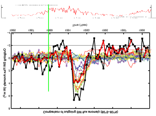
When you get everything matching up, in every nook and cranny, then you have something. And, that is what we have with the temperature and rate of change of CO2.
http://i1136.photobucket.com/albums/n488/Bartemis/nopause_zpscjndrosf.png

Tom in Florida
Reply to  Toneb
December 17, 2016 9:51 am

Toneb December 17, 2016 at 8:09 am
Tom in Florida said: “Your first graph compares absolute ppm CO2 against a temperature anomaly with a specific base period and a scale of 10ths of a degree. I suppose anyone could change either of those and produce a totally different graph that would be to their liking.”
Your reply: “Not and get the same slopes.”
But isn’t that the problem? If you changed your temperature anomaly base period to 1980-2010 and keep everything else the same, are you saying the slope of that change would be the same?

Gerald Machnee
Reply to  Toneb
December 17, 2016 4:13 pm

In the first graph, the blue does not represent temperatures prior to 100 years before present. That is part of Mann’s Trick (I would never patch proxies to thermometers). Those are proxies based on a a single tree (Bristlecone Pine) which are not true readings = faulty graph.

O R
Reply to  Duncan
December 17, 2016 4:27 am
Bartemis
Reply to  O R
December 17, 2016 9:51 am

Useless. If you plotted it against the stock market index, you would find just as great a correlation. All it tells you is they are both moving up.
Try matching every up and down movement as well as the trend, as I show above with temperature anomaly and CO2 rate of change. Now that’s a meaningful correlation!

Chimp
Reply to  O R
December 17, 2016 1:36 pm

If you plotted CO2 against temperature from 1940 to 1977, the two trend lines would not only not correlate, but move in different directions. While CO2 was rising, GASTA would be falling.
Similarly, if you plotted only from 1998 to present, CO2 would be rising while GASTA at best was flat.
So there is no correlation, except accidentally between c. 1977 and 1997.

O R
Reply to  O R
December 19, 2016 12:35 am

Yes, there are natural variations superimposed on the CO2-driven global warming signal. If you smooth them it looks like this:
http://woodfortrees.org/plot/hadcrut4gl/mean:720/plot/hadcrut4gl/mean:360/plot/esrl-co2/scale:0.0065/offset:-2.09

Bartemis
Reply to  O R
December 19, 2016 8:57 am

Utterly meaningless.

gallopingcamel
Reply to  O R
December 19, 2016 9:33 am

Bart, here is the problem with your correlation between CO2 and T: http://woodfortrees.org/plot/esrl-co2/offset:-300/trend/plot/esrl-co2/derivative
.
.
You see, the derivative removes the trend in CO2.

Bartemis
Reply to  O R
December 19, 2016 10:02 am

So what? When you integrate the derivative, you retrieve the original series.
It is not the trend in CO2 that nails temperature as the driving agent. It is the trend in dCO2/dt, which is the same as the trend in the temperature series scaled to match the variation.
http://woodfortrees.org/plot/esrl-co2/derivative/mean:24/plot/hadcrut4sh/offset:0.45/scale:0.22/from:1958/plot/esrl-co2/derivative/mean:24/trend

gallopingcamel
Reply to  O R
December 19, 2016 10:32 am

Bart all your relationship shows is that the NOISE in the CO2 signal is correlated with the temperature ANOMALY nothing else. Being that it is a mere correlation, there is no indication which variable is independent and which is dependent.

Reply to  gallopingcamel
December 20, 2016 8:27 am

gallopingcamel:
To refer to the CO2 times series as a “signal” is a mistake that results from application of terms and ideas from telecommunications to a problem in systems control. For telecommunications, the “signal” comes from the past with the result that it can travel at sub-luminal speed. For systems control, the “signal” would have to come from the future with the result that it would have to travel at super-luminal speed but the latter is impossible under relativity theory. Thus, for systems control the signal power and noise power are both nil.

gallopingcamel
Reply to  O R
December 19, 2016 10:42 am

Bart says: “you retrieve the original series.”

No, actually you do not, because when you integrate the constant of integration is arbitrary Do you remember Calc 101 ?

Bartemis
Reply to  O R
December 19, 2016 10:57 am

The variability is not “noise”, but yes, it is highly correlated between the series. So is the trend. When you scale the data to match the variability in T and dCO2/dt, you also match the long term trend (see the above link).
The argument is thereby not dependent on any assumed integration constant, or any bias offset in dCO2/dt integrating into a trend. It is based on the match between A) the variability and B) the long term trend in dCO2/dt, which integrates into a quadratic term in total CO2. Both of these components are matched by a single scaling constant. The odds of that happening by happenstance are essentially nil.

gallopingcamel
Reply to  O R
December 19, 2016 11:10 am

Bart:
.
1) You are using SH data and not global data.
.
2) You lose the absolute level of concentration of CO2 when you integrate the derivative. That’s why the constant is call ARBITRARY
..
3) You say: “The odds of that happening by happenstance are essentially nil.” and I say your correlation doesn’t prove causation. So in essence, your relationship does not tell us which variable is independent, and which is dependent. Matching two wiggly lines provides no evidence of causality.

Bartemis
Reply to  O R
December 19, 2016 12:15 pm

1) The SH data matches the satellite data best in the period of overlap, and the satellite data fit the model very, very well.
http://woodfortrees.org/plot/esrl-co2/derivative/mean:12/from:1979/plot/rss/offset:0.6/scale:0.22
The satellite data are more globally comprehensive, and not subject to the “adjustments” that have rendered the surface data suspect.
2) Doesn’t matter, as I am not hanging my hat on any arbitrary constants, but on the match of the long term trend in dCO2/dt with the trend in temperature anomaly, when the temperature anomaly is scaled to match the variation.
3) We know the direction of causality because the notion that temperature is driven by the rate of change of CO2 is absurd. Were that the case, we could see CO2 rise rapidly to very high concentration, but once it stopped, temperatures would revert to their initial values. Clearly, then, it is temperature that drives the rate of change of CO2, and not the reverse.

gallopingcamel
Reply to  O R
December 19, 2016 12:34 pm

Bart says: “We know the direction of causality” No we do not. You commit the fallacy of a false dilemma in assuming only CO2 an T are involved in the correlation. You say one side of the coin is “absurd” therefore the other side is the only alternative. There could be a third, fourth or many other factors “causing” your wiggly lines to match up .
….
You claim that ” the notion that temperature is driven by the rate of change of CO2 is absurd.” However you are not comparing temperature to the rate of change of CO2. You are comparing the temperature anomaly with the rate of change of CO2, so please address how that is “absurd.”

Bartemis
Reply to  O R
December 19, 2016 12:49 pm

Fine, if you want to split hairs:
3) We know the direction of causality because the notion that temperature anomaly is driven by the rate of change of CO2 is absurd. Were that the case, we could see CO2 rise rapidly to very high concentration, but once it stopped, temperature anomaly would revert to its initial value. Clearly, then, it is temperature anomaly that drives the rate of change of CO2, and not the reverse.
As for a separate process producing both, unlikely, but it does not matter. Either way, humans are not the major driving force.

gallopingcamel
Reply to  O R
December 19, 2016 12:55 pm

Bart says: “unlikely, but it does not matter. Either way, humans are not the major driving force.”

Hand waving extraordinaire.

Bartemis
Reply to  O R
December 19, 2016 1:05 pm

It is straightforward logic. The relationship is simply incompatible with humans being the driving force.

gallopingcamel
Reply to  O R
December 19, 2016 1:39 pm

Stop calling your “correlation” a “relationship.”

gallopingcamel
Reply to  O R
December 19, 2016 1:43 pm

Also Bart, because since your entire claim is a simple correlation, which does not show causation, you cannot logically exclude human influences.

Bartemis
Reply to  O R
December 19, 2016 1:49 pm

Yes, I can. I’ve done my best to explain why. Keep watching as events unfold.

gallopingcamel
Reply to  O R
December 19, 2016 2:36 pm

Bart says: “I’ve done my best to explain why.” Your “best” is a dismal failure. You have provided a correlation as evidence of causation. You’ committed the fallacy of false dilemma, demonstrated a lack of understanding the constant of integration, and waved your hands a lot.
.
Radiative physics offers a much more plausible causative explanation, and has evidence to support it. All you have is a couple of squiggly lines that appear to correlate.

Bartemis
Reply to  O R
December 19, 2016 4:00 pm

Sorry, no. Radiative physics suggests that temperatures might depend on absolute concentration of CO2. It does not say there is a temperature dependence on the rate of change of CO2. That would lead to absurd inferences.

gallopingcamel
Reply to  O R
December 19, 2016 4:11 pm

Bart, your correlation doesn’t explain anything. Radiative physics explains rising temperatures. Since you offer no explanation for what is actually happening in the physical world , your correlation has no value. In order to have value, you need to show a causative relationship. Try doing real science for a change.

gallopingcamel
Reply to  O R
December 19, 2016 4:13 pm

For example Bart, your correlation could be explained with a third factor, namely volcanoes. They emit both CO2 and add heat energy via the liquid lava they expel. They could be the causative explanation for the correlation of your wiggly lines.

Bartemis
Reply to  O R
December 19, 2016 4:17 pm

Again, sorry, no. The hypothesis of Earthly temperatures increasing as a function of increasing CO2 concentration does not explain why the rate of change of CO2 is proportional to temperature anomaly. You can’t square that circle.
I have offered explanations for what is happening in the real world. Scroll through the comments to find them.
And now, if you’re finished with your petty, childish insults, can we move on?

gallopingcamel
Reply to  O R
December 19, 2016 4:24 pm

I have read all of your “explanations” and I have read all of Englebeen’s rebuttals. You lose, Ferdinand wins.

Janice Moore
Reply to  O R
December 19, 2016 4:32 pm

GallopingC: You may have “read” Bartemis’ comments, but you CLEARLY have not understood them. Your own mouth condemns you,

…need to show a causative relationship…

(GC)
For all Mr. Engelbeen’s efforts (and I am not demeaning him as a scientist, per se), he has NEVER proven causation. He has a guess. That is all.
For me, and Allan MacRae and many others, Bartemis “wins,” for his argument is based on accurate, real world observation-based, data processing analysis.

Reply to  Janice Moore
December 19, 2016 11:02 pm

Janice Moore:
Mr. Engelbeen states that “empirical data conclusively reveals that CO2 has not caused temperature change over the past 38 years.” How from empirical data can Mr. Engelbeen know that CO2 has not caused this temperature change. There is no way in which Engelbeen can know this as information required for him to know this is missing.

Bartemis
Reply to  O R
December 19, 2016 4:33 pm

I will let history be the judge. The ultimate outcome really is not in doubt. This is actually a very simple and obvious problem.

gallopingcamel
Reply to  O R
December 19, 2016 4:35 pm

Bart, if you think that someone pointing out your logical fallacies, your misconception of integration, and the uselessness of your correlating the noise of two signals as “petty and childish” I feel sorry for you. Your poor little ego will be crushed if you even attempt to get a paper past peer review.

1sky1
Reply to  O R
December 19, 2016 4:36 pm

Actually, it’s not just the high correlation (or, more incisively, cross-spectral coherence) between yearly average delta CO2 and yearly temperature anomalies that points to the latter as the driver of the former. It’s the behavior of the cross-spectral phase, which shows that variations of CO2 concentration invariably LAG variations of T at frequencies of high coherence. (Unfortunately, contractual commitments prevent me from showing the actual cross-spectral results here.)
BTW, the “constant of integration” for delta CO2 is determined by the FIRST value of CO2 concentration and the actual temperature is simply the sum of the anomalies and the constant mean over the entire record. Objections of “arbitrariness” of data treatment thus are empty.

gallopingcamel
Reply to  O R
December 19, 2016 4:38 pm

Janice, all Bart has shown is a correlation. He has not shown causation. You know full well that correlation is different than causation.

gallopingcamel
Reply to  O R
December 19, 2016 4:42 pm

1sky1, ΔCO2 and dCO2 are mathematically different things, and your choice of the constant being the FIRST value is ARBITRARY

1sky1
Reply to  O R
December 19, 2016 4:51 pm

The notion that dCO2, rather than delta CO2, is at issue when dealing with digital time-series gallops far away from the manger of reality. ANY such original series can be reconstructed EXACTLY by progressively adding the partial sum of first differences to the KNOWN first value.
Merry Christmas to all, and to all a good night.

Bartemis
Reply to  O R
December 19, 2016 4:54 pm

No, GC. It is unique to match the integrated result with the original series.You were never scoring points in this regard, and you need to stop digging.

gallopingcamel
Reply to  O R
December 19, 2016 5:04 pm

1sky1, direct your comments to Bart, as he does not talk about ΔCO2 at all.
..
Look at his comments December 19, 2016 at 10:02 am, December 19, 2016 at 10:57 am, December 18, 2016 at 11:43 am, etc……

He never talks about ΔCO2, he’s talking about dCO2

Ferdinand Engelbeen
Reply to  O R
December 20, 2016 7:26 am

Bartemis:
We know the direction of causality because the notion that temperature anomaly is driven by the rate of change of CO2 is absurd.
All what you have proven is that there is a correlation between the variability of the temperature anomaly and the variability in CO2 rate of change, but that says next to nothing about the cause of the slope, because the variability and slope are proven caused by different processes.
Moreover by comparing temperature with the CO2 rate of change, you are comparing apples with oranges, as you have largely removed the origin of the slope in the CO2 rate of change: human emissions, which increased slightly quadratic over time, which gives a straight line in the derivative…
We know the direction of causality because the notion that human CO2 emissions are driven by the increase of CO2 in the atmosphere is absurd.

Ferdinand Engelbeen
Reply to  O R
December 20, 2016 8:48 am

Terry Oldberg,
Mr. Engelbeen states that “empirical data conclusively reveals that CO2 has not caused temperature change over the past 38 years.”
I never said or implied that. Empirical data do reveal that temperature can not have caused the current increase of CO2 and that humans are to blame for the bulk of the increase. That is what I said and implied…
That is supported by all available observations:
http://www.ferdinand-engelbeen.be/klimaat/co2_origin.html
That humans are the cause of the CO2 increase doesn’t imply that there will be a catastrophic increase in temperature. In my opinion only a largely benign increase which together with the increase in CO2 will be beneficial for plants all over the globe…

Bartemis
Reply to  O R
December 20, 2016 10:14 am

“…because the variability and slope are proven caused by different processes.”
They aren’t.
“…as you have largely removed the origin of the slope in the CO2 rate of change…”
The trend is clearly visible, and it matches the slope in temperature. Human emissions are not needed to provide the trend. It follows that including them in is an unnecessary complication, and a violation of Occam’s Razor.

Janice Moore
Reply to  O R
December 20, 2016 10:35 am

Dear Mr. 0ldberg,
You (unintentionlly, I realize) mistakenly attribute a quote by Mr. Dockery, the above article’s author, to Mr. Engelbeen. Lol, no wonder he made sure to pipe up! Heh. Mr. Engelbeen claims almost the exact opposite! 🙂
Re: proximate cause — it CAN be shown to be at least highly likely, i.e., not overwhelmed by another, controlling, driver.
Human CO2 emissions have NEVER been proven even “likely,” much less “highly likely” to cause a general rise in the surface temperature of the earth. It is all just a big guess (and there is anti-correlation data, now….). That CO2 has not been *conclusively* proven to lag temperature does not detract from the fact that there is much observation-based data (ice cores — with the damping equation applied) making the assertion that total atmospheric CO2 lags temperature by a quarter cycle a rational conclusion .
I think you and I largely agree, thus, some of what I wrote above was not so much directed at you as in making sure that what you wrote does not mislead someone trying to learn, here.
Thanks for taking the time to both inform and to affirm me above.
MERRY CHRISTMAS!
and HAPPY CHANUKAH!
Janice

Reply to  Janice Moore
December 20, 2016 11:41 am

Thank you for correcting my error.

Ferdinand Engelbeen
Reply to  O R
December 20, 2016 10:40 am

Bartemis:
“…because the variability and slope are proven caused by different processes.”
They aren’t.

Bart, if you don’t accept any observation, then it is a fruitless discussion. If there is anything sure in climate science , it is that more CO2 uptake by plants increases the 13C/12C ratio in the atmosphere and reverse. Thus if CO2 and δ13C change in opposite direction, plants are the main reactant.
If you have another explanation based on the literature, I am all ear.
On the other hand, the slope of dCO2/dt is NOT caused by vegetation, as that is a small, but increasing sink for CO2 over longer periods, proven by the oxygen balance and chlorophyl measurements: the earth is greening..
“…as you have largely removed the origin of the slope in the CO2 rate of change…”
The trend is clearly visible, and it matches the slope in temperature. Human emissions are not needed to provide the trend. It follows that including them in is an unnecessary complication, and a violation of Occam’s Razor.

The trend is clearly visible, as good as the trend in human emissions: about twice the trend of the CO2 increase. Occam’s Razor (and every observation) points to human emissions as cause, hardly any place for temperature…

1sky1
Reply to  O R
December 20, 2016 2:31 pm

It’s a strange Occam’s razor that totally ignores the empirically manifest cross-spectral phase between delta CO2 (which is what Bartemis is really talking about) and T in order to maintain the AGW narrative.

Bartemis
Reply to  O R
December 20, 2016 4:23 pm

“Bart, if you don’t accept any observation, then it is a fruitless discussion.”
It’s not the observations I don’t accept. It is your flimsy rationalization of what the observations mean.
“If there is anything sure in climate science , it is that more CO2 uptake by plants increases the 13C/12C ratio in the atmosphere and reverse. Thus if CO2 and δ13C change in opposite direction, plants are the main reactant.”
The second sentence does not follow from the first. It is like saying:
“If there is one thing sure in medical science, it is that viruses cause colds and colds are caused by viruses. Therefore, if you have a viral infection, you have a cold.”

Ferdinand Engelbeen
Reply to  O R
December 21, 2016 12:32 pm

1sky1,
It’s a strange Occam’s razor that totally ignores the empirically manifest cross-spectral phase between delta CO2 (which is what Bartemis is really talking about) and T in order to maintain the AGW narrative.
Not that strange: I am from the old engineering school, which was looking at the whole picture, not (only) at spectral analysis which nowadays explains “everything”.
Look at the total picture for the Mauna Loa period:
http://www.ferdinand-engelbeen.be/klimaat/klim_img/temp_co2_acc_1960_cur.jpg
There is a lot of variability in temperature, but that hardly shows up in the CO2 increase. The near perfect ratio between total human emissions and increase in the atmosphere is obvious. Between temperature and CO2 may be somewhat parallel, but with periods where there is an opposite relationship.
Now, what has Bart done: he compares the temperature with the CO2 rate of change. That is the largely detrended CO2 increase, thus he simply removed most of the increase to show that the more or less linear trend of temperature matches with the residual linear trend of the CO2 rate of change. That the latter is linear is the result of the slightly quadratic increase of CO2 in the atmosphere, obviously caused by the steady increasing accumulated human emissions. Thus Bart has effectively removed most of the cause of the CO2 increase in his comparison…
Moreover, CO2 levels go up and down with temperature with a lag, which can be seen if you enlarge the trend for both: some +/- 1.5 ppmv around the 70 ppmv trend for the extremes. That is all influence of the temperature variability and that zeroes out after 1-3 years.
Thus in fact you must compare T with CO2 and dT/dt with dCO2/dt. The latter is here:
http://www.ferdinand-engelbeen.be/klimaat/klim_img/temp_co2_der.jpg
Which makes it clear that the derivative of T has exactly the same waveform as T, but 90 degr. shifted back in time. And more important: zero slope, there is zero influence of dT/dt on the slope of dCO2/dt, only a very small offset from zero. The match of the slopes between T and dCO2/dt is completely spurious.
Why doesn’t spectral analyses give you the right answer in this case? The problem is that human emissions are all slope and very little variability, while temperature is all variability and little slope. With spectral analysis you overfocus on the variability, which in this case is not important at all for the cause of the increase…

Ferdinand Engelbeen
Reply to  O R
December 21, 2016 12:45 pm

Bartemis,
It’s not the observations I don’t accept. It is your flimsy rationalization of what the observations mean.
Bart, if you add CO2 from the oceans to the current atmosphere, then the δ13C ratio goes up. If you add CO2 from decaying vegetation, then the δ13C ratio goes down. Reverse if CO2 is absorbed by oceans or vegetation.
There is no rationalization which can change that.
The second sentence does not follow from the first.
Just handwaving without any base in isotope chemistry…

1sky1
Reply to  O R
December 21, 2016 4:55 pm

Ferdinand:
Coming from the old school of geophysical analysis, I recognize several
things that others may not:
1) The available length of record doesn’t necessarily determine any
underlying secular trend. The visual appearance of such may the result of
oscillatory signal components much longer in Fourier periodicities than the
record.
2) While spectrum analysis is by no means a panacea, it provides the most
general way of exploring the signal composition. It’s certainly far more
incisive and less limited than the primitive assumption of linear trend
plus random variability widely taught to undergraduates.
3) Non-specialists almost invariably miscomprehend the foregoing truths,
the proper methods of analysis and the potential insights provided thereby.
It’s a mistake to characterize the general effect of first-differencing as
preserving “exactly the same waveform,” while shifting the phase by a
quarter cycle. The actual transfer function is 1 – exp(iNOM), where NOM is
the normalized radian frequency, constrained to the baseband interval [-pi ,
pi]. See:
http://paloalto.unileon.es/ts/first/chapters/5fir/demos/tinvprop/fr1std.htm
It’s not really necessary–or practically possible in the strict differerntial sense that you write–to “compare T with CO2 and dT/dt with dCO2/dt.” Nor is it “the match of the slopes between T and dCO2/dt,” but the cross-spectral coherence that is of critical importance. And on that aspect of relationship between two time series, proper cross-spectrum analysis does not fail to give the right answer in any case, as you aver.
Unlike Bart’s take on the issue, it’s on the basis of the cross-spectral phase relationship between Keeling’s Mauna Loa CO2 series and a thoroughly vetted estimate of global average temperature that I dismiss CO2 as the potential driver of low-frequency variations (what you call trend)in temperature since the middle of the last century.

Ferdinand Engelbeen
Reply to  O R
December 22, 2016 11:28 am

1sky1,
I agree that it is impossible to detect a secular trend in CO2, IF that was caused by temperature, as the time period since Mauan Loa is too short.
If we can agree that ice cores are of sufficient accuracy, then Bart’s theory has a huge problem. The overall CO2/T ratio over the past 800,000 years is ~16 ppmv/K, where CO2 follows T with a variable lag: ~800 years during warming towards an interglacial and several thousands during cooling after an interglacial.
On shorter time periods, the ratio is ~5 ppmv/K (seasonal), 4-5 ppmv/K (Pinatubo, ENSO), 8 ppmv/K (MWP-LIA) and now suddenly over the past 165 years >100 ppmv/K, while humans emitted over 200 ppmv in the same time span…
The resolution of all ice cores is good enough to detect such a “spike” in the record, be it with a lower amplitude for the worst resolutions, which span the longest period.
Some more theoretical and real life comment of mine at:
https://wattsupwiththat.com/2015/11/25/about-spurious-correlations-and-causation-of-the-co2-increase-2/
It gets interesting from chapter 2.4 onwards…
With spectral analysis you have proven that dT/dt variability is the main driver for dCO2/dt variability, but as there is no slope in dT/dt, it is not responsible for the slope of dCO2/dt over time and only responsible for a small part of the increase of CO2 in the atmosphere, that is the above 4-16 ppmv/K, or about 10 ppmv of the 70 ppmv increase in the past 57 years…
Keeling’s Mauna Loa CO2 series and a thoroughly vetted estimate of global average temperature that I dismiss CO2 as the potential driver of low-frequency variations (what you call trend)in temperature since the middle of the last century.
As the time span since Mauna Loa is too short, you can’t conclude that CO2 has no influence on temperature. Anyway, I agree that the influence of CO2 on temperature is small.
My main point is reverse: the small temperature increase since Mauna Loa (or even since the LIA) can’t be the main driver of the CO2 increase in the atmosphere, only the main driver of the variability around the increase…

1sky1
Reply to  O R
December 22, 2016 5:25 pm

Ferdinand:
Not quite correct! What my cross-spectrum analysis shows is that temperature [sic!] variations are the driver of delta CO2 variations across a wide range of frequencies, including the multidecadal. This is not to say that the MEAN level of delta CO2 is driven by temperature. Indeed, the high mean level seems to be the result of human emissions, resulting in a pronounced trend in CO2 concentrations. Nowhere do I claim conversely that temperature is necessarily totally independent of CO2 levels.

Ferdinand Engelbeen
Reply to  O R
December 23, 2016 10:34 am

1sky1:
What my cross-spectrum analysis shows is that temperature variations are the driver of delta CO2 variations across a wide range of frequencies, including the multidecadal.
Seems to be quite impossible to me, as you have two possible sources for the delta CO2 over decades: human emissions and temperature.
Human emissions show a near perfect correlation with delta CO2 over the past 57 years, or even the past 116 years (including ice cores), with twice the total emissions than the increase in the atmosphere:
http://www.ferdinand-engelbeen.be/klimaat/klim_img/acc_co2_1900_cur.jpg
Compare that to the multidecadal correlation between T and CO2:
http://www.ferdinand-engelbeen.be/klimaat/klim_img/temp_co2.jpg
A change of about half the scale in temperature gives some 2 ppmv extra CO2 in the atmosphere, but 100 ppmv over the full scale? Moreover, it is proven that near all variability in CO2 is the response of vegetation to temperature variability, while vegetation is a net, growing sink for CO2 over longer periods than 1-3 years. Thus different drivers at work…
Are you sure that the attribution program doesn’t attribute the multidecadal increase to the wrong variable?
Again the main problem may be in the fact that human emissions may have too little variability: that isn’t even detectable at Mauna Loa (less than 0.2 ppmv after half is absorbed by oceans and vegetation).

1sky1
Reply to  O R
December 23, 2016 1:00 pm

Ferdinand:
My attribution is certainly not to the wrong variable. You have to understand that the relationship at issue here is not what you show, but that between the yearly DELTA CO2 and T, akin to what was shown here bycomment image.
In proper cross-spectrum analysis the mean of both variables is removed, leaving only the VARIATIONS about the respective means. It turns out that the r.m.s. variations of delta CO2 are of the same order as the mean. While I attribute the sizable mean of delta CO2 to human emissions, the cross-spectral phase of the variations manifest by the data permits only the attribution of temperature variations as the driver of delta CO2 variations, not the other way around. You can’t have the putative physical driver lagging the response.

1sky1
Reply to  O R
December 23, 2016 1:27 pm

It should be stressed that I used Keeling’s Mauna Loa CO2 series along with a proprietary, vetted estimate of GAST; my cross-spectral findings thus are restricted to the time period 1958 onward. Also, to be entirely punctilious, it’s not that DELTA CO2 variations per se lag behind T variations that is the basis of my attribution. It’s that the residual CO2 variations [sic!] would lag behind measured T variations during that period.

Ferdinand Engelbeen
Reply to  O R
December 23, 2016 1:53 pm

1sky1,
I think that we largely agree that the variability in delta CO2 is caused by the variability of temperature, not the opposite way and that most of the offset of 1-3 ppmv/annum is caused by human emissions.
There may be a secular slope in CO2 caused by temperature, but that is maximum 16 ppmv/K per Henry’s law. Maybe you can use the longer time frame of two out of three Law Dome ice cores (DE08 and DE08-2) to expand the time period of interest to 150 years back in time, even when the CO2 data are smoothed over a period of ~8 years and are less accurate (~1.2 ppmv, 1 sigma) than Mauna Loa for the secular slope…
Still that doesn’t exclude a small influence of the increased CO2 level on temperature…

Reply to  Duncan
December 17, 2016 6:36 am

Duncan, pray do not be so silly. If one changed the temperature scale to -1 to +1, say, then the temperature trace would shoot up precipitously and career off-scale by 1995 – which wouldn’t be very useful. You could certainly change the scale to -1 to +20, say, in order to force the gradients to look similar but then you would simply have yards of y axis doing nothing which wouldn’t be very useful – or honest – either.

Duncan
Reply to  cephus0
December 17, 2016 10:38 am

Sure 1998 would go off scale. This graph was just one data set. Combine it will 100’s of others, average it, smooth it, pound it into submission, then scale it to match two slopes, then and only then will you receive your grant money.
I was just making a point the graph had suspicious scaling, the same trick used by warmists.

Reply to  cephus0
December 17, 2016 12:28 pm

The period from 1980 to present has shown a warming trend.
Which is said to be disastrous and the cause of all manner of future ills.
Prior to 1980, the trend was cooling for over 30 years.
Which was said at the time to be disastrous and the cause of all manner of future ills.
Interestingly, many of the claimed disastrous effects of both are identical!
It is a good thing it warmed up some…worldwide conditions for growing food and general survival have been improving.
It was durn cold in the 1970s!
Hey, how many people are going planning to spend some vacation time this winter in the polar regions, and how many are hoping and/or planning to visit places closer to the equator?

Alan McIntire
Reply to  Duncan
December 17, 2016 3:24 pm

As Bevan Dockery pointed out, the correlation between the two, temperature and CO2 is very high BEFORE detrending, so the pictue graph is irrelevant here.
Take a series of 30 coin tosses, counting heads as plus 1 and tails as minus one and keep a running total.
Do the same for a second series of 30 coin tosses and you’re likely to get a correlation close to + or – 1.

Reply to  Duncan
December 17, 2016 5:56 pm

If one changed the temperature scale say from -1 to +1

Why is the temperature, in that chart not give in ºK? The CO2 scale is in ppm and starts at zero. So should temperature start at its absolute zero. This obsessive cherry picking of temperature ranges and, especially, time periods, leaves me deeply distrustful.

stan robertson
December 16, 2016 6:27 pm

A physicist, Lon Hocker, showed that a chord derivative of CO2 concentration vs time showed spikes that identified every El Nino back into the 1950s. It was posted here on WUWT some years ago, but I can’t find it at the moment.

Stephen Singer
December 16, 2016 6:35 pm

Where’s the red montly CO2 concentration line in Figure 2?

TonyL
Reply to  Stephen Singer
December 16, 2016 7:15 pm

It is there, for sure. The red is overdrawn, on the heavy black line. If you open the graph in a new window and embiggen, you can see it a bit better. Sometimes the graphics do not translate and render as cleanly as we would like.

December 16, 2016 6:46 pm

Here is 38 years of empirical data clearly showing a relationship between the satellite temperature and the rate of change of atmospheric CO2 concentration at the Mauna Loa Observatory.

False. Plotting two datasets can never show a relationship between them. Correlation does not imply a relationship.
The relationship between rate of change in CO2 and temperatures is known since the late 70’s and has been satisfactorily explained. It has been discussed here at WUWT thousands of times. It is related to the sinks response to temperature and has nothing to do with the long term trend in CO2 or temperatures. I suggest better documentation next time.

Chimp
Reply to  Javier
December 16, 2016 6:51 pm

Well spoken. Like a true man of science. Or person thereof.

Reply to  Javier
December 16, 2016 8:57 pm

You must have missed THIS statement later:
“Here again is 38 years of empirical data, this time showing a distinct lack of a relationship between the satellite temperature and the atmospheric CO2 concentration.”

Hugs
Reply to  Aphan
December 16, 2016 11:52 pm

And that part is just untrue.

Reply to  Aphan
December 17, 2016 7:50 am

As it should be since the expected dependence is logarithmic, how many times more are we going to see junk graphs like Fig 2 posted on here. Let’s have some honesty and plot log(CO2).

Bartemis
Reply to  Javier
December 17, 2016 9:55 am

“… and has been satisfactorily explained.”
No, it hasn’t. In the late 70’s, there were not enough data to show that both the short term variation and the long term trend match.
It’s just been buried in a bunch of hand waving, not explained, let alone satisfactorily.

Reply to  Bartemis
December 17, 2016 10:27 am

Yes it has. Very conclusively. Bacastow studies allowed to elucidate the role of oceanic currents and vegetation on the seasonal CO2 cycle.
Bacastow, R. B. “Modulation of atmospheric carbon dioxide by the Southern Oscillation.” Nature 261 (1976): 116-118.
Bacastow, R. B., C. D. Keeling, and T. P. Whorf. “Seasonal Amplitude Increase in Atmospheric Concentration.” Journal of Geophysical Research 90.D6 (1985): 10-529.
The correspondence between the first derivative of atmospheric CO2 levels and temperatures is due to sinks response to temperatures. This issue has been beaten to death at WUWT and every other climate site. Everybody with a minimum knowledge at both sides of the debate agrees. It has nothing to do with global warming and it is a telltale for skeptics that haven’t done due diligence on their beliefs.

Bartemis
Reply to  Bartemis
December 18, 2016 11:08 am

Nonsense. Vegetation is not producing the long term trend.
The entire record of CO2 change in the modern era can be reproduced from the temperature data only to high fidelity using a simple, affine parameterization. It is idiotic to imagine that, that is mere happenstance.

Ferdinand Engelbeen
Reply to  Bartemis
December 21, 2016 12:55 pm

Bartemis,
Nonsense. Vegetation is not producing the long term trend.
Indeed, but vegetation IS producing near all variability. That is the problem with your theory… Mathematically still possible, but trend and slope are not caused by the same processes…

DWR54
Reply to  Javier
December 17, 2016 2:52 pm

Javier
“Correlation does not imply a relationship.”
____________
True, but where there is known causative effect, then correlation is evidence supporting a proposition.
CO2 is a greenhouse gas that should, with associated feedbacks such as increased water vapour and reduced sea ice cover, force climate in a warming direction. The causative effect of CO2 should be to increase temperatures at the surface and lower atmosphere.
When all the world’s data sets, including satellite data sets, show a long term correlation between CO2 and global temperature increase, that doesn’t ‘prove’ correlation; but it is certainly evidence supporting the theory that CO2 is contributing to warming the atmosphere.

Gerald Machnee
Reply to  DWR54
December 17, 2016 4:26 pm

Re DWR54
**CO2 is a greenhouse gas that should, with associated feedbacks such as increased water vapour and reduced sea ice cover, force climate in a warming direction. The causative effect of CO2 should be to increase temperatures at the surface and lower atmosphere.**
There is no proven feedback from increased water vapor. Increased water vapor results in more cloud which reflects solar radiation resulting in cooling. YUour causative effect is an unproven theory.
.
**When all the world’s data sets, including satellite data sets, show a long term correlation between CO2 and global temperature increase, that doesn’t ‘prove’ correlation; but it is certainly evidence supporting the theory that CO2 is contributing to warming the atmosphere.**
The correlation is not very good, but NASA/NOAA are trying to make it better by adjusting the temperatures – note the graph posted above, as well as:
http://realclimatescience.com/alterations-to-climate-data/
It is not evidence, but only one thing to look at. There is too much annual and monthly variation in the temperatures to be caused by CO2. There are many other factors being considered such as changes in solar radiation , magnetism, changes in cloud and moisture.

Reply to  DWR54
December 17, 2016 5:39 pm

True, but where there is known causative effect, then correlation is evidence supporting a proposition.

I accept that. But in this case causation works both ways. CO2 increases temperatures and temperatures increase CO2. However we know from the past that there is no runaway effect so feedbacks MUST be net negative or less than 1.
In the end we don’t know how much warming the increase in CO2 has caused, but since the 1910-1945 warming and the 1975-2000 warming are not very different while the CO2 difference is big, this suggests that CO2 warming, although noticeable, is not overpowering. The pause is also evidence that CO2 warming can be counteracted fully by natural forcings and variability.
And we have very strong evidence that warming was here before there was any change in CO2.
http://i.imgur.com/fa9yhHJ.png
So yes, CO2 surely warms, but no, that does not appear to be a problem. There is a very good chance that half or more of the warming is natural.

Berniea
December 16, 2016 7:07 pm

So many ignorant comments from ignorant people. This is a excellent piece of work and should be published. You can see the blips in CO2 coincident with the El Ninos. This work quantifies the relationship over short time periods.

NZ Willy
Reply to  Berniea
December 16, 2016 7:41 pm

Agreed it should be published,

Reply to  Berniea
December 16, 2016 7:47 pm

Berniea,
Unfortunatey the climatists are well aware of the ENSO – d(pCO2)/dt relationship.
But like the fact that 2015 and (likely) 2016 are the warmest years (in GISStemp) solely due to a major ElNino is a detail that gets lost in the communication to the public.

tony mcleod
Reply to  Joel O’Bryan
December 17, 2016 3:36 am

“solely due to a major ElNino”
Untrue, and obviously untrue with little more than a cursory glance at the graph. The last three major El ninos have been overlaying a background rise in temperature. So despite the 1998 El nino actually being a little stronger than 2015, the recent peak was higher. “solely” is incorrect.

Chimp
Reply to  Joel O’Bryan
December 17, 2016 3:39 pm

Tony,
Whatever slight rise in background temperature may actually have occurred since the PDO flip of 1977 cannot be attributed to an increase in CO2. So many variables underlie such a small increase in global average warmth that any effect from CO2 “forcing” (man-made or not) must be too small to measure, even with assumed feedback effects.

Chimp
Reply to  Joel O’Bryan
December 17, 2016 3:40 pm

Which is but one reason why the GIGO models have failed so epically.

Hugs
Reply to  Berniea
December 17, 2016 12:03 am

I’m agreeing on ignorance.

December 16, 2016 7:37 pm

Good work Bevan
Humlum et al and you should kindly cite my originating paper of Jan2008 at
http://icecap.us/index.php/go/joes-blog/carbon_dioxide_in_not_the_primary_cause_of_global_warming_the_future_can_no/

December 16, 2016 7:41 pm

340 W/m^2 ISR arrive at the ToA (100 km per NASA), 100 W/m^2 are reflected straight away leaving 240 W/m^2 continuing on to be absorbed by the atmosphere (80 W/m^2) and surface (160 W/m^2). In order to maintain the existing thermal equilibrium and atmospheric temperature (not really required) 240 W/m^2 must leave the ToA. Leaving the surface at 1.5 m (IPCC Glossary) are: thermals, 17 W/m^2; evapotranspiration, 80 W/m^2; LWIR, 63 W/m^2 sub-totaling 160 W/m^2 plus the atmosphere’s 80 W/m^2 making a grand total of 240 W/m^2 OLR at ToA.
When more energy leaves ToA than enters it, the atmosphere will cool down. When less energy leaves the ToA than enters it, the atmosphere will heat up. The GHE theory postulates that GHGs impede/trap/store the flow of heat reducing the amount leaving the ToA and as a consequence the atmosphere will heat up. Actually if the energy moving through to the ToA goes down, say from 240 to 238 W/m^2, the atmosphere will cool per Q/A = U * dT. The same condition could also be due to increased albedo decreasing heat to the atmosphere & surface or ocean absorbing energy.
The S-B ideal BB temperature corresponding to ToA 240 W/m^2 OLR is 255 K or -18 C. This ToA “surface” value is compared to a surface “surface” at 1.5 m temperature of 288 K, 15 C, 390 W/m^2. The 33 C higher 1.5 m temperature is allegedly attributed to/explained by the GHE theory.
BTW the S-B ideal BB radiation equation applies only in a vacuum. For an object to radiate 100% of its energy per S-B there can be no conduction or convection, i.e. no molecules or a vacuum. The upwelling calculation of 15 C, 288 K, 390 W/m^2 only applies/works in vacuum.
Comparing ToA values to 1.5 m values is an incorrect comparison.
The S-B BB ToA “surface” temperature of 255 K should be compared to the ToA observed “surface” temperature of 193 K, -80 C, not the 1.5 m above land “surface” temperature of 288 K, 15 C. The – 62 C difference is explained by the earth’s effective emissivity. The ratio of the ToA observed “surface” temperature (^4) at 100 km to the S-B BB temperature (^4) equals an emissivity of .328. Emissivity is not the same as albedo.
Because the +33 C comparison between ToA “surface” 255 K and 1.5 m “surface” 288 K is invalid the perceived need for a GHE theory/explanation results in an invalid non-solution to a non-problem.
References:
ACS Climate Change Toolkit
Trenberth et. al. 2011 “Atmospheric Moisture Transports …….” Figure 10, IPCC AR5 Annex III
http://earthobservatory.nasa.gov/IOTD/view.php?id=7373
http://principia-scientific.org/the-stefan-boltzmann-law-at-a-non-vacuum-interface-misuse-by-global-warming-alarmists/
http://earthobservatory.nasa.gov/IOTD/view.php?id=7373
340 – 100 albedo = 240. Albedo is out of the equation so 240 ISR and 240 OLR are left to work out the balance.

December 16, 2016 7:46 pm

https://wattsupwiththat.com/2015/06/13/presentation-of-evidence-suggesting-temperature-drives-atmospheric-co2-more-than-co2-drives-temperature/
Observations and Conclusions:
1. Temperature, among other factors, drives atmospheric CO2 much more than CO2 drives temperature. The rate of change dCO2/dt is closely correlated with temperature and thus atmospheric CO2 LAGS temperature by ~9 months in the modern data record
2. CO2 also lags temperature by ~~800 years in the ice core record, on a longer time scale.
3. Atmospheric CO2 lags temperature at all measured time scales.
4. CO2 is the feedstock for carbon-based life on Earth, and Earth’s atmosphere and oceans are clearly CO2-deficient. CO2 abatement and sequestration schemes are nonsense.
5. Based on the evidence, Earth’s climate is insensitive to increased atmospheric CO2 – there is no global warming crisis.
6. Recent global warming was natural and irregularly cyclical – the next climate phase following the ~20 year pause will probably be global cooling, starting by ~2020 or sooner.
7. Adaptation is clearly the best approach to deal with the moderate global warming and cooling experienced in recent centuries.
8. Cool and cold weather kills many more people than warm or hot weather, even in warm climates. There are about 100,000 Excess Winter Deaths every year in the USA and about 10,000 in Canada.
9. Green energy schemes have needlessly driven up energy costs, reduced electrical grid reliability and contributed to increased winter mortality, which especially targets the elderly and the poor.
10. Cheap, abundant, reliable energy is the lifeblood of modern society. When politicians fool with energy systems, real people suffer and die. That is the tragic legacy of false global warming alarmism.
Allan MacRae, Calgary, June 12, 2015

December 16, 2016 7:46 pm

“It follows that this synthesis of empirical data conclusively reveals that CO2 has not caused temperature change over the past 38 years but that the rate of change in CO2 concentration may have been influenced to a statistically significant degree by the temperature level.”
The second is true, a short-term effect, and no surprise. When oceans warm, they emit CO2. When they cool, it goes back again. No-one doubts that.
The first is false, and does not follow. No-one claims that the rate of CO2 change, as in Fig 1, causes warming. What the IPCC claims is that, on a much longer time scale than these wiggles, CO2 retains heat and an increased level causes warming. That is a slow effect; the post-industrial forcing is of order 2 W/m2. That won’t do anything observable in a year, but is inexorable. That is why your plot, even the cherrypicked tropospheric tropical land only, still rises over the period.

Reply to  Nick Stokes
December 16, 2016 8:10 pm

Nick,
my money is on the Climate Hustlers, from Steyer to Gavin, will need to find a new hustle by 2022.
Steyer (and his ilk Soros) will be okay since they have billions banked as cash. Gavin will probably need to emigrate to Canada or NZ if he wants to keep his personal gravy train rolling.

Robert from oz
Reply to  Nick Stokes
December 16, 2016 8:29 pm

Longer time scales nick ? How far back do you want to go , when Co2 was up and temps were down or not quite that far to suit your religion.
Keep the faith you troll , keep the faith .

Owen Suppes
Reply to  Robert from oz
December 17, 2016 11:36 pm

Robert, calling Nick a troll doesn’t improve your grasp of radiative physics.

Frank Karvv
Reply to  Nick Stokes
December 16, 2016 10:48 pm

So no CO2 logarithmic decreasing effect according to NS. Just an “inexorable” constant rise over time??
Inexorable: unyielding or unalterable. If CO2 has a decreasing effect as it would have over time then its influence is alterable.

Nick Stokes
Reply to  Frank Karvv
December 16, 2016 11:38 pm

I didn’t say constant. But the currently increasing would anyway outweigh the logarithmic effect.

Ian W
Reply to  Frank Karvv
December 17, 2016 1:46 am

But the currently increasing would anyway outweigh the logarithmic effect.

Surely the opposite is true; the effect of each doubling halves until the effect is unmeasurably small and therefore imperceptible.

hunter
Reply to  Frank Karvv
December 17, 2016 3:48 am

The logarithmic effect is not a step function. It is constant.

Hugs
Reply to  Nick Stokes
December 17, 2016 12:04 am

Thanks Nick.

Brett Keane
Reply to  Nick Stokes
December 17, 2016 2:06 am

@fNick Stokes
December 16, 2016 at 7:46 pm:
If it is not instantaneous, it does not exist, Nick. Being supposedly radiation. One day you might learn that radiation is an effect not a cause. But probably you will never comprehend what that means. Too much like Physics, beautiful stuff that it is.

azeeman
Reply to  Brett Keane
December 17, 2016 12:07 pm

Physics and climate “science” don’t intersect. The concept of an average temperature doesn’t exist in physics. Physics also relies on traceability. If a voltage measurement is in dispute, the instruments used to measure it the voltage can be traced back to a lump of metal in Paris. The concept of traceability doesn’t exist in climate science. Everything is based on some dubious statistics with no traceability, endless adjustments and parameters (e.g. wooden versus steel buckets) and never ending disputes because of the lack of traceability.
No sane person would trust a climate “scientist” to send a man to the moon or even run a lemonade stand. Without a solid scientific basis that stands without argument, climatology is at the same level as homeopathy and astrology.
Einstein’s theory of gravity superseded Newton’s only when very high precision, repeatable and traceable measurements showed flaws in Newton’s theory. The high precision of modern GPS relies on Einstein not Newton. Predictions can be made and tested with extremely high precision such as the recent discovery of gravity waves.
Climate predictions other than seasonal such as winter will be colder than summer are possible, but predictions of any precision are impossible or untestable.

catweazle666
Reply to  Brett Keane
December 17, 2016 6:54 pm

“climatology is at the same level as homeopathy and astrology.”
THAT good?
I seriously doubt it!

hunter
Reply to  Nick Stokes
December 17, 2016 3:47 am

Nick, people do claim that CO2 increases manifest as so-called “extreme weather” today. Please don’t be so dismissive.

Reply to  Nick Stokes
December 17, 2016 6:37 pm

“CO2 retains heat”
Actually a good description of what it does, since it has an absorptivity of nearly 1 and an emissivity of .002. The whole “radiative” part of the “forcing” is off track, and this applies to Willis’ downwelling work at AGU. You cannot infer radiation from absorption for CO2 except by multiplying by .002. Out of 500 photons absorbed, 1 is emitted. The other 499 quanta are dissipated kinetically.
CO2 cannot warm the 95% of the atmosphere that is transparent in the CO2 bands by radiation. It must do it kinetically, and it does. Just not very much. The fundamental CO2 band extinguishes all earthlight at 280 ppm. Additional gas cannot absorb more light because there isn’t any (more light). The remaining unsaturated CO2 bands where earthlight is not yet extinguished, are one order to many orders of magnitude weaker.

Reply to  gymnosperm
December 18, 2016 3:52 am


Could you help me out. I’m pretty convinced CO2 actually has a (small) cooling effect.
During daytime solar IR is absorbed by CO2 near 2000 nm.
https://en.wikipedia.org/wiki/Sunlight#/media/File:Solar_spectrum_en.svg
This means that a little less solar is reaching the surface than without CO2 => cooling effect.
During night time the surface cools,
How fast is the day time solar energy “stored” in the CO2 molecules lost to the surrounding atmosphere or directly to space.
I do assume a CO2 molecule “excited” to its max by solar is not able to be even more excited by the much weaker surface radiation.

Reply to  Ben Wouters
December 18, 2016 9:07 am

I don’t know much about the near IR CO2 absorption at about 2000 nm/WN 5000. In a quick search I can’t even find the excitation mode. H2O may overlap, but the net effect seems to be complete absorption at those wavelengths.
Whether the net effect is warming or cooling is also hard to know. This is “top down” so the higher the altitude of complete absorption, the greater the chance of a cooling effect.

Reply to  Ben Wouters
December 19, 2016 7:16 am

The absorption peaks at 2013 and 2060 nm are v3 asymmetric stretches. They work in the mesosphere.
http://jvarekamp.web.wesleyan.edu/CO2/FP-1.pdf

Reply to  gymnosperm
December 20, 2016 8:15 am


Thanks for the link. So CO2 in the mesosphere intercepts solar IR around 2000nm and prevents it from reaching the surface (and heats the mesosphere)
Can the other absorption bands of CO2 do the same in the troposphere?
That is heat the troposphere during daytime, and radiate to space during the night.
I’m trying to get a feel for the mechanism that results in the troposphere temperature profile to shift roughly 1K from day to night and back. The surface cools much faster (and cools the lower few 100 meters atmosphere with it) since it can radiate directly to space (atmospheric window).
(I think I have uncovered the mechanism that explains our very high surface temperatures. (>90K higher than the moons) Role of the atmosphere is just slowing the energy loss to space. No warming of the surface required)

Reply to  Ben Wouters
December 22, 2016 8:17 am

In the fundamental bend at wave number 667.4 and rotations, CO2 has an absorption coefficient of nearly 1 and an emissivity of .002. Back radiation of the surface is thus very small as you suggest. Back, forth, and every which way radiation is essentially nonexistent below 300 meters in these bands.

Reply to  gymnosperm
December 23, 2016 5:57 am

December 22, 2016 at 8:17 am
“Back, forth, and every which way radiation is essentially nonexistent below 300 meters in these bands.”
I assume this is because the density is too high, and it’s mostly collisions that provide energy transfer?
(and evaporation near the surface)
To me this also means that during daytime it is mostly solar IR that is intercepted by predominantly H2O and a little by CO2. Surface IR is too weak then to matter much.

Reply to  Ben Wouters
December 23, 2016 8:46 am

Yes, pressure broadening of the lines, the very short (1 meter) extinction path, and the very low emissivity combine to ensure the dominance of kinetic dissipation of the energy absorbed by CO2 at 667.4 (15 microns) below 300 meters.
Water absorbs a ton of near IR top down from the sun, and it does it in the lower troposphere where most of the water is. If you look at Trenberth’s energy budget you will see 23% of TSI absorbed by the atmosphere. That’s 78 watts (an incandescent bulb) for every square meter. Oddly, this is ignored in the quibbling over a couple watts of “back” radiation.
Water radiates as a blackbody to a much higher altitude than CO2, not showing much deviation from the Planck curve until about three kilometers. Water has no “Q” branch and experiences mostly rotational transitions. Below three kilometers its influence on atmospheric temperature is kinetic (not radiative) as well.

Reply to  gymnosperm
December 27, 2016 8:01 am

December 17, 2016 at 6:37 pm
” If you look at Trenberth’s energy budget you will see 23% of TSI absorbed by the atmosphere.”
This whole backradiation idea (about twice as much backradiation as solar radiation) seems physically impossible to me. Unless I see a working backradiation panel harvesting this energy I can’t accept it as reality.
This diagram gives a more realistic energy budget:comment image
We only have to explain how the surface got to ~290K.
Simple answer: by cooling down.
https://tallbloke.wordpress.com/2014/03/03/ben-wouters-influence-of-geothermal-heat-on-past-and-present-climate/

December 16, 2016 7:52 pm
Reply to  Michael Scott
December 17, 2016 4:25 am

Yes, there is actually a lag of 7 months between the temperature change to when the CO2 changes occur.
One issue to be careful with though, is that there are seasonal adjustments in the data for both temperature and CO2. When you are careful with that by looking at the numbers both seasonally adjusted and not seasonally adjusted, there is still a lag of 5 to 9 months but it gets harder to see.

Bartemis
Reply to  Bill Illis
December 17, 2016 9:59 am

No, there is no fixed time lag. It is frequency dependent, and with a phase lag of a fixed 90 deg.

Vlad the Impaler
Reply to  Bill Illis
December 17, 2016 2:57 pm

Completely off-topic:
Mr. Illis: Jo Nova [is/may be] trying to contact you. The generic e-mail is “support (at) joannenova (dot) com (dot) au”
No quotes in the above; ref: 750 m.a. T vs. CO2

Reply to  Michael Scott
December 17, 2016 4:57 pm

Michael Scott December 16, 2016 at 7:52 pm
“Comparison between CO2 and Temp from 1960 on showing Temp proceeding CO2 http://www.woodfortrees.org/graph/esrl-co2/mean:12/scale:0.2/isolate:60/plot/hadcrut4gl/isolate:60/mean:12/from:1961
I do not know what you were doing here. you used to isolate 60 months and than you used a mean of 12 months to the result of it.
I checked at WFT what isolate means and got the answer:
Does the same running mean as ‘mean’, but then subtracts this from the raw data to leave the ‘noise’
Still I’m stepping in the dark…

December 16, 2016 7:59 pm

Sorry I really prefer when people post, that they do not just put up a graphic. Here is a link to the web site, so you can play with the image. http://www.woodfortrees.org/plot/esrl-co2/mean:12/scale:0.2/isolate:60/plot/hadcrut4gl/isolate:60/mean:12/from:1961

pochas94
December 16, 2016 8:44 pm

One must remember that the correlation coefficient between two straight lines is always 1 (or minus 1) whether they have the same slope or not. For such a coefficient to be meaningful both sets of data must include all of the variability. For a record with variability on seasonal, decennial, centennial, and millennial scales, like climate, these short term correlation coefficients have little meaning.

Bartemis
Reply to  pochas94
December 17, 2016 10:01 am

Exactly! These graphs showing temperature and CO2 vaguely marching in the same direction are meaningless. A significant correlation looks like this:
http://i1136.photobucket.com/albums/n488/Bartemis/nopause_zpscjndrosf.png

December 16, 2016 8:49 pm

You should get in the habit of squaring reported correlation coefficients whenever you see them in publications, to determine the actual strength of the relationship (also known as the coefficient of determination).
People who haven’t been educated in mathematical statistics may naively assume that a correlation coefficient of r = .50 means that the relationship accounts for half of change in the dependent variable. However, “The strength of the relationship between X and Y is sometimes expressed by squaring the correlation coefficient and multiplying by 100. The resulting statistic is known as variance explained (or R^2). Example: a correlation of 0.50 means 0.5^2 x 100 = 25% of the variance in Y is “explained” or predicted by the X variable.” http://sportsci.org/resource/stats/correl.html
That means a correlation of r < 0.50 or < 0.40 has very little explanatory value even if the data are NOT from autocorrelated time series. Values in that range are essentially meaningless, as discussed above, If the data are from autocorrelated time series (most are). In other words, garbage in, garbage out.

jim heath
December 16, 2016 8:54 pm

For the novices I will simplify all of the above on Global Warming: It’s crap.

Reply to  jim heath
December 16, 2016 8:59 pm

Lol! Bravo!

Hugs
Reply to  jim heath
December 17, 2016 12:07 am

But for different reason than stated above.

December 16, 2016 9:08 pm

Regarding: “it is possible that the almost 2 ppm per annum increase in CO2 concentration over the past 38 years has arisen from biogenetic sources driven by the natural rise in temperature following the last ice age.” In previous comings and goings of ice age glaciations, CO2 varied around or a little over 10 PPM per degree C temperature change. We’re now around 120 PPM above typical ionterglacial values. Also, the global carbon budget is known well enough for it to be known that in the past several decades, nature has been a net sink, removing nearly half of anthropogenic CO2 emissions so far.

Bartemis
Reply to  Donald L. Klipstein
December 17, 2016 10:03 am

“…nature has been a net sink, removing nearly half of anthropogenic CO2 emissions so far.”
(Sigh) The ridiculous pseudo-mass balance argument again. Nature, minus its dynamic response to anthropogenic forcing is not a net sink. This is a dynamic system. Static bookkeeping does not apply.

Ferdinand Engelbeen
Reply to  Bartemis
December 21, 2016 1:16 pm

Bartemis:
Nature, minus its dynamic response to anthropogenic forcing is not a net sink.
Of course nature is a net source and human emissions simply disappear into space…
No matter what causes the increase in the atmosphere, natural sinks react equally to any CO2, whatever the source, above steady state. Thus either the natural cycle didn’t change much over time and (near) all extra CO2 is from humans, or the natural cycle increased a fourfold in lockstep with the fourfold increase of human emissions, or you can’t have a fourfold increase rate in the atmosphere and net sink rate…

December 16, 2016 9:15 pm

Regarding: “Note that it is not possible for a rise in CO2 concentration to cause the temperature to increase and for the temperature level to control the rate of change of CO2 concentration as this would mean that there was a positive feedback loop causing both CO2 concentration and temperature to rise continuously and the oceans would have evaporated long ago.” Feedback can be positive but short of causing runaway. Zero feedback means a feedback factor of zero. A feedback factor of 1 is borderline runaway. A feedback factor between zero and 1 is positive feedback short of runaway. Increasing temperature causes increase of CO2, and increase of CO2 causes increase of temperature. There is positive feedback with a feedback factor less than 1.

December 16, 2016 9:28 pm

The satellite temperature plot in Figures 1 and 2 is not global temperature but temperature of the lower troposphere over tropical land. I suspect that was chosen because there the 1997-1998 El Nino spike is dominant to an outlier extent and the spike of the recent El Nino is notably small. In global temperature, these two El Ninos had similarly tall spikes.

Richard M
Reply to  Donald L. Klipstein
December 17, 2016 5:53 am

Keep in mind the latest El Nino spike is enhanced by the loss of Arctic sea ice driven by the AMO. If you just look at the tropics you minimize the AMO’s influence.

Bindidon
Reply to  Donald L. Klipstein
December 17, 2016 4:29 pm

Donald L. Klipstein on December 16, 2016 at 9:28 pm
Here is a comaprison of UAH6.0beta5 for
– the Globe (blue);
– the Tropics (red);
– the Nino3+4 area (green).
http://fs5.directupload.net/images/161215/86mdzjx7.jpg
You see that ENSO 2015/16 is higher than ENSO 1997/98 for the Globe, and that the inverse holds for the Tropics.

December 16, 2016 9:36 pm

Stop showing off how smart you are in statistics. I do not want to know about the Durbin-Watson test or whether ordinary linear regression is applicable or not. Dump your first four paragraphs and rewrite them in English. I can see without memorizing sixteen numbers that the main peaks in figure 1 coincide. Explain that without all the statistical babble.

Mary Brown
Reply to  Arno Arrak (@ArnoArrak)
December 17, 2016 8:47 am

Agreed. Less stat-babble would be good. And I do stats every day.

John Harmsworth
Reply to  Mary Brown
December 17, 2016 12:02 pm

I hear that! If some of these people were on fire they’d be arguing how much of the temp was due to the flu or their earlier work out. It all smacks of an utterly unproven theory, like calculating how many angels
( Christmas thought) exhale how much CO2.

Reply to  Mike McMillan
December 16, 2016 10:03 pm

“Dr Murry Salby was saying a couple years ago”
and which we still can’t see written down anywhere.

Robert from oz
Reply to  Nick Stokes
December 16, 2016 11:11 pm

Nick , what was your religion saying a couple of years ago ?
More acidic oceans.
End of the world if Co2 levels were not lowered .
20 ft sea rise .
Want me to stop with facts you dim witted bird brain troll ?

Hugs
Reply to  Nick Stokes
December 17, 2016 12:10 am

And which don’t make sense anyway. I’m sorry to be so blunt, but Salby is talking all bonkers.

Hugs
Reply to  Nick Stokes
December 17, 2016 12:15 am

And Robert, quote exact words as Willis says and keep on topic, please.

Robert from oz
Reply to  Nick Stokes
December 17, 2016 12:21 am

Ahh hugs a new troll or maybe old shamed one with new Monica , whatever .
Your Darling troll Nick did specify “a couple of years ago ” or am I reading that wrong ? If indeed he does say a couple of years , what’s the problem ? Troll !

Toneb
Reply to  Nick Stokes
December 17, 2016 4:06 am

“More acidic oceans.
End of the world if Co2 levels were not lowered .
20 ft sea rise .
Want me to stop with facts you dim witted bird brain troll ?”
The only one of those that is a “fact” is that the oceans are becoming more acidic.
The other two are NOT facts.
Oh – there is one other.
Nick provides science.
That you do not agree with it does not make him a Troll.
People who flame others via hand-waving and zero evidence are Trolls.
Nick is too polite to say that – so I will.
Oh, and would denizens really like a pure echo-chamber here?

Clyde Spencer
Reply to  Nick Stokes
December 17, 2016 10:35 am

ToneB,
If I were to say that “You have become more agitated,” would it be correct if you weren’t agitated to begin with? If a measurement changes from 8 to 7, would it be correct to say it has become more negative? The oceans are NOT acidic, and probably never will be. Therefore, any claim that they are “becoming more acidic” is disingenuous. It is NOT a fact. It is a willful attempt to influence people’s thinking with a non-fact.

Freedom Monger
Reply to  Nick Stokes
December 17, 2016 10:36 am

No Toneb, it is exactly the opposite.
I see, time after time, the scientists here obliterate every argument Nick and you make.
Because of the empirical evidence and science presented here, I am thoroughly convinced that CO2 generally follows Temperature and doesn’t drive it.
This indicates that those who advocate Policy to restrict CO2 emissions have an agenda other than “saving the planet”, because their efforts and their solutions will do nothing of the sort.
Outside, the only ones I see that would truly benefit from the proposed Climate Policies are those who crave the institution of a certain kind of Power and Dominion.
I abhor ad hominem attacks. A Winner doesn’t make them.
While you and Nick can and do make some cogent arguments, you are losing. You are losing because you are advocates for Policy rather than Science. When all your scientific verbiage is stripped away your ultimate Message is that everyone needs to be Afraid and accept the Solutions of the Powers that be.
If you were really Advocating the Science, even with the positions you hold, you would logically and rationally have to say, “The Earth is Warming? Man is causing it? So what – it’s not really a Problem.)
We are a long, long, way from any sort of Climate Crisis, and we are not on a trajectory to get there.
Assess yourselves, why do you psychologically want to advocate the aspirations of Tyrants and Megalomaniacs? Why in God’s name would you want to aid and abet those who care nothing for the Unalienable Rights of Mankind?

John Harmsworth
Reply to  Nick Stokes
December 17, 2016 12:15 pm

Endless nonsense from ToneB! The approximate change in ocean pH has been measured as .01. This measured change is well within the margin of error for the instruments and representative characteristics of the tested locations. There are NO MEANINGFUL READINGS that indicate any reduction ( or increase) in ocean pH. Straight up, ToneB- you’re completely full of crap! Go away and read something factual!

Robert from oz
Reply to  Nick Stokes
December 17, 2016 12:33 pm

Really Toneb facts and only one of them true , fact all were claimed as true by your religion , all are false even your blabber about the oceans becoming more acidic .
In order for something to become more acidic it has to be acidic in the first place , the oceans are basic or alkaline at 8.1 – 8.3 not acidic at all or have you lot invented a new scale for ph ?

Toneb
Reply to  Nick Stokes
December 17, 2016 12:55 pm

Clyde:
“ToneB,
If I were to say that “You have become more agitated,” would it be correct if you weren’t agitated to begin with? If a measurement changes from 8 to 7, would it be correct to say it has become more negative? The oceans are NOT acidic, and probably never will be. Therefore, any claim that they are “becoming more acidic” is disingenuous. It is NOT a fact. It is a willful attempt to influence people’s thinking with a non-fact.”
Not “agitated” at all my friend.
I have been reading some very strange stuff here and elsewhere for some years now and nothing surprises me.
In fact most of it has been around hundreds of times before.
Mythic in nature.
“is disingenuous”
Nope – read again – I said “more acidic”, as in tending toward acidity.
Undeniably true (above the rabbit-hole).
the Ph of the oceans is decreasing….
“Since the beginning of the Industrial Revolution, the pH of surface ocean waters has fallen by 0.1 pH units. Since the pH scale, like the Richter scale, is logarithmic, this change represents approximately a 30 percent increase in acidity. ”
http://www.pmel.noaa.gov/co2/story/What+is+Ocean+Acidification%3F
“It is NOT a fact. It is a willful attempt to influence people’s thinking with a non-fact.”
Now that is funny considering the avalanche of non-fact posted on here daily.
The above just proves it IS fact.
Don’t hand-wave give me some science that says it isn’t

Reply to  Nick Stokes
December 17, 2016 12:58 pm

Toneb writes: “The only one of those that is a “fact” is that the oceans are becoming more acidic.”
I’ve always been curious about this assertion Tony, maybe you could explain your logic too me.
Henry’s Law tells us the ocean will offgas as temperature rises. All the data we have so far indicates ocean water temperature is rising. The data presented in this article suggests atmospheric CO2 rises with temperature, but lags temperature. Other data sets reconstructed from geologic records show the same lagging relationship.
So, in that situation, what’s your explanation of the effect you claim, that oceanic pH is dropping due to CO2 uptake from anthropogenic sources? How can CO2 be released from oceans, while at the same time causing pH to fall due to uptake?
This seems logically inconsistent?

Chimp
Reply to  Nick Stokes
December 17, 2016 1:06 pm

Toneb
December 17, 2016 at 12:55 pm
Your link cites no source for the remarkable claim about ocean pH change since the Industrial Revolution.
I’d like to see the pH readings taken in the 18th century. Hydrogen was discovered in 1766 by Cavendish, but Sørensen didn’t introduce the pH scale until 1909.

Hugs
Reply to  Nick Stokes
December 17, 2016 1:27 pm

Robert, if I wanted to troll, I’d be hugely successful in that. But no, I’m just saying not everything Nick says is bollocks, quite the contrary. Well he gets to your nerves but it is more of your property, not Nick’s.

Nick Stokes
Reply to  Nick Stokes
December 17, 2016 2:52 pm

“I’d like to see the pH readings taken in the 18th century.”
Sensible people didn’t rely on direct pH readings. They measured DIC (Dissolved inorganic carbon) and Total Alkalinity (TA). The first is just gravimetric analysis, and the second a titration. Then from equilibrium relations pH can be derived, much more accurately (until recently) than by direct measure. And it’s actually the balance of carbonate species that we want to know anyway, not pH.

Toneb
Reply to  Nick Stokes
December 18, 2016 1:10 pm

Freedom:
“No Toneb, it is exactly the opposite.
I see, time after time, the scientists here obliterate every argument Nick and you make.”
Of course they do!
Do you think I don’t realise that is what you would think.
I am in the alternative science universe after all.
Oh, BTW: Please name these “scientists”. I am not aware of any.
Posting on contrarian blogs is not science and it’s certainly not done by proper scientists.
They take original research and publish papers which pass review by experts in the field. They may or may not get published. If they are they stand the test of time. Going by the wayside if seen to be incorrect. Publishing here gets just hugs and kisses from the faithful. A few critical views from people like me, Nick, Griff, Greg, DW54, Leif etc, who can be bothered to take the vitriol and be treated as Trolls just because they disagree with 99% here and post up some established science.
“Because of the empirical evidence and science presented here, I am thoroughly convinced that CO2 generally follows Temperature and doesn’t drive it.”
Have you read the real science? Is it not logical that as it is a GHG it can do both? And the record only shows it following because that is what nature does via the carbon cycle. Humans are emitting it first now so it’s not the carbon cycle. Was a feedback. Now a driver. It can/do a do both.
“This indicates that those who advocate Policy to restrict CO2 emissions have an agenda other than “saving the planet”, because their efforts and their solutions will do nothing of the sort.”
Now you hit the gist.
The reflexive reversion to perceived motives. Politics.
My friend that rears it’s head in any walk of life. Me? I just understand the science and see it as certain that it shows that man is causing GW via pollution. With CO2. Simple as that. No bias involved. That people do not see that they look at people like me as doing likewise is a self-fulfilling prophesy. You don’t get it that someone can do so solely based on what the science says.
“Outside, the only ones I see that would truly benefit from the proposed Climate Policies are those who crave the institution of a certain kind of Power and Dominion.”
Irrelevant to me. It is or it isn’t us. It is and we need to address it. Thankfully we are. To late but a start.
“I abhor ad hominem attacks. A Winner doesn’t make them”
Good for you – I agree and I thank you for it.
“While you and Nick can and do make some cogent arguments, you are losing. You are losing because you are advocates for Policy rather than Science. When all your scientific verbiage is stripped away your ultimate Message is that everyone needs to be Afraid and accept the Solutions of the Powers that be. ”
Well thanks for the small praise.
Look. I know I will “lose” here, and I’m sure Nick does too. Ideological bias (proved by your political comments) is too powerful to change. I only come here to deny ignorance. Nothing more.
“If you were really Advocating the Science, even with the positions you hold, you would logically and rationally have to say, “The Earth is Warming? Man is causing it?”
I am and I do.
Simples.
“So what -it’s not a problem”
If you say so. You obviously know better.
“We are a long, long, way from any sort of Climate Crisis, and we are not on a trajectory to get there.”
Science knows that the worst effects are decades away. Point is we are decades away from allowing the biosphere to sink the excess carbon we’re stuffing into it. With much more to go in there.
“Assess yourselves, why do you psychologically want to advocate the aspirations of Tyrants and Megalomaniacs? Why in God’s name would you want to aid and abet those who care nothing for the Unalienable Rights of Mankind?”
Look, politics again. Even if I accept your “Tyrants and Megalomaniacs” schtick, it’s quite simple. “Bad” people can advocate good things. You are saying by that logic that a good thing becomes bad because bad people support it! Bizarre.

Bartemis
Reply to  Nick Stokes
December 18, 2016 4:05 pm

This statement from Toneb is deceptive and wrong:
“Since the pH scale, like the Richter scale, is logarithmic, this change represents approximately a 30 percent increase in acidity.”
Absolutely not. The molar concentration of hydrogen ions has increased 30%, but a 30% increase in a small value is still a small value. The phrase “making a mountain out of a molehill” springs to mind.
Acidity is measured by pH. Period. And, pH has not increased 30%. In fact, the solution is becoming more neutral, and therefore less reactive, so the situation is the antithesis of his implication.
But, the bottom line is this: Decreasing pH from the oceans no more fingers the culprit than rising temperatures means CO2 is behind the rise. It is a necessary, but not a sufficient, condition. No matter where the excess CO2 is coming from, it is increasing, and oceans must become (slightly) more acidic. It does not follow that we, in particular, are making the oceans more acidic.

Nick Stokes
Reply to  Nick Stokes
December 18, 2016 5:32 pm

“And, pH has not increased 30%.”
No, that’s a complete misuse of terms. You can’t talk of a % of a logarithm – they don’t have to be positive. It’s like asking what % is -5°C of 10°C.
Tony’s use of 30% is right. It’s true that [H⁺] is small, and that makes a case for not talking about pH at all. What counts is the carbonates, and the law of mass action says that they change in ratio. So a 30% increase in [H⁺] means a similar proportional reduction in [CO₃⁻⁻], and that goes into the solubility product for CaCO₃.

Bartemis
Reply to  Nick Stokes
December 19, 2016 9:09 am

You can talk of a % of anything.
pH measures “acidity”. It is definitional. There is no if, and, or but about this. Molar concentration is not acidity.
Toneb’s statement is meant to evoke emotionally laden images of materials dissolving in an acid bath. Nothing could be farther from the truth. The oceans are becoming less basic, i.e., less reactive, not more.
And, again, with more CO2, the oceans become more acidic. It is tautological. It says nothing about where the buildup is coming from.

Nick Stokes
Reply to  Nick Stokes
December 19, 2016 1:23 pm

“You can talk of a % of anything.”
Not if it’s to be physically meaningful. The test for that is if it’s the same in different units. For [H⁺], 30% is the same whether you are using molar or tons/cu ft. But a change from pH 5 to pH 4 is a 20% drop if you use pH as – log(Molar). But if you use milliM, its a 50% drop from 2 to 1. And μM? It doubles, from -1 to -2.

Bartemis
Reply to  Nick Stokes
December 19, 2016 2:25 pm

Yes, if it is to be physically meaningful. We use the pH scale precisely because it is physically meaningful, because it reflects reduction potential.

Ferdinand Engelbeen
Reply to  Nick Stokes
December 21, 2016 1:46 pm

Bartleby:
Henry’s Law tells us the ocean will offgas as temperature rises. All the data we have so far indicates ocean water temperature is rising. The data presented in this article suggests atmospheric CO2 rises with temperature, but lags temperature. Other data sets reconstructed from geologic records show the same lagging relationship.
Henry’s law gives us the equillibrium between CO2 in the atmosphere and (free) CO2 in the ocean surface for the average ocean temperature, no matter if that is static (for an ocean with everywhere the same temperature) or dynamic (with lots of CO2 releases from warming upwelling waters and lots of CO2 absorbed by sinking waters near the poles).
For the current average surface temperature, that would be ~290 ppmv at steady state. The (very long time) relationship is about 16 ppmv/K. As we are at 400 ppmv in the atmosphere, CO2 in average is pushed into the oceans surface, not reverse.
If the oceans are warming without extra CO2 in the atmosphere, then total carbon (DIC: free CO2 + bicarbonates + carbonates) in the ocean surface would reduce as CO2 is released and the pH would increase.
With extra CO2 above steady state, more CO2 is pushed into the ocean surface, leading to more DIC and a lower pH. That is what is measured at a few places in the oceans. Here for Bermuda, with the longest time series, see Fig.5:
http://www.biogeosciences.net/9/2509/2012/bg-9-2509-2012.pdf
The current increase of CO2 in the atmosphere (and ocean surface) by far leads temperature…

Toneb
Reply to  Mike McMillan
December 18, 2016 5:47 am

Freedom:
“Because of the empirical evidence and science presented here, I am thoroughly convinced that CO2 generally follows Temperature and doesn’t drive it.”
Then how did Earth get out of it’s snowball phase/s then?
A passing star perhaps?
Of course it “generally” follows.
But it drives it as well.
Just depends on which comes first.
Normally it follows.
That is the way the carbon cycle works.
It is a GHG – so add it outside of the CC and it will drive temp.
We are and it is.

Freedom Monger
Reply to  Toneb
December 18, 2016 8:03 am

No, No, Toneb,
The ball is in your court.
You have yet to answer the question I posed to you a few threads ago:
“Since you claim to know exactly how much CO2 affects the climate, and exactly the role it has in the environment, you should be able to tell me what the Temperature (all other things being equal) would be for a given amount of CO2.
You should be able to say, for example:
At 200ppm CO2 the Temperature would be 22.321 degrees C
At 205ppm CO2 the Temperature would be 22.548 degrees C
At 400ppm CO2 the Temperature would be 25.896 degrees C
If you cannot give me these amounts, it means your claim to know the effect of CO2 on the Climate is scientifically proven to be invalid.
Can you show me this a chart like this?”
Hand-waving is what prophets, politicians, and authorities do when they can’t answer a question that threatens their claims of expertise or veracity.
Hand-waving is when you answer a simple question with a complicated or abstract response to mask the fact that you either don’t know or you’re lying.
Hand-waving is when you answer a simple question with a personal attack or dismissive language.
And a Hypocrite is someone who excoriates people for doing something they do themselves.

Reply to  Toneb
December 19, 2016 4:32 am

Toneb December 18, 2016 at 5:47 am
“Then how did Earth get out of it’s snowball phase/s then?
A passing star perhaps?”
Are you seriously claiming that the only way to end a snowball earth would be through the atmosphere warming the ice from above????
We are living on a planet that is made up of molten stone, with a core of molten metal and a very thin crusts barely holding all this heat inside.
Although small, we see a flux through the crust. Cover the crust with an insulating layer like ice, and the temperature through the crust will rise, until the flux is re-established.

Freedom Monger
Reply to  Toneb
December 19, 2016 8:52 am

Toneb,
I did not see your previous reply, and that’s why I didn’t respond sooner.
For the THIRD time, ANSWER THE QUESTION!
“Since you claim to know exactly how much CO2 affects the climate, and exactly the role it has in the environment, you should be able to tell me what the Temperature (all other things being equal) would be for a given amount of CO2.
You should be able to say, for example:
At 200ppm CO2 the Temperature would be 22.321 degrees C
At 205ppm CO2 the Temperature would be 22.548 degrees C
At 400ppm CO2 the Temperature would be 25.896 degrees C
If you cannot give me these amounts, it means your claim to know the effect of CO2 on the Climate is SCIENTIFICALLY proven to be invalid.
Can you show me this a chart like this?”
As a Layman I have the Right, even the Duty, to question Prophets, Priests, and Scientists. I have the Right to Question your Authority, your Expertise, and even your Motives.
I have asked you a Simple and Elegant Question, and you have failed twice to answer it.

Chimp
Reply to  Toneb
December 19, 2016 2:42 pm

Snowball Earth episodes don’t end because of CO2, but thanks to tectonics.
Increased volcanism does release more CO2, but the gas isn’t directly responsible for melting land and sea ice.

Peterg
December 16, 2016 9:51 pm

This data implies that some of the sources and sinks of CO2 in the atmosphere are proportional to temperature, and the net sum of these proportions is positive (with appropriate signing for sinks). It would be surprising if none of the sources and sinks were temperature sensitive, even man made sources. So I do not see how it is possible to conclude from this temperature sensitivity that the theory that mankind’s emission of CO2 is increasing the level of CO2 in the atmosphere is false.

Bartemis
Reply to  Peterg
December 17, 2016 10:07 am

It shows that human inputs are essentially superfluous. Give me the temperature record of some past interval, and I can tell you how CO2 changed in that interval to a high degree of fidelity. I do not need to know human inputs to do that.
I do not need fairies to explain how plants grow in my garden, therefore I discount their impact. Same principle.

Ferdinand Engelbeen
Reply to  Peterg
December 21, 2016 1:51 pm

Peterg,
Bartemis’ calculation is only based on what mathematically does fit, but the alternative does fit as well: most increase is by human emissions and temperature plays only a role in the small variability around the trend, hardly in the trend itself. The long term influence of temperature is ~16 ppmv/K that is all. Not over 100 ppmv/K as is now the case…

December 16, 2016 10:12 pm

Water could explain this phenomenon. A higher temperature would result in greater evapotranspiration from the earth’s surface, which in turn would form a greater density of clouds. These shade the surface resulting in lower photosynthetic rates and hence lower uptake of CO2 from the atmosphere by plants. However, non-photosynthetic and non-biotic sources of CO2 release into the atmosphere would continue, thus CO2 would accumulate in the atmosphere. Has anyone correlated crop production rates with temperature and CO2 concentration? This mechanism would rapidly corect itself as phtosynthetic organism respond to increased CO2 availability once the cloud situation stabilized.
Does CO2 have anything to do with climate change? Or is it a follower, not a driver by the mechanism I suggest?

Reply to  detnumblog
December 17, 2016 6:51 am

Cloud coverage does not seem to be increasing. With more water vapor, the updrafts in clouds move more heat, which means that for equal updrafting and downdrafting worldwide in a warming world, clouds will have less coverage as they get more productive in transporting heat. A correlary here is that relative humidity for a global tropospheric average will decrease in a warming world.

December 16, 2016 10:31 pm

As some comments indicate, the graphs show short-term (1-2 years peaks) temperature variations originating from ENSO events and in this sense they have nothing to do with the climate change. ENSO events are not driven by CO2 as we all know. Because an El Nino causes a temperature peak in the ocean temperature, it decreases the absorption capability of CO2 from the atmosphere according to Henry’s law delay being 11 months as shown by Humlum. I have published this year a paper in which I have used a digital model to simulate the CO2 recycling fluxes between the atmosphere, the ocean, and the biosphere. This model shows that the short-term variations of the atmospheric CO2 concentration depend mainly on the temperature of the ocean and the coefficient of determination is 0.81 if Pinatubo eruption is eliminated. The link is here: http://www.sciencedomain.org/abstract/15789
I reckon, that somebody will comment that the correlation is not the causation. It is not and also in my case the causation comes from the physical model and the correlation is just a measure of this correlation.

Reply to  aveollila
December 16, 2016 11:13 pm

Here is a figurecomment image

Reply to  aveollila
December 17, 2016 9:04 pm

Sorry, the oceans are very nearly balanced in their uptake and output of CO2. There is a very slight increment of uptake to the tune of 1-2 GtC. Humans produce 9. There is no way 4.5 GtC of human Carbon is absorbed by the oceans. Vegetation is a net sink to the tune of 5 GtC. This is where most of human CO2 is going.
Vegetation also selectively absorbs the light Carbon humans produce. Ocean uptake is fairly indifferent to isotopes. It weakly prefers light Carbon at a fractionation of -2 PDB. Vegetation fractionates at -18 PDB.

Editor
December 16, 2016 10:37 pm

Bevan, I’m unable to reproduce your graphs. What is the exact location (link) to the data used?
w.

TonyL
Reply to  Willis Eschenbach
December 17, 2016 12:04 am

I think, for the CO2 derivative, it is a do-it-yourself project. I will try this discreetly, and not continuously.
For the MLO *monthly* data set: first point March 1958 – March 1959, second point April 1958 – April 1959, and so on. It *should* (maybe) take care of the seasonal cycle.
So:
Y value (CO2) = Column E[n] – Column E[n+12]
X value (Date) = (Column D[n] + Column D[n+12]) / 2
If this does not work, I can try Col F, the seasonally adjusted set. (Although working with smoothed data makes me cringe.)

Reply to  Willis Eschenbach
December 23, 2016 5:24 pm

Data source given at 8th paragraph in article above, viz.:
The CO2 concentration data for the Mauna Loa Observatory is freely available from the Scripps Institute via the Web page:
http://scrippsco2.ucsd.edu/data/atmospheric_co2
The satellite temperature data for the Tropics zone is freely available from the University of Alabama, Huntsville, Dr Roy Spencer’s Web site at:
http://www.nsstc.uah.edu/data/msu/v6.0beta/tlt/uahncdc_lt_6.0beta5.txt
The CO2 concentration data for Macquarie Island is available at: http://ds.data.jma.go.jp/gmd/wdcgg/pub/data/current/co2/monthly/mqa554s00.csiro.as.fl.co2.nl.mo.dat

Ian W
December 16, 2016 11:13 pm

This seems to be a simple case of Henry’s Law. SSTs increase and CO2 outgasses from the oceans. CO2 as a well mixed gas then becomes more diffuse in the atmosphere. So when oceans cool it will take far longer for the diffuse CO2 to dissolve back into the oceans and the atmospheric concentration of CO2 to reduce. So there is a ratchet effect; an El Niño will result in a large out gassing but subsequent cool oceans or even La Ninas will not result in anywhere near the equivalent absorption. So CO2 concentration will steadily rise until there is a long period of cooler ocean temperatures. This is precisely what is shown by observations.

Graham
December 16, 2016 11:30 pm

Are we in for a premature El Nino? The Southern Oscillation Index is heading into negative territory at a rate of knots.

tony mcleod
Reply to  Graham
December 17, 2016 1:07 am
tony mcleod
Reply to  tony mcleod
December 17, 2016 1:12 am

Didn’t copy quite right, here is a slink to the latest, up to about +0.6
http://www.bom.gov.au/climate/enso/monitoring/soi30.png

tony mcleod
Reply to  tony mcleod
December 17, 2016 1:13 am
Nick Stokes
Reply to  tony mcleod
December 17, 2016 2:23 am
Nick Stokes
Reply to  tony mcleod
December 17, 2016 2:26 am

I see BoM doesn’t support https. Out of luck.

Patrick MJD
Reply to  Graham
December 17, 2016 2:39 am

“tony mcleod December 17, 2016 at 1:07 am”
More garbage from tony who claims CO2 “retains” heat.

tony mcleod
Reply to  Patrick MJD
December 17, 2016 3:23 am

Something is keeping the planet warm. What do you think it is?

Reply to  Patrick MJD
December 17, 2016 3:33 am

Conduction between the mass of the surface and the mass of the atmosphere. Nothing to do with radiative gases at all.

tony mcleod
Reply to  Patrick MJD
December 17, 2016 3:46 am

Do you think water vapour has any radiative effect?

Patrick MJD
Reply to  Patrick MJD
December 17, 2016 5:21 pm

“tony mcleod December 17, 2016 at 3:46 am”
A radiative effect or a “retaining” effect (Your words)?

Patrick MJD
Reply to  Patrick MJD
December 17, 2016 5:22 pm

“tony mcleod December 17, 2016 at 3:23 am
Something is keeping the planet warm. What do you think it is?”
~4% CO2?

Graham
Reply to  Graham
December 21, 2016 1:33 am

Magic, Tony! Just 4 days after you dismissed my question comprehensively, the SOI turned the corner after how many weeks? Keep it up!

Graham
Reply to  Graham
December 21, 2016 1:35 am

The 90 day average, that is.

Hugs
Reply to  Stephen Wilde
December 17, 2016 1:38 pm

OK, what predictions you can make based on your theory that we can test?

Hugs
Reply to  Hugs
December 17, 2016 1:40 pm

Or hypothesis, at this point. So what is your prediction?

Chimp
Reply to  Stephen Wilde
December 17, 2016 1:50 pm

The Humboldt Current off the southwestern coast of South America is frigid. I don’t know how far out into the eastern South Pacific its cold waters extend, however.

DWR54
Reply to  Stephen Wilde
December 17, 2016 3:06 pm

Hugs
December 17, 2016 at 1:40 pm
Or hypothesis, at this point. So what is your prediction?
________________________
I think this might be one of Stephen’s previous predictions: http://www.newclimatemodel.com/more-visual-proof-of-global-cooling-since-2007-by-stephen-wilde-fellow-of-the-royal-meteorological-society/
“…global cooling is now in progress”. [Stephen Wilde, December 11, 2011]
The three warmest years on record swiftly followed.

Robert from oz
December 17, 2016 3:08 am

Yes using BOM data is worse than NOAA , where would you like that graph to start and finish just give them a moment .
Remember BOM was predicting a drought for south Australia when they were having floods .

tony mcleod
Reply to  Robert from oz
December 17, 2016 3:20 am

Do you have a more accurate source for the SOI index?

nobodysknowledge
Reply to  Robert from oz
December 17, 2016 6:16 am

Robert. Just throw out some troll-cards. and pollute a discussion, when you have no real argument. Is that a kind of anti-science?

Robert from oz
Reply to  nobodysknowledge
December 17, 2016 12:39 pm

Or try and hold some wild claims to account and get the trolls to give us some evidence but as in above and the more acidic oceans you’re right there’s no science in that statement.

hunter
December 17, 2016 3:39 am

Thanks. It will be interesting to see how this analysis holds up. Have you submitted it over at The Blackboard?

Peta in Cumbria (now moved to Notts)
December 17, 2016 4:23 am

1. We have a graph from Modtran, upstream there, saying the downwelling at 400ppm is about 260wsqm.
taking the accepted value for the atmosphere’s emissivity as 0.8, that says the sky has a temperature of 2.1 degC
How does this stack up against what I always remembered as the sky being at an average of minus 15degC
2. If a greenhouse effect controls the temp anywhere and everywhere, why do the temps get more extreme (higher highs & lower lows) the farther you get from any large body of water? What I learned at school and continue to observe as being ‘Continental Climate’ vs ‘Maritime Climate’?
IOW. the ocean is The Greenhouse. It absorbs and retains heat through if bulk (top 100 metres anyway) and loses heat only through its *upper* surface. It is the perfect definition of A GreenHouse.
The atmosphere is quite the opposite. Cold at the top and it loses heat, via radiation, from throughout its bulk. The very antithesis of a greenhouse.
3. If oceans are alkaline, how do they mange to out-gas an acidic ‘thing’ such as carbon dioxide?
Its not like a brine solution to spontaneously decompose into mixture of hydrochloric acid and sodium hydroxide.
4. How do carbon dioxide molecules, radiating at 15micron (minus 80degC) create a temp rise in anything warmer than minus 80degC
What temperature do they become when hit by a 15micron (or shorter photon) and if they are already above minus 80, as most of the atmosphere is. By definition, that energy level will already be full. The CO2 molecule must release a 15u before absorbing another. That released photon will either go up and be lost or go down and be reflected straight back up – *unless* it hits an object at less than minus 80 on its way down, when it *will* have a heating effect. Otherwise not.
5.Maybe 2 years ago, I followed a climate change online course from the University Of Exeter.
Exeter of UK Metoffice fame.
The teacher mentioned, an demonstrated on his own PC, the result of comparing de-trended CO2 data with temperature and noted/commented upon the near perfect correlation. And then, very rapidly, he changed the subject. Maybe you’ve noted my various rants suggesting that soil bacteria are the cause. Many peeps suggest ocean out-gassing but in view of my query 3, how does that happen?
6. We hear endlessly about CO2 fertilisation. With all due respect, the thing we’re all looking at is the output of a NASA computer model, couched in the barely comprehensible term “Leaf Area”
What *Exactly* is that?
As a (now retired) professional peasant, it was a major part of my work to keep an eye on my neighbour’s fields/crops/livestock etc etc. Here in Northern England, I really cannot comprehend how NASA say the place is 25% greener. The place is permanently green. Period.
Apart from, and what has happened over the time-scale NASA are using, is the change from spring-sown arable crops to autumn sown. Basically, a lot of farmland has gone from being green for about 3 months of the year to being green for over 11 months.
Is this what the satellite is seeing and confirmation bias via a computer model, which (and how we *love* models around here) does the rest. Lets be careful of double standards.
And thats before farmers shovel ever more nitrogen fertiliser at their crops – where do those ever rising food production graphs we all love to see and praise come from?
As if you could call tasteless and nutrient-free carbohydrate ‘food’!!??!

Chimp
Reply to  Peta in Cumbria (now moved to Notts)
December 17, 2016 3:22 pm

The visible greening of the earth has occurred in previously ungreen areas, such as the Sahel.
Greening Northern England would be like putting another coat of green paint on an already green room. But even in your green and pleasant land, higher CO2 levels should improve C3 crop yields and tree growth.

Reply to  Peta in Cumbria (now moved to Notts)
December 18, 2016 12:30 am

Peta,
In question 3 you ask:-

If oceans are alkaline, how do they mange to out-gas an acidic ‘thing’ such as carbon dioxide?

The answer is by the inorganic chemical precipitation of calcium carbonate crystals from seawater bicarbonate solution.
This process occurs in the warm shallow tropical waters of the beach swash zone where ooid carbonate sand grains grow by surface layer accretion of calcium carbonate precipitate. The inorganic precipitation process releases carbon dioxide gas from bicarbonate solution and due to the warmth of the shallow seawater, the absence of any biological cell membrane barrier and the physical agitation of the wave broken swash, the carbon dioxide gas is vented directly into the atmosphere.
See Ooid Production and Transport on the Caicos Platform.

Ferdinand Engelbeen
December 17, 2016 4:37 am

Bevan Dockery,
It follows that this synthesis of empirical data conclusively reveals that CO2 has not caused temperature change over the past 38 years
No, that doesn’t follow, as you have looked at the noise around the trends, not at the longer trends.
The influence of temperature on CO2 is small: 16 ppmv/K and the (theoretical) influence of CO2 on temperature is small too: ~1.1 K/2xCO2 (560 ppmv). That doesn’t introduce a runaway effect, as the overall feedback is less than unity, it gives only a small extra increase of CO2 since the LIA and a small temperature increase due to more CO2.
By comparing temperature with the derivative of the CO2 increase, you are comparing apples with oranges: you have detrended the CO2 increase and enhanced the “noise” around the trend.
The influence of the temperature variation is not more than +/- 1.5 ppmv around a trend of 70 ppmv. Here enlarged for the period 1990-2002 where the largest temperature changes were:
http://www.ferdinand-engelbeen.be/klimaat/klim_img/wft_trends_rss_1985-2000.jpg
Likewise the CO2 concentration maxima must post-date the maxima in the CO2 rate and thus post-date the corresponding temperature maxima.
It is the opposite: since ~1850 CO2 levels increased far beyond the change in temperature, thus in fact overall CO2 levels lead the overall temperature change:
http://www.ferdinand-engelbeen.be/klimaat/klim_img/law_dome_1000yr.jpg
Assuming that the MWP temperature was at least as high as today, current levels are ~110 ppmv too high…

Reply to  Ferdinand Engelbeen
December 17, 2016 9:16 pm

Soils.

Reply to  Ferdinand Engelbeen
December 17, 2016 9:32 pm

Ferdinand writes: “It is the opposite: since ~1850 CO2 levels increased far beyond the change in temperature, thus in fact overall CO2 levels lead the overall temperature change”
I don’t understand why you’ve presented this graph, joining CO2 reconstructions from ice core data with instrument records? Is it possible to only see the period from 1850 you discuss, which we have (at least some) instrument based temperature records of? I don’t trust the precision or accuracy of the ice core data given our understanding of CO2 diffusion in ice is still new and continues to develop. I expect many generations of revision in that proxy.
Your first graphic represents the data much better than Bevin’s Figure 2 in some ways, but tells essentially the same story even without the dual axis. It still requires a small leap of faith on the reader’s part to understand the temperature offset used and would benefit from commentary.

Ferdinand Engelbeen
Reply to  Bartleby
December 18, 2016 10:29 am

Bartleby,
The diffusion of CO2 in relative “warm”, coastal ice cores (Siple Dome: average -22°C) was investigated at the edge of remelt layers and the conclusion was that in such ice cores the diffusion leads to a broadening of the resolution from 20 to 22 years at medium depth and to 40 years at full depth (~40,000 years back). That is all, no big deal…
See: http://catalogue.nla.gov.au/Record/3773250
Diffusion doesn’t change the average CO2 levels, only flattens the peaks en fills the valleys over time spans not longer than the resolution… For the much colder (-40°C) inland cores, that means that there is no detectable diffusion over the past 800,000 years. That is confirmed by the fact that the CO2/temperature ratio between warm and cold periods remains the same for each peak 100,000 years back in time. If there was even the slightest diffusion, the interglacial peaks would fade over time.
Two of the three Law Dome ice cores have a much better resolution: less than 10 years, thanks to a huge accumulation rate (~1.2 meter ice equivalent/year). The disadvantage: rock bottom at the summit is reached at already 150 (average gas bubble) years back in time. The advantage last closing date of the bubbles in the ice (drilled in 1992) was 1980, so that there is a direct overlap with the South Pole CO2 data:
http://www.ferdinand-engelbeen.be/klimaat/klim_img/law_dome_sp_co2.jpg
Because of the overlap, it is shown that ice core CO2 is quite accurate and you may put ice core and direct CO2 on the same map, if clearly mentioned.
The “corrections” mentioned are less than 1% of full scale and are caused by the fact that in stagnant air the heavier isotopes and molecules are enriched at the bottom of the firn – just before bubble closing – over time. The correction for all elements is based on the enriching of the 14N/15N ratio
See the original work of Etheridge e.a. is at:
http://www.agu.org/pubs/crossref/1996/95JD03410.shtml
All that I wanted to show is that the author’s conclusions about the cause of the trend are based on the noise after removing the trend in the data… The noise is the +/- 1.5 ppmv around the trend, lagging temperature with ~6 months with a factor of ~4 ppmv/K. The trend since 1958 (Mauna Loa and South Pole data) is over 70 ppmv. Looking at the noise says next to nothing about the cause of the trend…
The very long term ratio between natural CO2 levels and temperature is 16 ppmv/K over the past 800,000 years with a lag of ~800 years during warming and several thousands during cooling. Roughly confirmed by sediments over the past 2 million years. It is ~8 ppmv/K for the MWP-LIA with a lag of ~50 years, 4-5 ppmv/K with a lag of less than a year for interannual variability (El Niño, Pinatubo) and 5 ppmv/K with a lag of a few months seasonal.
The current increase in CO2 is over 100 ppmv/K, with twice the observed increase emitted by humans. Anybody who thinks that such an increase rate is natural should come with a very good explanation how that is possible… Looking at the lags in the noise is not sufficient…

Bartemis
Reply to  Bartleby
December 18, 2016 11:43 am

“Anybody who thinks that such an increase rate is natural should come with a very good explanation how that is possible…”
I’ve given one to you many times before. A toy model is
dA/dt = (O-f*A)/tau1 + H
dO/dt = (A-O/f)*f/tau1 + U – O/tau2
With f large and tau1 short and tau2 long, and all being sensitive to temperature, the effect of H is negligible, and these equations can be reduced to an approximate form of
dA/dt := k*(T – T0)
I.e., the atmospheric content is dominated by natural upwelling U with modulation of its disposal via the temperature dependence of tau2 such that, over timelines less than tau2, there is effectively an integral relationship between temperature and atmospheric content.
This is precisely what the data show us is happening. The match between the latter equation and the data is outstanding.

Reply to  Bartleby
December 18, 2016 12:33 pm

Ferdinand; Thank you for the detailed answer and the references. It was only a couple of years ago I engaged in a search for diffusion studies to answer this question and came up with very few citations, the first you cite is by the same author I’d read (Jhno, Ahn “CO2 diffusion in polar ice: observations from naturally formed CO2 spikes in the Siple Dome (Antarctica) ice core”, 2008) and seemed the best. It concluded the Siple Dome cores should not be used in reconstructions, which was the basis of my mistrust. I was not aware of studies comparing the Siple, Vostok and Law dome cores with colder, inland samples with higher accuracy and precision.
My concern with using the ice core data as compared with instrument data has been that the climate sciences have made several attempts to use that data to compare and predict (model) performance of the climate over the past and next 100 years using reconstructions that aren’t accurate +/- 40 years. This seems less than useful to me; in that context, 40 years is a “big deak” I think.

Reply to  Bartleby
December 18, 2016 12:34 pm

And by “big deak” I really mean it! 🙂

Ferdinand Engelbeen
Reply to  Bartleby
December 18, 2016 1:12 pm

Bartemis,
I don’t want to repeat the whole discussion here again: your theory is mathematically plausible but violates every known observation I know of.
Including Henry’s law which holds for over 800,000 years and is confirmed by over 3 million seawater samples.
It is physically impossible that 1 K increase of the sea surface produces a continuous input of 2.15 ppmv/year CO2 without reaction of the same oceans to the increased CO2 pressure in the atmosphere.
Near all variability in CO2 rate of change is the reaction from tropical vegetation on temperature variation, but that is not the cause of the increase, as vegetation is a net sink for CO2.
Near all observed increase is by human emissions which are twice the increase in the atmosphere and fits all observations.
There is zero indication that the natural ocean-atmosphere carbon cycle increased over time, as implied if the oceans were the cause.
Human emissions increased a fourfold in the past 57 years. So did the increase rate in the atmosphere and the net sink rate. If you don’t violate the equality of CO2 for the sinks, whatever the source, the natural cycle should have increased a fourfold too, in lockstep with human emissions…

Ferdinand Engelbeen
Reply to  Bartleby
December 18, 2016 2:06 pm

Bartleby,
Ice cores have their own specific problems, like every type of measurements… It is mainly a matter of looking at the best sites (ususally at the summit with minimum sideward flow), as huge accumulation as possible, but that is at the cost of the maximum time span. Or minimum accumulation if you want the largest time span…
Climate science does a lot of problematic things, but they have problems with the lag of CO2 after the temperature drop. Not during the deglaciation, as the 5000 years warming is long enough to add some warming from the extra CO2, as there is a lot of overlap in the two curves. Not so at the end of the previous interglacial, the Eemian, where temperature did drop to a new minimum while CO2 remained high. When CO2 levels dropped some 40 ppmv, there was no clear reaction of temperature (or ice sheet formation) on that drop:
http://www.ferdinand-engelbeen.be/klimaat/klim_img/eemian.gif
Where δ18O is measured in N2O of the atmosphere, which seems to be a proxy for ice sheet volume on land. Don’t know the background chemistry for that proxy…
The resolution of the ice cores is anyway more than sufficient to detect a similar increase like the current 110 ppmv over 165 years in every ice core over the past 800,000 years, be it with a lower amplitude for the worst resolutions (600 years in Vostok)…

Bartemis
Reply to  Bartleby
December 18, 2016 2:30 pm

“…but violates every known observation I know of. Including Henry’s law…”
Incorrect. Henry’s law is built right into it with the factor “f”. When outflow is balanced by inflow such that U – O/tau2 = 0, and there is no human input H, the equations
dA/dt = (O-f*A)/tau1
dO/dt = (A-O/f)*f/tau1
have the property that O converges to f*A exponentially with time constant tau1. This time constant, representing equlibration between the atmosphere and the surface oceans, is short.
It is this dynamic which you focus on. But, you do not recognize the longer time constant of tau2, representing the time needed for equilbration of the surface oceans with the depths. When it is very long, as it is, and temperature sensitive, as it is, you get near term behavior of approximately
dA/dt := k*(T – T0)
which is what we see in the data.

Bartemis
Reply to  Bartleby
December 18, 2016 2:36 pm

“The resolution of the ice cores is anyway more than sufficient to detect a similar increase like the current 110 ppmv over 165 years in every ice core over the past 800,000 years, be it with a lower amplitude for the worst resolutions (600 years in Vostok)…”
… you think. But, there are no independent means of verification. It is merely a narrative. A statement of how you think things could plausibly be.
In ancient days, people constructed narratives of the Sun and the stars wheeling in the heavens about the Earth. It was all plausible, based on the knowledge base of the day. But, it turned out to be incorrect.

Bartemis
Reply to  Bartleby
December 18, 2016 3:34 pm

For any who are actually interested in the formulas I have presented:
Actually, I wrote the formulas from memory, and made a slight redefinition that changes the character of the term tau1 so that the actual time constant of atmosphere to surface ocean is faster than that. It does not change the conclusions, just the relative size of terms.
So, let me adjust the equations to be
dA/dt = (O/f-A)/tau1 + H
dO/dt = (A-O/f)/tau1 + U – O/tau2
The oceans contain much more CO2 than the atmosphere, so f is “large”. If H is zero, and U is balanced by O/tau2, then
dA/dt = (O/f-A)/tau1
dO/dt = (A – O/f)/tau1
d/dt(A – O/f) = (A-O/f)*(1+1/f)/tau1
But, since f is large, this is approximately
d/dt(A – O/f) = (A-O/f)/tau1
and so, surface ocean to atmospheric equilibration occurs on a timeline comparable to tau1.
Again, same conclusion as before. Temperature modulation of f changes the balance slightly, possible even on the order of 16 ppmv/degC as Ferdinand has suggested. But, the longer term dynamic is that temperature modulates tau2, and produces an approximate dynamic of the form
dA/dt := k*(T – T0)
Anyone familiar with perturbation theory can work out this relationship from the above assuming a temperature dependence of tau2.

Ferdinand Engelbeen
Reply to  Bartleby
December 18, 2016 3:50 pm

Bartemis.
Too many Barts here, I suppose…
When it is very long, as it is, and temperature sensitive, as it is, you get near term behavior of approximately dA/dt := k*(T – T0)
Sorry, doesn’t follow…
The huge mass in the depths hardly changes in temperature and concentration, all what happens is that a rather constant amount of CO2 in a constant mass of water at a constant temperature is coming to the surface. No huge changes over decades to centuries (but huge on 1-3 years short periods – ENSO, due to changes in short term amounts of upwelling water).
Thus all change is in the ocean surface temperature where the constant CO2 influx from upwelling waters into the atmosphere remains the same for a constant temperature and only changes with a more or less extra pressure difference of 16 μatm/K from the water side against the atmosphere for a temperature change. Thus for natural CO2 exchanges without human emissions,
dA/dt = (O-f*A)/tau1 (*)
dO/dt = (A-O/f)*f/tau1 (*)
is right
At the upwelling and further warm zones, O-f*A is positive and CO2 is released into the atmosphere, depleting the upwelling waters until O equals f*A.
At the cold zones, until the sinks, O-f*A is negative and CO2 is absorbed out of the atmosphere into the moving waters.
At steady state, the overall O = f*A and as much CO2 sinks with the waters as is upwelling.
If the temperature increases, (O-f*A) gets more postive at the upwelling and warm side and gets less negative at the cold/sink side with as result that more CO2 is released into the atmosphere and less is remaining in the sinking waters.
If the CO2 pressure in the atmosphere increases,(O-f*A) gets less postive at the upwelling and warm side and gets more negative at the cold/sink side with as result that less CO2 is released into the atmosphere and more is remaining in the sinking waters.
With an increase of 16 ppmv in the atmosphere, a new steady state is reached and as much CO2 is sinking as is upwelling: all CO2 fluxes of before the temperature increase are restored,
Currently we are at 110 ppmv CO2 above steady state in the atmosphere leading to ~3 GtC/year more sink that source…
(*) Henry’s temperature factor is in fact at the ocean side, as that is heavily influenced by temperature, not the atmospheric side.

Reply to  Ferdinand Engelbeen
December 18, 2016 4:17 pm

Ferdinand writes: “Too many Barts here, I suppose…”
You sir, are lucky enough to have a fairly unique moniker, some of us are not so privileged 🙂
I will say though that Bart isn’t nearly as well used as, for example, Tony, Steve and Mike. Besides, I don’t mind being confused with Bart, though the reciprocal may not be true.

Bartemis
Reply to  Bartleby
December 18, 2016 4:11 pm

“No huge changes over decades to centuries…”
This is mere assertion on your part. The data tell the true story, and they contradict your narrative.

Bartemis
Reply to  Bartleby
December 18, 2016 4:15 pm

And, your narrative is wrong. The THC carries absorbed CO2 to the depths, and back up again centuries later. The distribution throughout the oceans changes, and it takes a long time to reestablish equilibrium. Small changes locally, no doubt. But, the oceans are vast, and small changes add up to a large overall change.

Ferdinand Engelbeen
Reply to  Bartleby
December 19, 2016 11:30 am

Bartemis
“No huge changes over decades to centuries…”
This is mere assertion on your part. The data tell the true story, and they contradict your narrative.

Come on Bart, It would be a hell of a coincidence that the THC carries increasing CO2 levels in exact ratio to human emissions over the past 165 years from waters that were buried in the deep oceans some 1,000 years ago… Moreover there is not the slightest indication that the airborne CO2 transport from upwelling to sinking waters increased over time: that would show up in a reduction in decrease of the 13C/12C ratio caused by human CO2, would have influenced the decay rate of the 14C bomb spike and would have reduced the residence time of CO2, none of which is observed…
There is no source in the world that give a rapid increase of the deep oceans carbon content: some 38,000 GtC. If all human emissions until now ultimately get absorbed into the deep oceans, that gives only 1% increase of the total CO2 mass there. Thus there is no reason to expect a 40% increase in concentration of the upwelling deep ocean waters…
A 10% rise in C concentration of the upwelling waters will give an initial 20% rise in incoming CO2 flux at the upwelling, thus increasing the CO2 levels in the atmosphere. At the new steady state, there is 30 ppmv more CO2 in the atmosphere, which compensates for the increased upwelling pressure and an increase of 5 GtC/year in CO2 throughput from upwelling to sinks:
http://www.ferdinand-engelbeen.be/klimaat/klim_img/upwelling_incr.jpg
And, your narrative is wrong. The THC carries absorbed CO2 to the depths, and back up again centuries later. The distribution throughout the oceans changes, and it takes a long time to reestablish equilibrium. Small changes locally, no doubt. But, the oceans are vast, and small changes add up to a large overall change.
What is upwelling today, are waters buried some ~1000 years ago, enriched by dropouts of organics and inorganics from the surface layer. Thus not influenced by current human emissions. That didn’t change in composition except over many centuries… What sinks may be rapidly changing, thanks to human emissions, but what comes out is pretty constant for the past centuries…

Bartemis
Reply to  Bartleby
December 19, 2016 12:22 pm

“…it would be a hell of a coincidence that the THC carries increasing CO2 levels in exact ratio to human emissions over the past 165 years…”
No it wouldn’t. It has to be some ratio. This happens to be it.
“Moreover there is not the slightest indication that the airborne CO2 transport from upwelling to sinking waters increased over time…”
Yes there is. There is the match between the rate of change of CO2 and temperatures.
“… that would show up in a reduction in decrease of the 13C/12C ratio caused by human CO2…”
Not necessarily. The diffusion processes involved are very complex.
“… but what comes out is pretty constant for the past centuries…”
…according to unverifiable ice core data. But, so what? The system is nonlinear, time-varying, and subject to regime changes. We do not have to speculate about the long ago in order to see that, in the modern era since 1958, CO2 concentration is driven overwhelmingly by temperature anomaly.

Ferdinand Engelbeen
Reply to  Bartleby
December 20, 2016 8:25 am

Bartemis,
No it wouldn’t. It has to be some ratio. This happens to be it.
That simply is Impossible: the graph in my previous response was for a sudden 10% increase in upwelling concentration. that levels off in a few decades to a new equilibrium at some 30 ppmv higher in the atmosphere. To reach 110 ppmv you need an over 30% higher concentration in the upwelling waters in the course of 165 years….

Ferdinand Engelbeen
Reply to  Bartleby
December 20, 2016 8:34 am

Bartemis,
Yes there is. There is the match between the rate of change of CO2 and temperatures.
Which is caused by vegetation, not the oceans…
Not necessarily. The diffusion processes involved are very complex.
As complex as measuring pH while adding an acid…
…according to unverifiable ice core data. But, so what? The system is nonlinear, time-varying, and subject to regime changes. We do not have to speculate about the long ago in order to see that, in the modern era since 1958, CO2 concentration is driven overwhelmingly by temperature anomaly.
No, the variability (+/- 1.5 ppmv around the trend) is driven by the temperature variability. You have not the slightest proof that the increase (+70 ppmv) is caused by temperature… And the system response to the increased CO2 pressure in the atmosphere is quite linear…

Bartemis
Reply to  Bartleby
December 20, 2016 10:01 am

The match between the rate of change of CO2 and temperature anomaly is both short term, with the variability, and long term, with the trend. The same process is responsible for both.
Your narrative is far too simple for this enormous and complex system. You take much for granted that might apply in a small laboratory setting under controlled conditions, but simply does not apply here.

Ferdinand Engelbeen
Reply to  Bartleby
December 21, 2016 11:36 am

Bartemis:
Your narrative is far too simple for this enormous and complex system.
Sometimes very complicated systems can be reduced to rather simple overall figures. That is here the case:
The opposite CO2 and δ13C changes prove that the biosphere is the main reactant on temperature changes of not longer than 1-3 years.
The oxygen balance proves that on longer than 3 year periods the biosphere is a net, growing sink for CO2.
That proves that the biosphere (land + sea plants, bacteria, molds, insects, animals) is responsible for most of the variability in rate of change, but is not the cause of the positive slope in rate of change…

Reply to  Ferdinand Engelbeen
December 18, 2016 1:00 am

Also Ferdinand, you conclude “thus in fact overall CO2 levels lead the overall temperature change”
I don’t see support for that in the graphics or discussion, whereas Bevin does present data to the contrary.

dikranmarsupial
December 17, 2016 6:19 am

“It follows that this synthesis of empirical data conclusively reveals that CO2 has not caused temperature change over the past 38 years but that the rate of change in CO2 concentration may have been influenced to a statistically significant degree by the temperature level. “
http://img.pandawhale.com/36758-Bowl-of-petunias-not-again-jrfB.jpeg
This correllation has been known since at least the mid 1970s, starting with the work of Bacastow (and follow the works citing his using google scholar) and is mentioned in the IPCC reports.
“Note that it is not possible for a rise in CO2 concentration to cause the temperature to increase and for the temperature level to control the rate of change of CO2 concentration as this would mean that there was a positive feedback loop causing both CO2 concentration and temperature to rise continuously and the oceans would have evaporated long ago.”
This would only be true if there were no feedbacks that limit the temperature of the Earth, starting with the Stefan-Boltzmann law which says that the power radiated by a body increases with the FOURTH power of its temperature, which is a very strong negative feedback. The pre-industrial greenhouse effect was already keeping the earth about 30C warmer than you would expect given the SB law.
Figure 2 is obviously not an acceptable way to plot the data, given that the axes are arbitrary, a true skeptic wanting to argue that there was no relationship would have chosen axes that maximised the apparent similarity between the two signals, rather than minimising it.

dikranmarsupial
Reply to  dikranmarsupial
December 17, 2016 6:21 am

BTW my explanation of Prof. Salby’s arguments about this can be found here:
https://skepticalscience.com/salby_correlation_conundrum.html
Happy to discuss it with anybody that wants to there.

Bartemis
Reply to  dikranmarsupial
December 17, 2016 10:15 am

The work of Bacastow came before there were enough data to confirm that both the short term variation and the long term trend match.
But, your illustration is apt. Both the whale and the bowl of petunias splatted on the surface of Magrathea, in much the way your ridiculously bad pseudo-mass balance argument disintegrates upon contact with basic systems theory.

Greg
Reply to  dikranmarsupial
December 17, 2016 10:50 am

The temp driven short-term variation is much stronger than the longer term temp driven changes
What do you mean about “match”.

Reply to  dikranmarsupial
December 17, 2016 9:39 pm

Really? And my comments won’t be deleted there? And you won’t just sling ad homs?
Why not discuss in a legitimate scientific forum: here?
Murray and Bart and Ferdinand essentially agree that temperature controls the variation around the trend of increasing atmospheric CO2 VERY accurately. The question becomes, what causes the trend? Murray is not specific, Bart thinks it is the oceans, and Ferdinand thinks it is humans. I think it is soils.
All this is oblique to the real question of whether CO2 causes significant warming.
Betcha don’t want to discuss that at SKS.

Bartemis
Reply to  dikranmarsupial
December 18, 2016 11:15 am

Greg –
“The temp driven short-term variation is much stronger than the longer term temp driven changes”.
No, it isn’t. Look at the plot. The trend is clearly visible and greater end to end than any of the variation. Both the trend and the variation match, with a single scale factor. The odds of that happening by chance are virtually nil.

Richard Page
December 17, 2016 7:12 am

I don’t think that there is a huge mystery surrounding the subsequent increase in CO2 after temperature, just a dearth of studies looking into various natural processes. An increase of temperature will lead to better (more extensive, larger) plant growth, which will have a knock-on effect all along the food chain, which may well lead to an increase in natural CO2 production, which then feeds back into the bottom of the food chain. Lowering temperatures to below that which plants thrive at, will have an opposite effect. One question which we would want answering is “Would this be enough to account for a significant part of the CO2 increase?”

jayhd
December 17, 2016 7:31 am

Why does my uncapped, open bottle of Coca Cola go flat overnight if I leave it on the kitchen table, but if I put it in the refrigerator open and uncapped overnight it still has some fizz when I pour it the next morning? Can it be that the CO2 in the Coca Cola is released faster when the bottle’s temperature is warmer?

Greg
Reply to  jayhd
December 17, 2016 10:30 am

No, it’s because you put the top back on when you put it in the fridge. 😉
Only joking, good layman illustration.

Reply to  jayhd
December 17, 2016 5:05 pm

But the oceans are not like a bottle of pop, are they?
For one thing, a bottle of soda is the same temp from top to bottom.
And the CO2 is far higher than the ocean ever will be.
I wonder, once the bottle of coke reaches stability with the air, it is quite flat, but still has some co2 in it.
Regarding the oceans, is it only the water temp of the ocean surface that controls how much CO2 is absorbed or released? Or does air temp play a role? And how fast does CO2 diffuse upwards in a water column, so that in warm water more CO2 is brought to the surface where it can enter the atmosphere.
At any given time, part of the ocean is cold, and part warm, and these parts are in constant motion, bringing cold water to regions of warm air, and warm water to regions of cold air.
So, at any given time, there are parts of the ocean absorbing CO2 and parts releasing CO2.
My guess is…it is pretty complicated!
Not sure where I am going with this…just sort of thinking out loud…but I do have a question for anyone who knows the answer: At 400 PPM CO2, what is the equilibrium water temp?
IOW, what temp is the dividing line between water which will absorb CO2 and water which will release CO2, if there is such a clearly definable temp?

Reply to  Menicholas
December 17, 2016 10:30 pm

I do have a question for anyone who knows the answer: At 400 PPM CO2, what is the equilibrium water temp?
If you mean ocean instead of water (straight H20) Henry’s law will only give you an approximation and the real answer requires a solution in simultaneous partial differentials I believe since it’s dependent on the temperature of the seawater, the partial pressure of CO2 in the atmosphere and the pH of the seawater (which changes as the water takes on CO2). But I’m pretty sure applying Henry’s law with sufficient hand waiving would give you something you could use. Also, as I recall Henry’s law only applies to dilute solutions. I’m not certain seawater qualifies as a “dilute” solution.

Ferdinand Engelbeen
Reply to  Menicholas
December 18, 2016 11:10 am

Menicholas,
At the air side, temperature doesn’t play a rolë: 400 ppmv means that the partial pressure of CO2 (pCO2) in dry air is 0.0004 bar and in wet air just above the ocean surface a few% lower due to te extra water vapor in the total volume.
At the water side, temperature is very important, as that increases or decreases the equilibrium pCO2 in solution very rapidly. Total ocean surface currently is average 7 μatm (0.000007 bar…) below atmospheric pCO2 and that pushes some 0.5 GtC/year as CO2 into the ocean surface. The change between the equator (over 30°C) and the cold waters near the ice (-1.5°C) is from ~750 μatm to ~250 μatm, including regional bio-life. That makes that near the equator the upwelling waters release a lot of CO2 and the sinking waters near the poles take a lot of CO2 with them into the deep oceans… Calculated estimates: some 40 GtC/year as CO2 is transfered between equator and poles via the atmosphere at steady state, thus without changing the amounts in the atmosphere. Currently the extra CO2 in the atmosphere gives slighlty more sink that source…
About the ocean surface temperature needed to reach 400 ppmv:
The overall very long term equilibrium between temperature and CO2 levels was 16 ppmv/K, not by coincidence in the ball park of Henry’s law for seawater. To go from 290 ppmv for the current average sea surface temperature (~15°C) to 400 ppmv then gives that you need some 7°C incease of the average sea surface temperature.
Maybe what was the case during most of the Cretaceous period, when CO2 levels were even much higher than today, but much of that CO2 now is buried in the nice chalk cliffs of Dover and many other places on earth…

December 17, 2016 8:20 am

As the seasonal variation from photosynthesis can be as great as 20 ppm in amplitude, it is possible that the almost 2 ppm per annum increase in CO2 concentration over the past 38 years has arisen from biogenetic sources driven by the natural rise in temperature following the last ice age.
Photosynthesis is a sink for CO2 not a source so it is not possible that the CO2 increase is biogenic (sic).
The species balance equation for the atmosphere is
dCO2/dt = Fossil fuel source + natural sources(T, CO2) – natural sinks(T, CO2)
On an annual basis dCO2/dt is approximately half of the fossil fuel emissions so net natural is a sink for CO2, mostly biogenic and absorption/desorption from the ocean. The natural sink modulates the dCO2/dt while the remaining fossil fuel emissions drive the relentless growth in CO2.

Greg
December 17, 2016 9:12 am

One key point :

Note that it is not possible for a rise in CO2 concentration to cause the temperature to increase and for the temperature level to control the rate of change of CO2 concentration as this would mean that there was a positive feedback loop causing both CO2 concentration and temperature to rise continuously and the oceans would have evaporated long ago.

Totally false conclusion since T and CO2 are not the only variables in the climate system.
CO2 or more generally defined GHE is based on IR flux. THE determining factor of stability is the Planck feedback which you have totally left out of your logic.
Planck radiation is the dominant feedback which ensures has ensured the stability of the climate to which you make reference. Since the inputed change in IR flux caused by CO2 is trivial compared to Planck f/b your “positive f/b loop” will do no more than make the Planck f/b slightly less negative.
Your logic is erroneous and your conclusion drawn from it is WRONG. Sorry.

Greg
December 17, 2016 9:26 am

Detrending of the time series in order to determine the statistical significance gave a correlation coefficient of 0.56

Why are you detrending the TS ? The increase in T over 38 years will be increasing out-gassing and raising the atmospheric level of CO2 around which dynamic equilibrium will settle. You are removing part of the common causally linked variability in both variables, that is why the correlation coeff falls.
How does distorting the correlation of the data aid in determining statistical significance ?
If you heat a pot of water with a resistive element and plot the time series of both temp and total electical energy input to the resistance they will be strongly correlated if you detrend the two there will be nothing but decorrelated noise. How does this allow you to determine statistical significance ?
This just the mindless ‘detrending’ which pervades climatological pseudo-science.
Oops.

Stephen Greene
Reply to  Greg
December 17, 2016 11:29 am

You know, looking for significant noise in the signal

Reply to  Stephen Greene
December 18, 2016 1:47 am

Hah! +100!

Alan McIntire
Reply to  Greg
December 17, 2016 4:03 pm

Since there is a relationship between energy input and temperature increase, if you plot a detrended relationship, you should get
(heat plus delta heat)^0.25 = T pus delta T

Greg
December 17, 2016 9:51 am

Calculation of the Ordinary Linear Regression between the two time series gave a correlation coefficient of 0.65 from the 448 monthly data pairs.

What is “Ordinary Linear Regression “? You seem to be confusing two terms: ordinary least squares and linear regression. It’s the least squares which are ordinary, not the regression.
Neither is it linear regression which provides a correlation coefficient. It is cross-correlation. CC is ambivalent to causation, it is a statistic of similarity. Regressing two variables implies that once is causing or predicting the other, and which way around you do it. Regressing X on Y will generally give a different result from regressing Y on X.
Your counting of D of F is questionable too since in creating “anomalies” the data points are no longer independent.
Since you are not attempting to analyse month to month variability ( indeed you are attempting to remove it ) you should take annual averages and use 37 as dof.
You are attempting to do the stats to quantify the results which is commendable but you do not seem to be familiar with doing it.

Greg
Reply to  Greg
December 17, 2016 10:03 am

It is not explained why you are using satellite derived air temps at several km altitude instead of SST when discussing changes in CO2 driven by temperature. SST is the primary variable of interest here.

Bartemis
Reply to  Greg
December 17, 2016 10:20 am

Fine, use SST then.
http://woodfortrees.org/plot/esrl-co2/derivative/mean:24/plot/hadsst3sh/offset:0.45/scale:0.23/from:1958
The correlation is robust across all temperature sets, with best results from the more accurate and objective satellite data.

Greg
Reply to  Greg
December 17, 2016 10:28 am

I did not suggest that correlation was not real. I’ve done quite a lot of detailed work on this, not just farting around with crappy running mean “smoothers” at WTF.org.

the more accurate and objective satellite data.

Oh you mean you prefer the results. 😉
Why do you consider using lower tropo data from several km more “objective” or “accurate” than SST for studying something where the physicals laws relate to the temp of the water? Why are air results “best”.

afonzarelli
Reply to  Greg
December 17, 2016 3:09 pm

Bart, looks like you have all three “mass balance” stooges on one thread, ferd, gav and phil! (ferd would be mo… ☺)

Nick Stokes
Reply to  Greg
December 17, 2016 4:46 pm

“all three “mass balance” stooges”
There are plenty more. Mass balance is just basic science.

afonzarelli
Reply to  Greg
December 17, 2016 5:32 pm

Nick, you’re a reasonable fellow. Why is it that you think that just because nature is a “net sink” that the rise can’t be coming from nature? Consider this hypothetical: Let’s say that nature is giving a net addition of 2 ppmv per year to the atmosphere. And let’s also say that human emissions are giving a total addition of 4 ppmv to the atmosphere, BUT they are eqilibrium sinking at a rate of near 100%. (so that there is basically very little change to the carbon growth rate by the addition of human emissions) If that were the case, and the mass balance argument doesn’t preclude this possibility, the rise would be natural (that is, caused by nature) even though nature is a net sink, 2 minus 4 equaling -2…

afonzarelli
Reply to  Greg
December 17, 2016 5:49 pm

BTW, nick, the thinking is that temps would have drop to the equilibrium state temperature set hundreds of years ago (in the LIA) before carbon growth would go negative. Dr. Spencer calculated it at .6C below the pause, Bart has also used that number. Everything else that i’ve seen pegs it at .7C, including (and especially) Ferdinand’s 5 year average graph. That would make carbon growth negative somewhere about 1910 for a short spell. (also the time when SLR bottoms out close to zero) So, a reduction in carbon dioxide should not be expected from 1940-1970…

afonzarelli
Reply to  Greg
December 17, 2016 5:55 pm

“have drop” should read “have to drop”

Reply to  Greg
December 17, 2016 6:45 pm

” Let’s say that nature is giving a net addition of 2 ppmv per year to the atmosphere.”
There is of course, and always has been, an exchange. Seas absorb in winter and degas in summer. Plants photosynthesise in all year round. That’s why you hear that naive arithmetic of 3% anthro or whatever. And the exchange makes for the 5yr residence time for CO2 molecules. But the cycles have been going forever, and balance. And there is no reason to expect that to have changed. You want a 2% net natural upflux. But how could that have been sustained for millenia?
Heat and mass flow (net) down some kind of potential gradient. We are increasing the potential (pCO2) in the air. That creates a gradient toward the sinks. You can’t get a net flow the other way.
I actually can’t see where your arithmetic gets to. Regular arithmetic would say we emit enough C to increase CO2 by about 4 ppm, but about 2ppm remains (lately higher), and 2ppm goes into the sea. You want to say (I think) that our 4 ppm went into the sea, and 6 ppm emerged. There is actually very litle difference in effect. Neither is right when it comes to labelling molecules; our emitted 4ppm would have a residence time of 5 years, so it is generally different CO2 that goes into the sea. But labelling molecules is pointless. There is no way, short of radioactive tracers, that you can tell.

Reply to  Greg
December 18, 2016 2:02 am

Greg writes: “Plants photosynthesise in all year round.”
But isn’t it true that nights are longer in NH winter? Isn’t it also true most plants live in the NH or tropics? They do synthesize all year ’round, but shouldn’t we expect seasonal variation?
I’ll argue not worrying about seasonal variation in longer studies might be excusable, but Bevin’s study uses high temporal resolution instrument data. It’s unacceptable in this example to just “throw everything in a box” (year) and call it done. For me, that’s the entire “take home” message that comes out of the analysis.

Reply to  Greg
December 18, 2016 4:26 am

afonzarelli December 17, 2016 at 5:49 pm
BTW, nick, the thinking is that temps would have drop to the equilibrium state temperature set hundreds of years ago (in the LIA) before carbon growth would go negative. Dr. Spencer calculated it at .6C below the pause, Bart has also used that number. Everything else that i’ve seen pegs it at .7C, including (and especially) Ferdinand’s 5 year average graph. That would make carbon growth negative somewhere about 1910 for a short spell. (also the time when SLR bottoms out close to zero) So, a reduction in carbon dioxide should not be expected from 1940-1970…

No because the natural sources and sinks are larger than they were then because the atmospheric pCO2 is higher, consumption by photosynthesis would continue at the same rate if CO2 emissions dropped as would absorption by the ocean, so pCO2 would start to drop slowly.

Greg
Reply to  Greg
December 18, 2016 9:28 am

Heat and mass flow (net) down some kind of potential gradient. We are increasing the potential (pCO2) in the air. That creates a gradient toward the sinks. You can’t get a net flow the other way.

I think this is similar to the old IR question. Net IR must always be outwards but GHE introduces an additional flux in the other direction. either we regard this as the unperturbed OLWIR plus a downward radiative ‘forcing’ or we say the OLWIR has been reduced. Within the assumption that all this is linear, the two are equivalent.
So you can have a linear superposition of the unperturbed CO2 flux into water at pre-industrial SST due to the CO2 pressure gradient plus out gassing due to the temp. increase. This is not inconsistent with net flux into oceans because of human emissions. Especially since it is not one uniform well mixed sink.
I don’t think it is reasonable to suggest that all the rise in atm CO2 is due to rising temperatures but neither is the opposite extreme reasonable in view of the large scale variability where dCO2 correlated to SST and is perfectly in phase.

afonzarelli
Reply to  Greg
December 18, 2016 10:12 am

Nick, thanks for responding… must say, i kind of fell out when anthony referred to you as being “unrelentingly pigheaded” in his 10th anniversary piece. He actually had higher praise for appell than you (david being a scoundrel), so i kinda thought “what’s up with that?”. Maybe i’m being too picky on him for that, it was just a small “funny” point in the context of his larger post, but i still thought that you deserved way better than that…
Two points on my “hypothetical”. First i should have mentioned that our observed rise is 2 ppm per year. (so that would make an observed rise of 2 ppm, a net natural addition of 2 ppm — meaning what we would expect to see in the absence of human emissions, and a 4 ppm total addition of human emissions) Secondly, a hypothetical is just that, hypothetical. i could have used a more reasonable amount as derived from ice cores, but i find it to be a lot easier/clearer to use the numbers that i did (just for the sake of argument or discussion as this argument can get messy).
i will say here that if we do use more “realistic” numbers, the following can be said: ice cores indicate that, in the absence of human emissions, we would have expected to see a rise in CO2 of about 10 ppm (16 ppm times .6C) over the last 50 years. HOWEVER, with the addition of human emissions, nature has been a “net sink” for carbon over the last half century. (this as evidenced by human input being larger than the observed rise over the entire period) So ice cores tell us that the natural rise over the last 50 years is 10 ppm. The mass balance argument tells us that, since nature has been a net sink of carbon and thus cannot be a source of carbon, the natural rise of CO2 is 0 ppm. So which (according to nick stokes, now) is it? 10 ppm or 0 ppm?
Getting back to my original “hypothetical” here (and your last paragraph)… i’m not talking about residence time here. If nature is adding a net 2 ppm to the atmosphere and our 4 ppm sinks at a rate of near 100% (meaning that the anthro addition has little impact on the growth rate), then the observed rise is being caused by nature. EVEN THOUGH NATURE IS A “NET SINK” FOR CARBON. This, of course, is just a hypothetical. (and again, i could have used numbers as derived from ice cores) But, the mass balance argument doesn’t preclude the possibility of the scenerio. SO… getting back to my original question that i asked of you:
Why is it that you think that just because nature is a “net sink” that the rise can’t be coming from nature?

Nick Stokes
Reply to  Greg
December 18, 2016 10:50 am

“Greg writes: “Plants photosynthesise in all year round.” “
That was me, but stuff went mising. I actually typed “Plants photosynthesise all year, but the products decay all year round.”
I’m finding that lately. I use Notepad++, but I find it loses focus sometimes, and ignores what I type. It used to do that permanently, so I would have to restore it and go back to where I was. But now it sometimes regains focus, and I don’t notice that it missed a bit.

Bartemis
Reply to  Greg
December 18, 2016 11:02 am

Greg @ December 17, 2016 at 10:28 am
“Oh you mean you prefer the results. ;)”
No, I mean they are more globally comprehensive, and less prone to “adjustments” which just happen to move the values closer to the stance of the adjusters.
Nick Stokes @December 17, 2016 at 4:46 pm
“Mass balance is just basic science.”
When applied to a closed system in which all inputs and outputs are accounted for. The silly pseudo-mass balance argument does not do that. It is really stupid.
Nick Stokes @ December 17, 2016 at 6:45 pm
“We are increasing the potential (pCO2) in the air. That creates a gradient toward the sinks. You can’t get a net flow the other way.”
Of course you can. You just need nature to provide a greater countervailing gradient. And, it can. I’ve provided copious documentation of how it can in these discussion threads in the past.
Any semi-competent controls engineer would immediately see that the pseudo-mass balance argument is a bunch of hooey. It’s really dumb, on a very elementary level.

Ferdinand Engelbeen
Reply to  Greg
December 18, 2016 11:51 am

afonzarelli,
You make one assumption which can’t be right:
If nature is adding a net 2 ppm to the atmosphere and our 4 ppm sinks at a rate of near 100% (meaning that the anthro addition has little impact on the growth rate), then the observed rise is being caused by nature.
Natural sinks don’t discriminate between natural and human CO2 and natural sinks respond to total CO2 pressure above steady state, not the emissions of one year…

Bartemis
Reply to  Greg
December 18, 2016 3:43 pm

Hit wrong reply button. I hate it when that happens. Repeating what is seen below:
No, he’s right, Ferdinand. This gets back to the question we have discussed in the past – if the sinks are very active, then they can take out near 100% of the total input. Because the natural inputs are so much larger than the anthropogenic input, any significant net rise must then be almost entirely from them.

afonzarelli
Reply to  Greg
December 19, 2016 12:30 am

The mass balance argument does not preclude the possibility that in the absence of human emissions the rise in CO2 would still largely be there. Were it the case, with the addition of the human emissions, that would mean that the anthropogenic equilibrium sink rate would be near 100%. The rise would largely be natural EVEN THOUGH NATURE WOULD BE A “NET SINK” FOR CARBON…

Ferdinand Engelbeen
Reply to  Greg
December 19, 2016 8:31 am

Bart,
What we have discussed is that the only way to have a dominant nature is that
1. The natural fluxes are much larger than human emissions (which they are).
2. The natural fluxes increased a fourfold over time in loclstep with human emissions (which they didn’t).
Or you are violating the equality of all CO2, whatever the origin, for the sinks.
What Fonzie said is that natural emissions increased with 2 ppmv, but all 4 ppmv emitted by humans is selectively absorbed by 4 ppmv sinks. That is impossible…

Bartemis
Reply to  Greg
December 19, 2016 9:33 am

The natural, differential flux increased such that the rise happened to be the equal to roughly half the sum total of anthropogenic inputs. That is all. It is not at all unlikely – it has to be some value, and it happens to be this one. Your observations are the same regardless. You have no observability to distinguish between what share is natural, and what share is anthropogenic.
So, say the rise is about 100 ppm, and the sinks take out 95%. The sum total of human inputs is about 200 ppm, of which 10 ppm remains. The remaining balance of 90 ppm then must be due to natural processes. A natural surplus of 1800 ppm came in, of which 5% remained. The anthropogenic contribution is negligible at 10% of the sum total of the observed rise.
Any sink activity that takes out more than 50% means that an increasing share of the remainder must be from natural activity. As the sink activity increases toward 100%, more and more of the remainder must be due to natural processes.
The extraordinary correlation between the rate of change of CO2 and temperature gives us the added observability to distinguish the share of natural and anthropogenic contributions to the observed rise. And, it tells us that the anthropogenic share is negligible.

Ferdinand Engelbeen
Reply to  Greg
December 19, 2016 10:16 am

afonzarelli,
The mass balance argument does not preclude the possibility that in the absence of human emissions the rise in CO2 would still largely be there.
That is explained in my previous message: it is possible that the natural cycle is dominant, but then it must have increased a fourfold in the past 57 years, as human emissions, the increase in the atmosphere and the net sink rate did… The latter is impossible except with zero change in the natural cycle or a fourfold increase…
Were it the case, with the addition of the human emissions, that would mean that the anthropogenic equilibrium sink rate would be near 100%.
Take your own example: with a 2 ppmv extra natural CO2 above equilibrium and 4 ppmv from humans, some 66% both of the sinks and of the residual increase is from humans. As human emissions increased over time, and natural emissions didn’t that % only increases…

Ferdinand Engelbeen
Reply to  Greg
December 19, 2016 10:53 am

Bartemis,
So, say the rise is about 100 ppm, and the sinks take out 95%. The sum total of human inputs is about 200 ppm, of which 10 ppm remains.
The essential point is that the sinks did take out 2%/year of the total CO2 surplus above steady state of that year, not a fixed % of human emissions of any year, except by coincidence as result of the exponential increasing emissions. That is the surprisingly linear reaction of nature to the increased pressure in the atmosphere.
Besides a small increase in temperature over time, the huge natural in/out fluxes over the seasons are caused by temperature changes and hardly influenced by the increased pressure, these levels off to zero over a full seasonal cycle and 90% of the increase is from human emissions:
http://www.ferdinand-engelbeen.be/klimaat/klim_img/seasonal_CO2_MLO_BRW.jpg
There is only a small increase in amplitude of the seasonal cycle, as the earth has been greening: thus a somewhat larger growth and decay of new leaves each year in the NH extra-tropics (~2 ppmv at Barrow, ~0.5 ppmv global) That means that there was no fourfold increase in the terrestrial carbon cycle and no natural influence on the fourfold increase in net sink rate over the full Mauna Loa period…

Bartemis
Reply to  Greg
December 19, 2016 2:34 pm

“The essential point is that the sinks did take out 2%/year of the total CO2 surplus above steady state of that year…”
This is circular logic. You assume the rise is all from anthropogenic sources, calculate a percentage based on that assumption, and then use it to assert that the rise is all from anthropogenic sources.

Ferdinand Engelbeen
Reply to  Greg
December 20, 2016 8:14 am

Bartemis
This is circular logic. You assume the rise is all from anthropogenic sources, calculate a percentage based on that assumption, and then use it to assert that the rise is all from anthropogenic sources.
The 2%/year for any excess CO2 in the atmosphere above equilibrium is what is observed, no matter what caused the increase. It was the same percentage in 1958 as in 2013. Surprisingly linear in ratio to the increase in the atmosphere, which was a factor 4 over that time span…

Bartemis
Reply to  Greg
December 20, 2016 10:10 am

You do not know the excess CO2 above equilibrium, you only know the excess above the starting point. The equilibrium base itself is always changing. You are making assumptions based on your paradigm, and using those assumptions to claim your paradigm is correct.
Classic circulus in probando.

afonzarelli
Reply to  Greg
December 20, 2016 7:09 pm

Mine is only a “hypothetical” (which doesn’t have to be real) to demonstrate the fallaciousness of the mass balance argument. i’m merely saying that IF the entire rise were largely there (in the absence of human emissions), THEN with the addition of those human emissions the anthro equilibrium sink rate would be near 100%. Thus the rise would be natural EVEN THOUGH NATURE WOULD BE A NET SINK FOR CARBON.
The mass balance argument does not preclude this scenerio. (other arguments may do that, but the mass balance argument does not) i just use this scenerio because it’s less “heady” than one based on the 10 ppm half century rise as derived from ice cores…

Ferdinand Engelbeen
Reply to  Greg
December 21, 2016 9:45 am

afonzarelli,
No matter what quantities you take, the essential point is that the sinks react on the total increase of CO2 above equilibrium, whatever that may be, where the sinks react to natural and human CO2 alike, not with different sink rates.
Thus whatever the natural emissions, the current human emissions are twice the increase in the atmosphere, thus there is either zero excess from natural emissions, or the whole natural circulation must have increased a fourfold in lockstep with human emissions in the past 57 years…

Ferdinand Engelbeen
Reply to  Greg
December 21, 2016 11:24 am

Bartemis:
You do not know the excess CO2 above equilibrium, you only know the excess above the starting point. The equilibrium base itself is always changing.
Bart, we do know the basic steady state, as that is known from Henry’s law: 290 ppmv for the current average ocean surface temperature.
Even if we didn’t know that point, the equilibrium is easily backcalculated from the increase in net sink rate vs. the increase in the atmosphere, which is quite linear:
1959: X ppmv, 0.5 ppmv/year net sink rate
1988: X + 35 ppmv, 1.13 ppmv/year net sink rate
2012: X + 85 ppmv, 2.15 ppmv/year net sink rate
For 1959-1988:
35 ppmv extra gives 1.13 – 0.5 = 0.63 ppmv extra sink rate
Thus X = 35 * 0.5 / 0.63 = 28 ppmv for a linear ratio
For 1959-2012:
85 ppmv extra gives 2.15 – 0.5 = 1.65 ppmv extra sink rate
Thus X = 85 * 0.5 / 1.65 = 26 ppmv for a linear ratio
In both cases 25-30 ppmv below 315 ppmv in 1959 or 285-290 ppmv at steady state.
Conclusions:
1. Assuming a linear ratio for different years gives hardly any difference with the observations, thus the assumption is warranted.
2. WIth a linear ratio, the equilibrium is reached around 285-290 ppmv, which is the very long term equilibrium for the current temperature as found in ice cores over the past 800,000 years and is what is measured for Henry’s law as equilibrium.
3. Temperature has little influence (16 ppmv/K) on the equilibrium.

afonzarelli
Reply to  Greg
December 21, 2016 2:42 pm

One last point before i go…
My hypothetical implied identical sink rates. (i figured that was understood from what bart eventually had to say) In my original comment to nick, i had a “net” increase from nature of 2 ppm. (which translates to a sink rate of 97% in the real world) The anthro source was 4 ppm “total” which was assigned a sink rate “near 100%”…

Bartemis
Reply to  Greg
December 30, 2016 4:26 pm

Ferdinand Engelbeen @ December 21, 2016 at 11:24 am
This is still completely circular reasoning, Ferdinand. You really do not understand dynamic systems.

Bartemis
Reply to  Greg
December 18, 2016 3:42 pm

No, he’s right, Ferdinand. This gets back to the question we have discussed in the past – if the sinks are very active, then they can take out near 100% of the total input from all sources. Because the natural inputs are so much larger than the anthropogenic input, any significant net rise must then be almost entirely from them.

Greg
December 17, 2016 10:06 am

None of the above comments indicate that the there is not a clear case that short term variability in atm CO2 is better explained as being caused by temperature change. However, there are several serious technical flaws in what you are presenting. The false +ve feedback argument probably being the most problematic.

Greg
December 17, 2016 10:21 am

An alternative way to remove the autocorrelation is to differentiate both variables. This has high-pass filtering properties too which means the result looks primarily at variability between 1y and 1 decade.comment image
https://climategrog.wordpress.com/d2dt2_co2_ddt_sst-2/
The T vs dCO2 ratio is different at different times scales: less for longer time-scales. This is also expected in the presence of a relaxation to a new equilibrium change.
Inter-decadal ratio is about twice the inter-annual ratio.

Stephen Greene
December 17, 2016 11:17 am

Is this the first time this has been presented? If so, this is quite significant. And I do understand the limitations of short term correlations. It is still compelling.
Anyone, what is the time offset between the temp and delta CO2?

Greg
Reply to  Stephen Greene
December 17, 2016 12:09 pm

dCO2 vs T shows no lag. It is in phase. See my previous graph. The short term scales at 8 ppmv/y/K
The short term variability is largely ( though not enitrely ) explained as T driving rate of change in CO2. That relationship has been known for a long time. Though some of the erroneous claims I’ve pointed out above may be “new”.
To match the inter-decadal variabililty it needs scaling as ppmv/y/K
https://climategrog.wordpress.com/ddt_co2_sst/
That does not “prove” anything , it is just arbitrarily scaled for exploratory purposes.

Greg
Reply to  Greg
December 17, 2016 12:10 pm

Here’s the graph:comment image

afonzarelli
Reply to  Greg
December 17, 2016 5:17 pm

Greg, these upcoming years could very well prove something… If we see anticpated cooling (knock on wood) and the carbon growth rate falls with temperature, then that would do it. On the other hand if temps and growth rate part ways, that will tell us something, too. i hope something happens, because the suspense is killing all the climate change junkies here at wuwt. (as evidenced by all the above comments!)…

December 17, 2016 3:21 pm

So much chatter about CO2, yet we see a blip in the Lapse rate from…. Ozone. doh!

joeldshore
December 17, 2016 3:49 pm

In regards to Figure 2, whenever one plots CO2 and temperature on the same graph, the scaling of the axes gives you an implied climate sensitivity, i.e., you can ask: What sort of sensitivity would be necessary to have the CO2 and temperature graphs align? The answer for this graph is that it would require a temperature increase of 17 C per CO2 doubling.
Since we are talking about a temperature rise that has not yet equilibrated, this number is most properly compared to the TCR (transient climate response). The average TCR for the models in IPCC AR5 looks to be about 1.8 C per CO2 doubling. [See Figure 9.42(b) in the Working Group 1 report.] Hence, the scaling on the graph is such that alignment would occur if the TCR in the real climate system were an order of magnitude larger than the models predict.
So, what we learn from the graph is that the TCR is nowhere near 10 times what it is expected to be. We also learn once again how easy it is to confuse people with poorly designed graphics (whether done for the purposes of intentional deception or out of ignorance).

Reply to  joeldshore
December 18, 2016 2:18 am

“The answer for this graph is that it would require a temperature increase of 17 C per CO2 doubling.”
Que?!
“Since we are talking about a temperature rise that has not yet equilibrated”
Sure. Not yet “equilbriated”? For a hamburger today, I will gladly repay you two on Tuesday!

joeldshore
Reply to  Bartleby
December 18, 2016 6:34 am

Bartleby:
You can get the implied climate sensitivity of the graph by noting, for example, that a temperature rise from 0 to 5 degrees on the left scale is equated to a CO2 rise from 345 ppm to 420 ppm on the right scale. The formula to get the sensitivity for doubling the concentration is then given by [5 degrees/ln(420/345)]*ln(2). This gives you 17.6 C per doubling. As Phil. below notes, CO2 concentration should really be plotted on a log scale here…And because it isn’t, the result you get will depend slightly on the range you use. For example, if you note that 1 deg is equated to a CO2 rise from 345 to 360 ppm, you get [1 degree/ln(360/345)]*ln(2) = 16.3 C per doubling. But, basically, the answer will be around 17 C per doubling, plus or minus about a degree or two.
Not really sure what your point about hamburgers is.

Reply to  Bartleby
December 18, 2016 11:23 am

Joel writes: “You can get the implied climate sensitivity of the graph by noting, for example, that a temperature rise from 0 to 5 degrees on the left scale is equated to a CO2 rise from 345 ppm to 420 ppm on the right scale.”
I suppose this is where I lost the thread of reasoning; I looked at the graph as a simple duel axis, not meant to imply a relation, rather to demonstrate the lack of one. I had no urge to imply a climate sensitivity by equating the axis. I don’t understand why the graph implies a climate sensitivity at all, or to what.

Reply to  Bartleby
December 18, 2016 11:37 am

Joel –
After starring at the graph for awhile longer with the idea of “sensitivity” in mind I think I may have an idea of what you’re trying to say; the x-axis for CO2 is expanded in a way that leads to an incorrect assumption temperature isn’t sensitive to it. By using a large x-axis range the relation (if any) is hidden.
I assume you were using irony to point this out?

joeldshore
Reply to  Bartleby
December 18, 2016 11:45 am

Bartleby – Yes, exactly. Like I said, that graph as been designed so that it illustrates the the climate sensitivity (transient climate response, TCR) is nowhere near 17 C per CO2 doubling. However, nobody was ever claiming that it was anywhere near it. If it were properly scaled so that the two curves aligned for a TCR of 1.8 C per doubling, then in fact I think that the temperature and CO2 curves would align much better (at least the trend part of the temperature…Of course there are large fluctuations in temperature due to other factors and, as someone has pointed out, these are especially pronounced when you look at lower tropospheric temperatures measured by satellites rather than global surface temperature).

Reply to  Bartleby
December 18, 2016 11:52 am

Joel; sorry, I meant to write “the x-axis for temperature is expanded…” If the range of temperature on the left axis was -1 to 1 for example, the slope would change and the implication of decoherence would be reduced. That would most certainly effect the “implied sensitivity” you discuss.
I think you more or less put your finger on why I was having difficulties with that graph (assuming of course I actually discovered what you were trying to say). Thanks.
BTW, the “hamburger” comment was an obtuse (meant to be humorous) reference to the idea the effects of rising temperature and carbon where being observed in a system not “yet” in equilibrium. “For one hamburger today, I will gladly repay you two on Tuesday” is a forward looking description of a system not in equilibrium, as expressed by the great physicist Wimpy, of Popeye fame.

Reply to  joeldshore
December 18, 2016 3:43 am

What we learn from Figure 2 is that the author doesn’t know what he’s talking about since the plot should be vs Log(CO2). If you applied your analysis to a correct graph Joel I expect that you would have a rather different answer.

joeldshore
Reply to  Phil.
December 18, 2016 6:23 am

Actually that’s somewhat of a red herring, Phil. The difference between a linear scale and a log scale when you have just plotted CO2 concentration over the range 330 to 420ppm is quite small. (If he had plotted it over a considerably broader range, then yes, that would be a problem.) My point still stands…and my quantitative estimate of the implied climate sensitivity is certainly good to within 10%.

December 17, 2016 6:04 pm

This all does seem to confirm that temperature is a driver of CO2 but , as Duncan’s
December 16, 2016 at 6:23 pm graph shows , it is far from explain the increase in CO2 . In fact to really put things in proper perspective , where % increase in CO2 can related to % increase in temperature , temperature must be expressed in Kelvin . On such a % per % scale its clear that dT/dCO2concentration is so near 0. that on the same scale the change in temperature are virtually invisible as in this overview graph : http://cosy.com/Science/CO2vTkelvin.jpg .
But my real objection is the statement of the IPCC paradigm :

EXECUTIVE SUMMARY
We are certain of the following:
• there is a natural greenhouse effect which already keeps the Earth warmer than it would otherwise be …

In fact the radiative balance temperature of the lumped earth+atmosphere spectrum is about 23 degrees below the gray body ~ 278 in our orbit . And it is claimed that earth+atmosphere spectrum is significantly determined by the atmosphere . It would indeed seem odd that the surface alone would be so far from gray , far more absorptive=emissive in the IR than the surface to cause that 9% reduction from the gray body temperature ( 30% reduction in power ) , but I have never seen the two spectra factored .
In any case , the Divergence Theorem , and the symmetry electromagnetic interactions would seem to preclude spectral effects from explaining the 62% difference in energy density between that temperature and our estimated 288 surface temperature .
And I have never seen the differential which quantitatively explains that gap . The only applicable differential I know of is the Schwarzschild absorption differential , and altho I have higher priorities than implementing and exploring its parameter space to be sure , I am highly dubious that it can explain the spectral “trapping” of energy . In any case , in the more than a decade that I have been diverted by this AlGore-JamesHansen Warming assertion , I have never seen either equation quantitatively expressing the asserted physics nor an experimental demonstration of the phenomenon .
It is a paradigm without a quantitative analytical foundation .

Robert B
Reply to  Bob Armstrong
December 17, 2016 7:04 pm

On such a % per % scale its clear that dT/dCO2concentration is so near 0. that on the same scale the change in temperature are virtually invisible as in this overview graph : http://cosy.com/Science/CO2vTkelvin.jpg .

There is no way in the world that even if the correlation between the dCO2/dt and GTA was perfect that the measured values could be this good. Not much has been made of this
http://woodfortrees.org/graph/hadsst3nh/mean:12/from:1960/plot/hadsst3sh/mean:12/from:1960/plot/hadsst2nh/mean:12/from:1960/plot/hadsst2sh/mean:12/from:1960
I’m suspecting that NH SST were used in calculation of CO2 levels and that might have become more obvious if a mistake wasn’t made.

Ferdinand Engelbeen
Reply to  Robert B
December 18, 2016 12:06 pm

Robert B,
The near-perfect releationship of the variability in CO2 rate of change and the temperature variability is the result of the fast response of tropical vegetation to (ocean) surface temperatures and following rain patterns. That gives some +/-1.5 ppmv around the trend. That says next to nothing about the cause of the trend, which is not caused by vegetation, as that is a small but growing net sink for CO2 over periods longer than 3 years…
See Pieter Tans at the festivities of 50 years Mauna Loa observatory, from sheet 11 on:
https://esrl.noaa.gov/gmd/co2conference/pdfs/tans.pdf
That vegetation is dominant can be seen in the opposite CO2 and δ13C changes. If the oceans were dominant, CO2 and δ13C changes would parallel each other…

Robert B
Reply to  Robert B
December 18, 2016 5:22 pm

Even if it were true, could both CO2 levels and SST be measured so well to see a good correlation?

Bartemis
Reply to  Robert B
December 19, 2016 9:42 am

“The near-perfect releationship of the variability in CO2 rate of change and the temperature variability is the result of the fast response of tropical vegetation to (ocean) surface temperatures and following rain patterns.”
No, it is due to differential flux in the natural flows, modulated by temperatures. This accounts for both the variability and the trend.
“That vegetation is dominant can be seen in the opposite CO2 and δ13C changes. If the oceans were dominant, CO2 and δ13C changes would parallel each other…”
This is a very complicated diffusion process. We can make no conclusions about the source of the rise from the δ13C data. It is consistent with your narrative, but it is consistent with other scenarios as well.

Ferdinand Engelbeen
Reply to  Robert B
December 19, 2016 12:26 pm

Bartemis,
Here the graph of the opposite CO2 and δ13C over the 1991 Pinatubo and 1998 El NIño episodes:
http://www.ferdinand-engelbeen.be/klimaat/klim_img/temp_dco2_d13C_mlo.jpg
There are only two known huge sources of low-13C on earth: current organics and fossil organics. All inorganics (oceans, volcanic vents, carbonate rocks,…) are (much) higher in 13C/12C ratio. Thus any substantial release of CO2 from the ocean’s unbalance would increase the δ13C level of the atmosphere and the CO2 changes and δ13C changes would parallel each other. Any unbalance either way in the biosphere will give opposite changes of CO2 and δ13C, which is the case over the past decennia.
There is simply no alternative explanation, just like there is no alternative explanation for a lower pH if you add an acid to a solution…
Thus a temperature change gives a CO2 change in the same direction (with a small lag) and an opposite δ13C change in exact timing with the CO2 change.
That means that almost all of the variability in CO2 rate of change is caused by the short term response of (tropical) vegetation to temperature changes.
As the biosphere as a whole is a net sink for CO2 over periods longer than 1-3 years, based on the oxygen balance, that is not the cause of the trend. Slope and variability in CO2 rate of change are from different, independent processes and the “common” factor is just coincidence (and not even that good…).
Even so, the slope still may have been caused by the temperature increase, but that T slope and variabilty can be matched with CO2 slope and variability is only a valid argument for the variability, not for the slope…

Reply to  Ferdinand Engelbeen
December 19, 2016 11:27 pm

To establish causality is often impossible. To establish control is sometimes possible.

Bartemis
Reply to  Robert B
December 19, 2016 12:44 pm

“Thus any substantial release of CO2 from the ocean’s unbalance would increase the δ13C level of the atmosphere and the CO2 changes and δ13C changes would parallel each other.”
Again, this is only narrative. You have no actual proof. You are making an argument on what you find intuitively plausible. But, time and again, science has shown that intuition is not generally a strong guide to truth.
“There is simply no alternative explanation…”
Famous last words in science, just before a paradigm is upended…

Ferdinand Engelbeen
Reply to  Robert B
December 20, 2016 8:04 am

Bart,
I know, any argument that doesn’t fit your theory must be wrong, insufficient, a narrative, not verified…
All what you have shown is that you have no idea what the opposite CO2 and δ13C means: that is solid proof that vegetation is the main reactant to the temperature variability, far more than the oceans.
As solid as looking at a pH and conclude that an acid was added to a solution if the pH gets lower…
That is a huge problem for your theory, as that proves that variability and slope are not caused by the same processes and that your one-factor-fits-all is pure coincidence…

Bartemis
Reply to  Robert B
December 20, 2016 9:53 am

These things are important, Ferdinand. This is the scientific method. You do not make conclusions based on evidence which cannot be verified, or which is merely consistent with your hypothesis, but not uniquely so. This is faulty reasoning, and has led to repeated failures of science in the past.
Science is hard. We are not more scientific than our predecessors because we have more technological gadgets. We are more scientific because we have evolved a system of rigorous logic embodied in the scientific method that prevents (or, at least steers us away from) commiting the errors of the past. When you engage in slipshod rationalization like this, you are no better than the witch doctors who pronounced the gods angry because the crops failed, or the volcano rumbled.

Ferdinand Engelbeen
Reply to  Robert B
December 21, 2016 9:28 am

Bartemis:
These things are important, Ferdinand. This is the scientific method. You do not make conclusions based on evidence which cannot be verified, or which is merely consistent with your hypothesis, but not uniquely so.
Well Bart, I have been about half my working life a (chemical) process engineer, upgrading new products from laboratory scale to 17 tons batches. Of course such an upgrade has its problems and that was my job to find out what the causes of the problems were, indeed by using the scientific method: looking at the possible causes of the problems, or better and much faster: eliminating the impossible causes.
All what you have is match between two variables, of which one part – the variability – is real, the other part – the match of the slopes – is largely bogus.
The evidence is that the variability in rate of change of CO2 after the variability of a temperature rate of change is mainly caused by the reaction of tropical vegetation on changed temperature and rain patterns.
The evidence is that the slope in rate of change of CO2 is not caused by the influence of the temperature increase on vegetation, as the biosphere as a whole is a small, but growing, sink for CO2.
Thus variability and slope are caused by different processes.
Still, the increase in sea surface temperature may have triggered more CO2 releases from the oceans.
Further we have human emissions which are average twice the observed increase in the atmosphere.
That means that the slope in the CO2 rate of change is not uniquely attributable to the temperature increase and that we have to look for more observations to decide which one is dominant.
Your theory completely is “inconsistent” with all known observations, while my theory is “consistent” with every single observation.
Using the scientific method, your theory is completely refuted…
If you can show me where my reasoning is wrong or why the sea surface temperature is the unique driver without violating any observation, I am all ear…

Bartemis
Reply to  Robert B
December 30, 2016 4:30 pm

“All what you have is match between two variables, of which one part – the variability – is real, the other part – the match of the slopes – is largely bogus.”
You haven’t a smidgeon of evidence to make that claim. It is a near perfect fit. That is not happenstance. It is the same process. The phase match is coherent all the way down to the lowest observable frequencies. It violates no observation, only your interpretation of the given observation.

joeldshore
December 17, 2016 6:11 pm

Oh…and for those wondering if the relationship between temperature and rate of change of CO2 in the modern record, as shown in Figure 1, is a new discovery, the answer is that it is not. It was first pointed out 25 years ago in this paper: J. B. Marston, M. Oppenheimer, R. M. Fujita, and S. R. Gaffin,”CO2 and Temperature,” Nature 349, 573 — 574 (1991). I couldn’t find a version of the paper that is not behind a paywall, but here is a NY Times article from the time discussing it: http://www.brown.edu/Research/bradmarston/Professor_Marston/Publications_files/carbon_cycle.jpg

Reply to  joeldshore
December 17, 2016 8:23 pm

The “theory” that is referenced by the NY Times article is nothing more than a conjecture. As this conjecture is not falsifiable there is not a way in which it can be elevated to the level of a “theory.”

December 18, 2016 1:34 am

It was good to hear from you again Bevin. I don’t think I read anything of yours on the subject since Astra Navigo’s “Intelligent Debate”? Was that it? I recall your name from a long time ago but my memories aren’t what they once were.
I most certainly appreciated your paper and the stimulating discussion it’s generated!

Frank
December 18, 2016 3:15 am

Bevan wrote: Note that it is not possible for a rise in CO2 concentration to cause the temperature to increase and for the temperature level to control the rate of change of CO2 concentration as this would mean that there was a positive feedback loop causing both CO2 concentration and temperature to rise continuously and the oceans would have evaporated long ago.”
This statement is grossly incorrect. Our planet has overall negative feedback mostly from “Plamck feedback”, the increase in thermal radiation with increasing temperature exhibited by all materials. Rising anthropogenic CO2 can make overall feedback less negative (causing warming) without producing positive feedback (a runaway GHE). So can outgassing of CO2 from the deep ocean over a period of a millennium or so.
Why restrict your analysis in Figure 2 to the the monthly lower tropospheric satellite temperature for the Tropics-Land component? Could it be you are cherry-picking the record with the greatest unforced variability and least overall warming? Surely you know that the troposphere warms twice as much as the surface during major El Ninos. The subject is GLOBAL WARMING, not tropospheric warming over land in the tropics. EVERY major GLOBAL temperature record shows statistically significant warming over the satellite era and since 1950 (when analyzed by linear AR1 models like you use).
Finally, unambiguous laboratory experiments tell us that CO2 must reduce the rate of radiative cooling to space and conservation of energy tells us that reduced radiative cooling must cause some warming – whether or NOT your statistical analysis is capable of DETECTING this warming in the presence of unforced variability (like ENSO) and other phenomena (such as PInatubo and the sun) that effect our climate. Our complicated planet is a lousy place for conducting experiments that clearly shows the effect of CO2 on our climate. Even the IPCC was unable to unambiguously attribute at least half of global surface warming to anthropogenic GHGs until AR4, and some climate scientists still disagree about that attribution statement. However, they all recognize the role of CO2 plays in the GHE and enhanced GHE.

Hoser
December 18, 2016 6:44 am

“Note that the satellite temperature data is supplied as a residual after removal of the estimated seasonal variation.” I like what it says, but I don’t really know what it says. That’s because I don’t know how the seasonal variation was estimated. And so I have to discredit the whole thing. Nice try though.

Greg
Reply to  Hoser
December 18, 2016 9:02 am

If the whole point is to claim that T is driving dCO2 then why not use SST, that is the relevant physical variable.

co2islife
December 18, 2016 7:48 am

This is clear evidence that Henry’s Law and the Oceans control atmospheric CO2, not man’s production of CO2. Man’s production is near linear, and a small fraction of the CO2 that is exchanged between the oceans and atmosphere. The oceans outgas CO2 on a scale that makes man’s production irrwelevant.comment image

Ferdinand Engelbeen
Reply to  co2islife
December 18, 2016 12:16 pm

co2islife,
There is some influence on a carbon cycle which was more or less in dynamic equilibrium over the past 10,000 years (290 +/- 10 ppmv) by adding 200 ppmv from buried carbon to that cycle…
You need a temperature increase of ~7 K of the average total ocean surface to get the current 110 ppmv extra in the atmosphere, according to Henry’s law…

co2islife
Reply to  Ferdinand Engelbeen
December 18, 2016 7:04 pm

Look at the carbon cycle below. 40,000 gtn of CO2 is in the oceans, 800gtn is in the atmosphere. The oceans outgas and absorb 90gtn of CO2. Assuming that the 800gtn represents 400ppm. An increase from 300ppm to 400ppm would represent an increase of only 200gtn. 200gtn is an immaterial amount when compared to the 40,000gtns dissolved in the oceans. From the chart below, it is clear an El Niño can increase the atmospheric CO2 by 3 to 4 ppm. Once the water warms, the oceans release more and absorb less CO2. I’d like to see your calculation that a change in 7°C is required for the oceans to outgas 200/40,000 of its CO2.

Ferdinand Engelbeen
Reply to  Ferdinand Engelbeen
December 20, 2016 2:43 pm

CO2islife,
The problem is that the surface is in very fast exchange (half life less than a year) with the atmosphere, but the deep oceans are quite isolated and only have a limited exchange with the atmosphere with a half life time of ~35 years…
The surface contains ~1000 GtC, the atmosphere ~800 GtC. Moreover the oceans are a weak buffer and any 100% change in the atmosphere introduces only a 10% change of total carbon species in the ocean surface.
The equilibrium between a gas and a liquid has nothing to do with quantities, only with pressure: if the pressure of a gas in solution is higher than in the atmosphere, it will outflux that gas, until the pressure in gas and liquid are equal. No matter how much total volume water with the same concentration is in the reservoir.
Take a 0.5, 1 and 1.5 liter bottle of Coke filled from the same batch and shake them well (with the screw cap in place!). Measure the CO2 pressure under the scew cap: at the same temperature, you will measure about the same pressure, no matter the difference in mass.
An El Niño releases 3-4 ppmv during 1-2 years. Then the waters cool and oceans and vegetation absorb their continuous over 2 ppmv/year, while humans emit ~4.5 ppmv/year, each year again…

December 18, 2016 8:18 am

If you want to examine a correlation you have to keep it simple. If warming (rate of change of temperature) is related to CO2 concentration, then why always representing both as time series?.
With a direct look at a T=F(CO2) you get this graph and quite a poor correlation coefficient of r2 = 0,166
http://climate.mr-int.ch/images/graphs/RoCTa_CO2.png
In time of low CO2, temperature was bumping up and down; and now that CO2 is high, T is no more increasing!

Greg
Reply to  Michel
December 18, 2016 9:00 am

and how does it look if you plot d/dt(CO2) = F(T) ?

Bartemis
Reply to  Greg
December 19, 2016 9:49 am
Ferdinand Engelbeen
Reply to  Greg
December 20, 2016 2:56 pm

Bartemis,
Except that an integrated temperature is a parameter without physical substance. One can accumulate heat, CO2 in the atmosphere, emissions… but not temperature. That kind of relationship is entirely spurious.
For emissions and increase in the atmosphere, that is a plausible relationship, as emissions are about twice the increase in the atmosphere. With a sufficient long decay rate and increasing emissions over time, that gives a nice plot:
http://www.ferdinand-engelbeen.be/klimaat/klim_img/acc_co2_1960_cur.jpg

Bartemis
Reply to  Greg
December 30, 2016 4:39 pm

“Except that an integrated temperature is a parameter without physical substance. One can accumulate heat, CO2 in the atmosphere, emissions… but not temperature. That kind of relationship is entirely spurious.”
Abject nonsense. When you put a pot of water on a hot stove, it starts heating up proportional to the integral of temperature of the eye. Eventually, as time approaches the thermal time constant of the water volume, it settles out. But, initially, there is an integral relationship.
Same deal here. The time constants associated with settling of CO2 throughout the oceans in response to a change in surface temperature are very long. In the near term, there is effectively an integral relationship.

co2islife
Reply to  Michel
December 18, 2016 9:17 am

This chart looks suspicious. There is a dramatic change in behavior right at 330, which is where the ice core data transitions to the atmospheric measuring. This is an apples and oranges data set analysis. Also, R^2 goes from 0 to 1, it never exceeds 1, or falls below 0 and is always positive. Correlation must be between -1 and +1. This chart looks like a rate of change ROC graph which is different from a correlation analysis. Anyway, anytime there is a dramatic and sudden behavior change of a parameter you should be suspicious. Clearly, the dramatic change post 330, which is where the Keeling Chart Begins
http://climate.mr-int.ch/images/graphs/RoCTa_CO2.pngcomment image

Ferdinand Engelbeen
Reply to  co2islife
December 20, 2016 3:13 pm

CO2islife,
Mauna Loa starts at 315 ppmv. That was midst the small cooling period 1945-1975, thus with a negative correlation. 330 ppmv is the start of the warming 1976-1998 (365 ppmv) and after that no warming and it goes down again.

co2islife
December 18, 2016 8:29 am

Here is the carbon cycle. Oceans outgas 10x the amount of anthropogenic production. Trees respire 7x the amount of anthropogenic production. The warm ocean surface holds 100 years of anthropogenic production. Also, Google Carbon Cycle. Each graphic uses different numbers. The variation demonstrated between “professional” organizations, Environmental Groups and the IPCC clearly demonstrates that they haven’t even reached a “consensus” on the most basic and fundamental aspect of this “settled science.” The variations in the carbon cycle research proves this science is a joke.
http://earthobservatory.nasa.gov/Features/CarbonCycle/images/carbon_cycle.jpg

Reply to  co2islife
December 18, 2016 10:04 am

co2islife December 18, 2016 at 8:29 am
Here is the carbon cycle. Oceans outgas 10x the amount of anthropogenic production. Trees respire 7x the amount of anthropogenic production. The warm ocean surface holds 100 years of anthropogenic production. Also, Google Carbon Cycle. Each graphic uses different numbers. The variation demonstrated between “professional” organizations, Environmental Groups and the IPCC clearly demonstrates that they haven’t even reached a “consensus” on the most basic and fundamental aspect of this “settled science.” The variations in the carbon cycle research proves this science is a joke.

A more blatant example of misrepresentation would be hard to find! The poster says “Oceans outgas 10x the amount of anthropogenic production” (90) while ignoring that the same graph shows the oceans absorbing almost the same amount (92) for a net sink of 2, what a liar!
He also says “Trees respire 7x the amount of anthropogenic production” (60) while ignoring microbial respiration (60) and 123 absorption during photosynthesis for a net uptake of 3. So the data in the graph shows human emissions of 9 offset by a net 5 absorption for a gain of 4. You’d never know that from co2islife’s lies, absolutely zero credibility after a display like this. If this is what he does when the data he’s discussing is in plain sight imagine what he does the rest of the time.

joeldshore
Reply to  Phil.
December 18, 2016 10:35 am

Indeed! The correct picture to have on one’s head is that CO2 exchanges rapidly between the atmosphere, biosphere and ocean (mixed layer). What we are doing is then taking carbon that has been locked away from these reservoirs and dumping it back in at a geologically-rapid rate. The CO2 that we dump into the atmosphere rapidly partitions between those three reservoirs but then it is essentially stuck there because the rate of going back into the deep ocean reservoirs or the Earth is very slow.
co2islife’s post is just an illustration of what you get when you make your scientific views slave to your ideology. It has no basis in reality.

Robert B
Reply to  Phil.
December 18, 2016 6:01 pm

The misrepresentation is that the ocean up-take is independent of atmospheric CO2 concentrations. There is a hiatus in the acceleration of CO2 rise along with the hiatus in temperatures, in the 21st C when emissions skyrocketed. Not something could happen if Gaia was so easily upset or human emissions were responsible for the rise in CO2 since 1958.

co2islife
Reply to  Phil.
December 18, 2016 7:19 pm

A more blatant example of misrepresentation would be hard to find! The poster says “Oceans outgas 10x the amount of anthropogenic production” (90) while ignoring that the same graph shows the oceans absorbing almost the same amount (92) for a net sink of 2, what a liar!

“Liar,” really? I make a statement and then post an easy to read graphic to prove myself wrong? What was my point I was making? CO2 increase by about 3 ppm/yr. If 800gtn represents 400ppm (according to the graphic), that means about 2gtn of additional CO2 is added to the atmosphere for each ppm, or 6gtn/yr for the 3ppm increase. There is about 40,000gtn of CO2 dissolved in the oceans, and the oceans are warming. 6/40,000 is nothing, and I’m sure well withing the standard error of the calculations of ocean flux. The chart originally referenced shows that El Niños can increase the CO2 by 3 to 4 ppm alone. That was my point. Maybe I was expecting too much to expect the AGW Cult Members to understand basic scientific analysis. Additionally, warmer temperatures result in greater decomposition, respiration, and forest and grass fires. There are plenty of natural CO2 sinks that increase their production as the temperature increases, mainly the oceans. Given the huge amount of natural CO2, it only takes a small marginal change in natural production of CO2 to easily exceed anything man could ever hope to produce. Once again, an El Niño can increase atmospheric CO2 by 3 to 4 ppm, and that is 100% due to the oceans.

Ferdinand Engelbeen
Reply to  co2islife
December 18, 2016 12:29 pm

co2islife,
I will say it a little nicer:
How much C is in a reservoir is of zero interest, as long as it stays there.
How much C is exchanged between reservoirs is of zero interest, as long as inputs and outputs are equal.
What matters is the difference between the inputs and the outputs: that changes the amounts in the reservoirs.
Humans add one-way lots of CO2 to the atmosphere with (near) zero uptake by replantation.
That adds to the total CO2 content of the atmosphere.
Plants and oceans respond to the increased CO2 pressure in the atmosphere by an imbalance: more output from than input to the atmosphere.
That is not sufficient to remove all human input in the same year as emitted, thus the CO2 levels in the atmosphere increase…

co2islife
Reply to  Ferdinand Engelbeen
December 18, 2016 7:38 pm

What matters is the difference between the inputs and the outputs: that changes the amounts in the reservoirs.
Humans add one-way lots of CO2 to the atmosphere with (near) zero uptake by replantation.

Really? From the graphic, the flux of CO2 between plants, land, water is 120+60+60+90 or 330gtn. Man produces around 6 to 9gtn depending on what graphic you choose. That represents about 2 to 3% of atmospheric CO2 flux. Given the keeling chart shows CO2 annual variation of about 6ppm between summer and winter, man’s CO2 production is less than the annual variation. The El Niños can alter the atmosphere by 4ppm. The oceans have been warming so they will be outgassing more than absorbing on a relative basis. Increased temperatures mean more decomposition, decay and respiration. The N Hemi has greened a great deal and forests are denser resulting in more intense fires and more decay and decomposition. We have tampered with the balance of nature with our fire prevention programs. For years our forests were recovering and growing, now they are in decay and having catastrophic fires. It took 100 years for the forests to get to where they are, and now a single fire can burn down 6 million acres of Yellowstone. How many years of man’s CO2 is the equivalent of burning 6 million acres of dense forest in a matter of weeks? Facts are warming temperatures results in Mother Nature producing more CO2, and a small marginal change to her huge CO2 output can easily exceed man’s production. The oceans are warming, the oceans hold 40,000gtn of CO2. Just how much warming do you think it takes for the oceans to outgas an additional 6/40,000 of their CO2? I seriously doubt much.

Ferdinand Engelbeen
Reply to  Ferdinand Engelbeen
December 19, 2016 11:54 am

co2islife,
Your 330 GtC natural input is more than balanced by 334.5 GtC natural sinks.
A balance sheet is always showing the two sides. I don’t think your bookkeeper would agree to show only all expenses without showing all earnings, so that you make a loss on paper…
Likewise, the seasonal cycle balances out to near zero over a year.
El Niño and Pinatubo disturbances level off to near zero after 1-3 years.
The oceans have been warming with maximum 1 K since the LIA, that is good for maximum 16 ppmv increase in the atmosphere per Henry’s law. Not 110 ppmv. No matter how much CO2 is in the (deep) oceans. The pressure increase in the atmosphere makes that the oceans currently are mor sink than source (~3.5 GtC/year of which ~0.5 GtC/year in the surface layer).
Vegetation is a net sink for CO2, based on the oxygen balance, thus not the cause of the increase…

Bartemis
Reply to  Ferdinand Engelbeen
December 19, 2016 12:26 pm

Static application of Henry’s law. Near term equlibration with the surface oceans is not the only effect of temperature change. The entire oceans have to equlibrate over many centuries time, which begets a near term sensitivity in ppmv/degC/unit-of-time.

Ferdinand Engelbeen
Reply to  Ferdinand Engelbeen
December 20, 2016 7:48 am

Bartemis,
If the deep oceans need millenia to equilibrate, then they show little change on time scales of decennia to centuries. The 100 ppmv between a glacial and interglacial period needed 5,000 years for ~6 K global warming. The current increase is 110 ppmv in 165 years. It is impossible that the deep oceans increased that much in CO2 content in such a short time span…

Bartemis
Reply to  Ferdinand Engelbeen
December 20, 2016 9:37 am

“It is impossible that the deep oceans increased that much in CO2 content in such a short time span…”
They don’t have to increase at all. All that has to happen is to have the amount going back down be less than what is coming up.

Ferdinand Engelbeen
Reply to  Ferdinand Engelbeen
December 20, 2016 2:22 pm

Bartemis.
There is no reason for a permanent reduction of the sink rate (and observations show an increasing sink rate), see here

Bartemis
Reply to  Ferdinand Engelbeen
December 21, 2016 8:43 am

Not permanent, just very long term. And, no, the sink rate has not been increasing. It has been holding steady, coincident with the “pause” in temperatures. You are evaluating sink rate based on your presumption that anthropogenic forcing is the dominant influence, and that presumption is incorrect.

Ferdinand Engelbeen
Reply to  Ferdinand Engelbeen
December 21, 2016 2:18 pm

Bartemis:
Not permanent, just very long term
Bart, the sink rate is directly proportional to the pCO2 difference between atmosphere and sinking waters. That is immediately, with zero delay. Its effect in the atmosphere will take some time (that is the overall decay rate of ~51 years), but an increase in the atmosphere of 16 ppmv is sufficient to fully compensate for the loss of sink rate caused by a temperature increase of 1 K.
The net sink rate (human emissions – increase in the atmosphere) increased a fourfold in the past 57 years. That is what is calculated on the base of fossil fuel sales and measured increase in the atmosphere.
Human emissions increased over the years – except the last few years – but the rate of change in the atmosphere stayed even, thus the net sink rate increased…

co2islife
December 18, 2016 7:48 pm

BTW, look at this graphic.CO2 ppm/yr has been INCREASING along with temperature. CO2 goes from less than 1ppm/yr in 2000 to over 4ppm/yr in 2015. 1ppm represents an additional 0.5gtn CO2 whereas 4ppm represents an additional 2gtn CO2. Man’s production of Co2 hasn’t increased by a factor of 4 since 2000. The main difference is that the oceans have warmed due to more incoming solar radiation reaching the oceans. Man’s CO2 production simply can’t explain the huge variation seen in the atmospheric CO2. Man’s CO2 production is near linear, atmospheric CO2 isn’t, and it follows the temperatures of the oceans.comment image

Nick Stokes
Reply to  co2islife
December 18, 2016 9:35 pm

” Man’s CO2 production simply can’t explain the huge variation seen in the atmospheric CO2. Man’s CO2 production is near linear, atmospheric CO2 isn’t, and it follows the temperatures of the oceans.”
All more or less true, if you mean d(CO2)/dt follows the temperature… What Man’s production does is keep the rate bouncing around 2 ppm/yr rather than zero.

JPinBalt
December 18, 2016 9:46 pm

Great article and statistical analysis.
To add;
1.) Since most of the planet’s CO2 is in the oceans, simple that some boils out like soda pop when temperatures rise or vise versa similar to the ice core data with a lag.
2.) There is a seasonal and hemispheric variation in CO2 and temperature, can not rely on long times series of Mauna Loa observations for whole planet, if using monthly data, need some sort of proxy for hemispheric seasonal CO2 differences and divide up for separate regressions for different latitudes similar to what you did for tropics where there is less of a variation blending North/South latitudes.
3.) Should add some sort of variable for volcanoes or time series for aerosols to take that out since can plainly see major volcanic events on graphs and redo statistical analysis. Similarly, need to wean out El Niño events from data.
4.) Why just run data just with tropospheric RSS temperatures? Could find something in upper atmosphere, but need to get specific altitude/hPA temperature data from RSS and not run just whole stratosphere.
http://4.bp.blogspot.com/-WD_Yh20cTis/VV9hGG9_O6I/AAAAAAAAHOk/ogIGLHCU0Fg/s1600/strato%2Bcool.jpg

Ferdinand Engelbeen
Reply to  JPinBalt
December 19, 2016 11:38 am

JPinBalt:
Since most of the planet’s CO2 is in the oceans, simple that some boils out like soda pop
Small point: only the surface layer of the oceans is in direct contact with the atmosphere. That shows a rapid exchange with the atmosphere, but contains only ~1,000 GtC, compared to the atmosphere at ~800 GtC.
For the current average ocean surface temperature, the equilibrium (steady state) level is 290 ppmv, but as the atmosphere is at 400 ppmv, more CO2 is pressed into the ocean surface than reverse…

Bartemis
Reply to  Ferdinand Engelbeen
December 19, 2016 12:39 pm

“…only the surface layer of the oceans is in direct contact with the atmosphere…”
Which is why it takes so long for the entire oceans to equilibrate to a change of temperature at the surface. That is what produces a near term sensitivity in units of ppmv/degC/unit-of-time.
“For the current average ocean surface temperature, the equilibrium (steady state) level is 290 ppmv…”
After decades of rising temperatures, it is probably more like 380 ppm or greater, with a very small, essentially negligible, contribution from anthropogenic forcing making up the difference.

Ferdinand Engelbeen
Reply to  Ferdinand Engelbeen
December 20, 2016 7:42 am

Bart,
All available information from ice cores and proxies show that for the current average ocean surface temperature the steady state is around 290 ppmv, not 400 ppmv. That includes Henry’s law for seawater, confirmed by over 3 million seawater samples… The ocean surface, including the upwelling and sink places of the THC and other deep ocean circulation, is an increasing sink for CO2, not a source:
http://www.pmel.noaa.gov/pubs/outstand/feel2331/maps.shtml
As the deep oceans don’t change much over time, the fast equilibrium between surface and atmosphere has no problem to follow any long term deep ocean change: the ~100 ppmv change between a glacial and interglacial period needs some 5,000 years, while the current increase is 110 ppmv in 165 years. That can’t be caused by the deep oceans, as that means that these increased with ~30% in CO2 content… Neither reverse: all human emissions since 1850 represent ~1% of the deep ocean carbon content…

Bartemis
Reply to  Ferdinand Engelbeen
December 20, 2016 10:04 am

“All available information from ice cores and proxies show that for the current average ocean surface temperature the steady state is around 290 ppmv, not 400 ppmv.”
In 1900. Not now.
Ocean upwelling did not have to increase at all. All that is required is for temperature dependent downwelling transport of CO2 to be reduced.

Ferdinand Engelbeen
Reply to  Ferdinand Engelbeen
December 20, 2016 2:18 pm

Bartemis:
In 1900. Not now.
Ocean upwelling did not have to increase at all. All that is required is for temperature dependent downwelling transport of CO2 to be reduced.

800,000 years ago, 10,000 years ago, 1,000 years ago, in 1900 and in 1958 at the start of the South Pole and Mauna Loa meaurements and still today: the steady state between atmosphere and oceans is 290 ppmv for the current area weighted ocean surface temperature.
That is proven by the linear net sink rate in ratio to the extra CO2 in the atmosphere above the theoretical steady state for the average ocean surface temperature…
There is zero reason to assume that there is any substantial suppression of the sink rate. The current atmosphere is at 400 ppmv (~400 μatm), the N.E. Atlantic Ocean at the main sink place of the THC is at ~250 μatm, a difference of 150 μatm.
At steady state some 40 GtC/year CO2 is transported via the atmosphere between upwelling and sink zones.
If the temperature at the sink zones increases with 1 K, the local pCO2 of the surface waters will increase to 266 μatm, thus the pCO2 difference is reduced to 134 μatm.
As the sink flux is directly proportional to the pCO2 difference, the 40 GtC/year sink flux get reduced to 35.8 GtC/year, that gives an increase of 4.2 GtC (~2.1 ppmv) in the first year in the atmosphere.
The increase of CO2 in the atmosphere of ~2.1 μatm makes the pCO2 difference again larger, thus pushing again -slightly- more CO2 in the deep ocean sink. At 16 ppmv extra in the atmosphere, the original sink rate of 40 GtC/year is restored and the increase in temperature is fully compensated.
Not by coincidence the same 16 ppmv/K extra as seen over many millennia and fully compatible with Henry’s law, no matter if that is static from a lab sample or over the full dynamics of the oceans…
3-4 years of human emissions are already sufficient to compensate for the temperature increase…

Bartemis
Reply to  Ferdinand Engelbeen
December 30, 2016 4:41 pm

“There is zero reason to assume that there is any substantial suppression of the sink rate.”
Nonsense. There is every reason in the world. This is a very temperature dependent process, and very long term, as the oceans are vast and the transport of CO2 throughout the entire volume very slow.

co2islife
December 19, 2016 4:12 pm

Would someone please explain this chart to me? It appears to show CO2 not impacting temperature until the Stratosphere. Also, what is the temperature on the Right Y axis?
http://4.bp.blogspot.com/-WD_Yh20cTis/VV9hGG9_O6I/AAAAAAAAHOk/ogIGLHCU0Fg/s1600/strato%2Bcool.jpg

Reply to  co2islife
December 19, 2016 9:09 pm

It’s the rate of loss, units K/(day.cm-1)

co2islife
December 20, 2016 3:53 am

It’s the rate of loss, units K/(day.cm-1)

That implies CO2 and O3 result in cooling of the stratosphere. Also, how does that chart jive with this chart?
http://apollo.lsc.vsc.edu/classes/met130/notes/chapter1/graphics/vert_temp.gif

Reply to  co2islife
December 20, 2016 7:37 am

I assume you meant ‘jibe’ rather than ‘jive’? In that case since that appears to be the cross section of the standard atmosphere, nothing much. Absorption of UV in the stratosphere causes heating but to achieve a steady state there has to be cooling too. In the stratosphere the atmosphere is thin enough that emission rather than collision is the primary mechanism for deactivation, at that altitude ~half of the emission will be directly to space. As the concentration of the gases change so will their contribution to cooling, Clough et al. show warming by O3 below ~30km so a loss of O3 in the ‘Ozone layer’ will result in local cooling, CO2 has its peak cooling effect at about 50km so an increase in pCO2 will cause a decrease in temperature over time there.
RSS TLS shows the cooling below 30km and C14 the cooling between 35 and 50km where the trend over the last 20yrs is -0.76 K/decade.
http://images.remss.com/msu/msu_time_series.html

Johann Wundersamer
December 20, 2016 4:37 pm

Bevan Dockery:
As temperature controls the rate of change of CO2 concentration, local maxima in the CO2 rate must correspond to temperature maxima which, mathematically, must occur after the maxima in the rate of change of temperature. Likewise the CO2 concentration maxima must post-date the maxima in the CO2 rate and thus post-date the corresponding temperature maxima. Put simply, CO2 does not cause global warming.

Yaha.Go further, Cheers.

co2islife
December 21, 2016 1:48 am

Take a look at this chart, how can you reach the conclusion that CO2 causes warming in the lower atmosphere…where all ground measurements are taken? CO2 doesn’t seem to have any impact at all until you get up to 10km, the level at which there is no more/little water vapor. More importantly, at that height, the air is already very cold, near the lowest temperature anywhere in the atmosphere. Also, if I’m reading that chart/Y Axis Right, CO2’s contribution is to cool the atmosphere, not warm it (assuming the higher the number means the greatest rate of temperature change). CO2 doesn’t seem to have any impact in the parts of the atmosphere where Conduction and Convection are present, and only seems to have an impact in the very very thin atmosphere, above where jets fly, and its main contribution seems to be radiation out to space, facilitating cooling of the stratosphere. Also, the stratosphere warms with height, and the colors for CO2 and O3 seem to follow that warming. It appears that what that chart is showing is CO2 and O3 trapping heat, resulting is the +40° increase in the stratosphere. If that isn’t the case, why does the stratosphere warm with altitude? Is that due to incoming radiation converting O2 to O3? Any insight would be appreciated.
http://4.bp.blogspot.com/-WD_Yh20cTis/VV9hGG9_O6I/AAAAAAAAHOk/ogIGLHCU0Fg/s1600/strato%2Bcool.jpgcomment image

Reply to  co2islife
December 21, 2016 2:25 am

Since the atmosphere is mostly warmed from below by the solar heated surface it should show a continuously decreasing temperature from the surface to space while the atmosphere is in hydrostatic equlibrium against gravity.
As your temp. profile shows we have two exceptions: the thermosphere and the stratosphere where the temperature increases with increasing distance from the surface
In the thermosphere the few molecules there are hit by just about everything the sun sends our way and thus very high temperatures are found. Because little mass is involved this doesn’t mean much.
In the stratosphere solar UV is intercepted by oxygen molecules, which break up in oxygen atoms.
When they recombine energy is released.
http://www.theozonehole.com/images/process.jpg

Reply to  co2islife
December 21, 2016 9:52 am

You’re misunderstanding the Clough et al. graph, I suggest you read the paper. As a help here is the caption for the graph you posted:
“Spectral cooling rate profile for H2O, CO2 (355 ppm), and O3 as a logarithmic function of pressure for the MLS atmosphere. The results are spectrally averaged over 25 cm-1. Color scale x 10^-3 is in units of K d^-1 (cm-1)^-1.

December 21, 2016 11:10 am

co2islife December 21, 2016 at 1:48 am
Take a look at this chart, how can you reach the conclusion that CO2 causes warming in the lower atmosphere…where all ground measurements are taken? CO2 doesn’t seem to have any impact at all until you get up to 10km, the level at which there is no more/little water vapor.

If you look at the region of the spectrum occupied by the CO2 band (~610-700 cm-1) in the troposphere you’ll see that the dark blue and magenta due to H2O has disappeared and is instead light blue. This is the effect of the CO2, the cooling effect of water which should occur there in the absence of CO2 of 4-6 K d-1 (cm-1)^-1 has been reduced to ~0.1 K d-1 (cm-1)^-1 by the presence of 355ppm CO2, (the earlier Clough paper, 1992, focussed entirely on water). That’s how the lower atmosphere is warmed up.
More importantly, at that height, the air is already very cold, near the lowest temperature anywhere in the atmosphere. Also, if I’m reading that chart/Y Axis Right, CO2’s contribution is to cool the atmosphere, not warm it (assuming the higher the number means the greatest rate of temperature change). CO2 doesn’t seem to have any impact in the parts of the atmosphere where Conduction and Convection are present,
No, see above.
and only seems to have an impact in the very very thin atmosphere, above where jets fly, and its main contribution seems to be radiation out to space, facilitating cooling of the stratosphere. Also, the stratosphere warms with height, and the colors for CO2 and O3 seem to follow that warming. It appears that what that chart is showing is CO2 and O3 trapping heat, resulting is the +40° increase in the stratosphere. If that isn’t the case, why does the stratosphere warm with altitude? Is that due to incoming radiation converting O2 to O3? Any insight would be appreciated.
The warming with altitude is due to UV absorption by O2 and O3, the role of O2 is to cool the stratosphere, at the altitude corresponding to 1 mb the cooling rate is ~100 K d-1 (cm-1)^-1.

Jim Ross
Reply to  Phil.
December 21, 2016 12:34 pm

It really would help big time if posters would make an explicit distinction between what the data (oberservations/measurements) show and what their model indicates is a possile explanation given the following assumptions, which must be stated. Ferdinand, as an example, tells us that “Thus any substantial release of CO2 from the ocean’s unbalance would increase the δ13C level of the atmosphere and the CO2 changes and δ13C changes would parallel each other.” Yes, I agree. But hang on a minute that’s exactly what the data show is what happens during a La Nina (I have posted the graph before). How can we discuss this rationally otherwise?

Ferdinand Engelbeen
Reply to  Jim Ross
December 21, 2016 2:58 pm

Jim Ross,
I have plotted the graph above, but here it is again:
http://www.ferdinand-engelbeen.be/klimaat/klim_img/temp_dco2_d13C_mlo.jpg
As far as I can see, CO2 changes and δ13C changes are near always opposite to each other, including the 1998 El Niño and 1999 La Niña at a near exact timing.
Thus my conclusion was that almost all of the CO2 rate of change variability is caused by the reaction of vegetation to temperature changes, not by the oceans… See e.g.:
https://usclivar.org/sites/default/files/meetings/bastos-ana.pdf
BTW, I don’t have a “model” for anything, I just look at the data and what is plausible as it need to fit all observations, without violating any one.

Jim Ross
December 22, 2016 5:45 am

Ferdinand,
We are agreed I am sure that growth of atmospheric CO2 has been positive since direct measurements began (possibly with a few very minor exceptions). Given the plot of “d13C trends” that appears on your website, I assume that we are also agreed that δ13C has mostly been decreasing but that there have also been periods where it has been increasing. The consequence of these two observations is that there must have been times when both were increasing at the same time. We also know that there is a very strong correlation between ENSO and the short-term growth rate, with an increased rate during a strong El Niño and a reduced rate (compared to the average) during a strong La Niña. I do not think any of the above is particularly contentious.
Your plot shows derivatives, which actually makes it tricky to interpret. Following El Niño, the plot shows that the rate of change of CO2 drops dramatically but, and this is the key point, the CO2 growth remains positive. The growth rate is simply less positive. On the other hand, when the rate of change of δ13C is increasing, it includes periods when the actual atmospheric δ13C values are increasing. It is clear that there are periods when CO2 and δ13C are both increasing at the same time. All I have done is link one of these periods to ENSO, specifically to a strong La Niña.
The following plot shows the long-term trends, but you can also identify changes in gradient quite easily. The monthly data are from Scripps, using the seasonally adjusted values.
http://i67.tinypic.com/o9mvjb.jpg
Expanding on the area around the 1997-98 El Niño and subsequent La Niña …
http://i64.tinypic.com/2ykl6z4.jpg
We can argue about the specific values I have selected, but the point that I am making is that there appears to be strong evidence for the incremental CO2 to have a much higher δ13C during a strong La Niña than the long-term average (-13 per mil). Further, the δ13C of the incremental CO2 during an El Niño is consistent with a δ13C of -26 per mil (i.e. much lower than the long-term average). Note that I have calculated the average δ13C values by applying the Keeling equation to the CO2/δ13C pairs. Directionally, the values must surely be correct (greater and less than atmospheric δ13C), but I appreciate that they are certainly not precise.

Ferdinand Engelbeen
Reply to  Jim Ross
December 22, 2016 8:51 am

Jim Ross,
There are three main players at work with different efefcts, which make it sometimes difficult to know what happens in reality…
Humans emit CO2 with a δ13C level of average -24 per mil.
Vegetation emits CO2 with a δ13C level of average -23 per mil when decaying or removes CO2 with -23 per mil out of the atmosphere with photosynthesis, thus leaving +23 per mil in the atmosphere.
The oceans emit/absorb CO2 with an average δ13C of -6.4 per mil at equilibrium between oceans and atmosphere. The current atmosphere is about -8 per mil, thus ocean CO2 gives about +1.6 per mil compared to the current atmosphere.
So far so good.
Human emissions are the main cause of the drop in δ13C since ~1850, but that doesn’t explain the variability, as there is little variability in human emissions.
The oceans do contribute to the variability: during an El Niño, less CO2 is absorbed (but still is, as the overall balance is more sink than source), thus giving a slight increase in δ13C in the atmosphere and a slight decrease during a La Niña. Thus not the cause of the (opposite) trends.
Vegetation does contribute a lot: during an El Niño, changed temperature and rain patterns dry out large parts of the Amazon, releasing more CO2 with very low δ13C than is absorbed. That makes that CO2 is rapidly increasing and the δ13C level is rapidly decreasing, that is what is noticed in the trends.
After an El Niño, La NIña comes in and temperature drops and rain patterns resume. That leads to a recovery of the Amazon with extra growth as can be seen in a drop in increase rate of CO2 and an increase of the δ13C level…
All together, the reaction of tropical vegetation on extreme temperatures (and drought) explains most of the temporary (1-3 years) behaviour of CO2 and δ13C in the atmosphere, but humans are responsible for the trend over longer periods…

Jim Ross
Reply to  Ferdinand Engelbeen
December 22, 2016 10:20 am

Ferdinand,
You were doing fine up to the “so far so good”, but then you started referrring to models! I note your comment re less CO2 being absorbed by the oceans during an El Nino, but CDIAC’s model does not support that (even though it is clearly a physical possibility). That’s not to say that I agree with either hypothesis.
I have a family matter to deal with right now, so I’ll wish you a Happy Christmas and hope to continue our discussions in 2017.

Ferdinand Engelbeen
Reply to  Ferdinand Engelbeen
December 22, 2016 11:43 am

Jim,
I didn’t use models, the uptake/release of CO2 by the biosphere is measured thanks to the oxygen balance: if CO2 is taken away by plants during photosynthesis, O2 is set free. Reverse if plants are decaying or eaten. The oceans close the gap between emissions and uptake (as there are no other huge, fast sinks).
The oxygen balance measurements are here:
http://www.bowdoin.edu/~mbattle/papers_posters_and_talks/BenderGBC2005.pdf
Fig. 7 gives the uptake/release by the biosphere compared to the oceans and the overall balance…
Have a Happy Christmas and a very good New Year…

December 22, 2016 9:28 am

When climate models are built, I’d like to see them built by the information theoretic methods that were developed by Ron Christensen of Entropy Limited in the period between 1963 and 1980. As developed by Claude Shannon, information theory applies to telecommunications engineering. Christensen adapted Shannon’s information theory for application to systems control engineering. The two applications differ due to an asymmetry in the position in time of the outcomes of events with respect to the present. For telecommunications engineering, the outcomes lie in the past while for systems control engineering the outcomes lie in the future. Consequently, for systems control engineering but not telecommunications engineering, the signal power and noise power are nil. Thus, for example, the power of the so-called “anthropogenic” signal is nil and attempts at trying to “detect” this “signal” are bound to fail. To try to detect this non-existent “signal” is how modern global warming climatologists spend their grant money!
Also, as nature’s “encoder” does not use an error correcting code, for systems control engineering errors cannot be corrected; consequently a portion of the model builder’s job is to extract probability values from empirical data. The extraction process operates on a statistical population but global warming climatologists have not yet seen fit to identify this statistical population. Inevitably, therefore, the value is nil of the mutual information of the model and the climate cannot currently be controlled. Under these conditions, to conduct global warming research is a complete waste of money!

Reply to  Terry Oldberg
December 22, 2016 9:36 am

The earth’s climate system is not a system control engineering problem. You are committing a false analogy fallacy.

Reply to  Keith Sketchley
December 22, 2016 9:56 am

Keith Sketchely
Thank you for taking the time to respond.
In regard to commission by me of a false analogy fallacy, I’d like to see your argument. Before starting to compose an argument you should know that there have been dozens of successful applications of information theory to systems control. I led a project that achieved control over degradation with time of materials in the core of a nuclear power reactor.
Some of the applications have been to mid- to long range weather forecasting. If you’d like I’ll supply you with a bibliography.
For achievement of control over a physical system the model used in the control must predict. Today’s climate models “project” but do not “predict.” Many bloggers are unaware of the necessity for distinguishing between the two terms.
Terry Oldberg

Reply to  Keith Sketchley
December 22, 2016 10:16 am

You are comparing the climate system of the earth to a system where control over it is the basis of your model. You know full well that such a comparison is fruitless, because there is no way that humans can “control” the climate. We can “influence” the climate, for example the UHI effect or changes in land use/compostion (deforestation.) Humans cannot change the orbital characteristics of the earth (AKA Milankovitch cycles) nor can humans change the activity levels of the sun which would confound any attempt at “control.”
The above mentioned facts illustrate why your analogy fails.

Reply to  Keith Sketchley
December 22, 2016 11:02 am

Keith Sketchley
Thank you for sharing.
According to one dictionary, “influence” and “control” are synonyms. This is the use that I make of the term “control” in making my argument. In this sense of the word, that one cannot control Earth’s climate system regardless of the technology that is used in construction of the model remains to be proved. Use of information theoretic technology would give climatologists the best shot at achieving a degree of control
A degree of control can be attained over a physical system whenever the value is non-nil of the mutual information of the model of this system. The value is nil of the mutual information of today’s climate models hence the climate is out of control. The appearance of susceptibility to control of Earth’s climate using currently existing climate models. is created by propaganda to the contrary. Often this propaganda is based upon the false claim that a pseudoscientist is a scientist.
Your “proof” of my commission of a false analogy fallacy is based upon usage of a definition of “control” that is not the usage that is made by my argument. Thus it is your argument rather than mine that is logically flawed.

co2islife
December 22, 2016 6:28 pm

Look at this chart/graph. Nowhere does it offer evidence CO2 can cause “warming.” 1) H20 is clearly the dominant source of lower atmosphere heat-trapping/slowing of warming. 2) The only warmth comes from the warm earth, CO2 and H2O only slow the cooling.3) Given that CO2 and H2O can’t cause warming, the only way to warm the atmosphere would be too warm the earth. If that is the case, the only way to cause global warming is to warm the earth. If more sunlight is reaching the earth, it would also explain the oceans warming. If that is the case, more warming radiation is reaching the earth and that has nothing to do with CO2.
http://4.bp.blogspot.com/-WD_Yh20cTis/VV9hGG9_O6I/AAAAAAAAHOk/ogIGLHCU0Fg/s1600/strato%2Bcool.jpg

Reply to  co2islife
December 23, 2016 6:10 am

“Given that CO2 and H2O can’t cause warming, the only way to warm the atmosphere would be too warm the earth.”
It’s a bit more complicated. Without atmosphere and an average surface temp. of ~290K the earth would radiate some 400 W/m^2. Since the sun only provides on average ~240W/m^2 the surface would cool down rapidly to something like our moon: ~200K average surface temp.
Since the atmosphere “traps” heat we only lose ~240W/m^2 and the temperature remains stable with the sun re-supplying this loss.
Big question is: how did the surface arrive at ~290K average temperature?
Answer: by cooling down. Some 85 million years ago the deep oceans were ~15-20K warmer then today. we have been cooling down ever since (with some up and downs). That is the reason we can have these high temperatures without the atmosphere WARMING the surface. But yes: without atmosphere it would be much colder on earth.
see https://tallbloke.wordpress.com/2014/03/03/ben-wouters-influence-of-geothermal-heat-on-past-and-present-climate/

December 23, 2016 9:51 am

Not mentioned in this study is the exsolution of CO2 from warming oceans, which probably explains the evident correlation between satellite temperature and rate of CO2 addition to the atmosphere. Interestingly enough, I got a correlation coefficient of 0.54 between temperature anomaly and CO2 concentration (see my article on 10/10/2016), compared to 0.56 in this study. I also found that CO2 max had a 2 month lag from temperature max change (May to Mar), but CO2 max change had about a 4.5 month lag, about the same as in this study.

co2islife
December 24, 2016 5:45 pm

Does anyone know if you can break the data available on the RSS website into day and night temperatures? It strikes me that all we should need to show its that the diurnal change in temperature isn’t changing over time in Antarctica. If CO2 is causing the warming, nighttime should be warming relative to daytimes. The GHG effect mostly impacts the night when there is no incoming radiation. The CO2 signature should be warming nighttime relative to the day. The night can never be warmer than the day (unless convection brings in the heat). The atmosphere can never be warmer than the radiating body at night.
http://images.remss.com/msu/msu_time_series.html

Reply to  co2islife
December 24, 2016 5:55 pm

RSS: “Globally averaged trends computed over latitudes from 82.5S to 82.5N”
..
http://www.remss.com/measurements/upper-air-temperature

You are out of luck in terms of Antarctica

Reply to  co2islife
December 24, 2016 5:59 pm

PS: In significant portions of Antarctica, the day is 6 months long, and the night is also 6 months long

co2islife
December 25, 2016 10:11 am

PS: In significant portions of Antarctica, the day is 6 months long, and the night is also 6 months long

That is even better, it allows for the control of incoming radiation, and isolate the effect of outgoing radiation. Over the past 50 years you could break the data into 6 month periods of night temperatures and match them against CO2. It is the perfect controlled experiment for CO2 and Temperature. As CO2 increases, night temperatures over Antarctica could increase with CO2.

Andyj
December 30, 2016 6:52 pm

Lets not ignore the phase relationship with temperature and CO2 variances. The last time I reckoned the sea could be the driver a lot of people drove down on me. lol
http://woodfortrees.org/plot/wti/from:2001/mean:12/isolate:12/normalise/plot/esrl-co2/from:2001/mean:12/isolate:12/normalise