Proposed Theory of Historical Global Cloud Cover.

Charles Blaisdell, PhD ChE

Abstract

The earth’s evaporation rate (mass/time/unit area) of water from oceans is higher than from land (2.4x). This evaporation rate from land includes water from vegetation, ground, dew, as well as liquid water and is referred to as EvapoTranspiration, ET. Ocean’s global annual ET(ga) rate is relatively constant while land’s rate can change with local changes in EvapoTranspiration. Because of this difference in ocean vs land the earth’s global annual ET(ga) is dependent on the size of the land and/or the amount of land under the sun’s zenith (both of which currently do not change). Historically scientists say the size of land and axis did change. This essay will propose a theory that calculates all three sources of the earth’s ET(ga) change and what could have happened to cloud fraction and the earth’s temperature.

A sigmoidal relationship is proposed for vapor pressure deficit, VPD(ga) vs global annual enthalpy, En(ga), and global annual cloud fraction, CF(ga), A model shows possible global temperature change from changes in the earth’s land mass, axis, local ET, and combinations of all 3.

A psychrometric chart will picture the two-step math in this natural climate change process to better understand the complex math.

Introduction

The four fundamental variables of atmospheric science are temperature, specific humidity (SH), pressure, and radiation. The first three variables are used by the Clausius Clapeyron law to describe their energy (Enthalpy, En) and their relative humidity, RH, etc. On a global daily basis these variables are quite hectic and are called weather. On a global annual basis things calm down to not much change except climate change. The Clausius Clapeyron law works for both daily and global annual data and can be seen in a psychrometric chart that somewhat simplifies this complicated relationship.

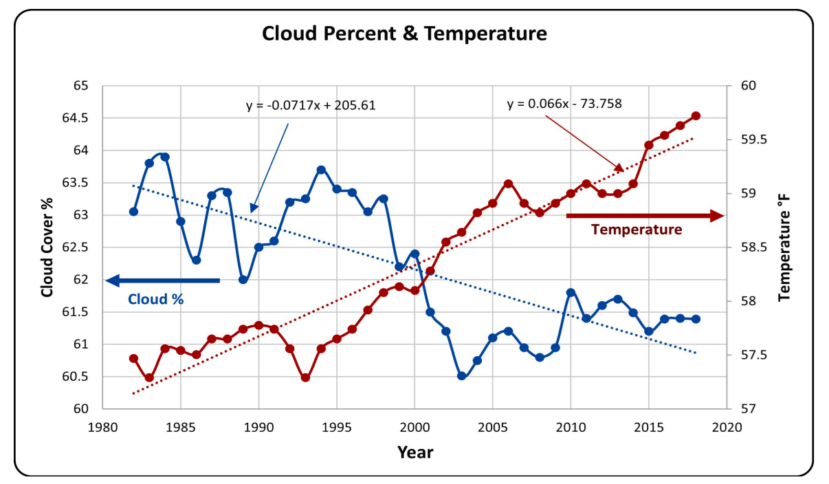
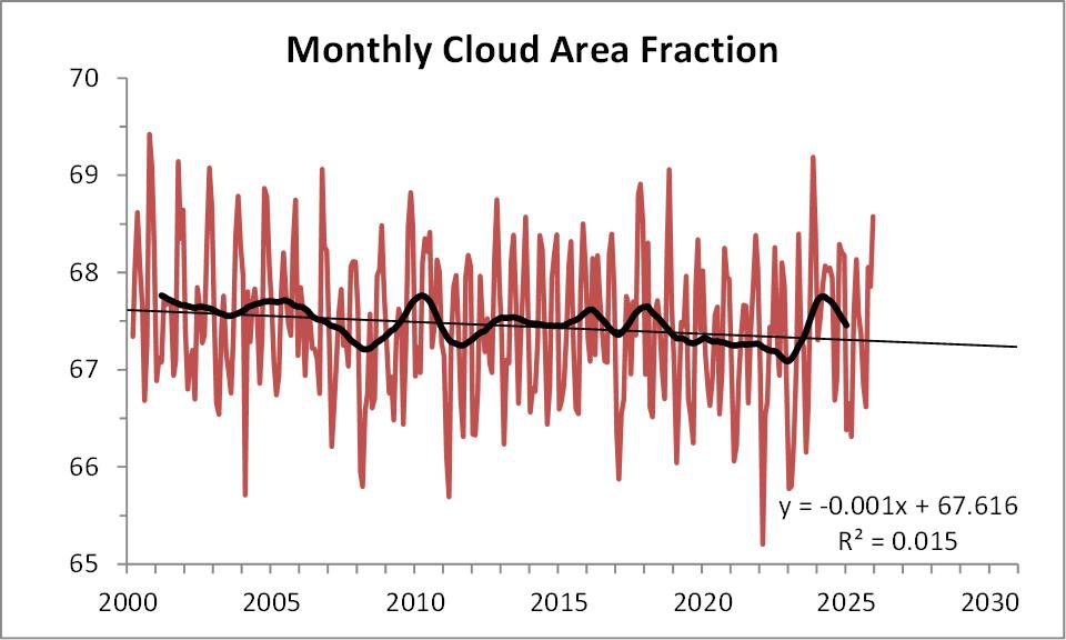
There is a consensus in the scientific community that the cloud fraction is the biggest uncertainty in climate change. The earth’s (about 60%) cloud fraction reflects about 50% of the sun rays. Prior to about 1980 little change in cloud fraction could be observed or measured it was assumed global cloud fraction was constant. Satellite data since about 1980 suggested that cloud fraction may be decreasing. A Cloud Reduction Global Warming, CRGW, theory (8) has been proposed to show how a natural sequence of related atmospheric processes can explain the cloud reduction and account for the observed increase in temperature, increase in specific humidity, and decrease in relative humidity.

From temperature and specific humidity, SH, the global annual Vapor Pressure Deficit, VPD(ga), can be calculated (8). VPD(ga) is a number that expresses how close the water concentration in the atmosphere is to the dew point, zero being the dew point (clouds highly probable) and the larger the number the less likely clouds will form somewhere on the earth.

Cloud fraction, CF(ga), measurement includes partly cloudy, high thin clouds, highly reflective rain clouds, and a lot of other cloud types with varying degrees of reflectivity. Enthalpy, En(ga) is a better indicator of non-reflectivity and is also correlates to CF(ga). VPD(ga) vs En(ga) does not have the baggage of CF(ga) and will be used in the model. Total enthalpy of the atmosphere has been shown to be equal to long wave radiation out (10) and at all altitudes including the surface data is proportional to long wave radiation out, see (10). Furthermore, ET(ga) is proportional to SH(ga), such that a change in ET(ga) = a change in SH(ga) and vs-vs.

Trenberth et al (2011) (12) documents total water evaporated/yr (Figure 9 in (12) ) from oceans, 413 (1000km^3/yr) and land at 73 (1000km^3/yr). The ocean data includes ice and clouds (62%) (both oceans and land). These measurements can be converted to ET(ga) per unit of earth’s surface area (1141(mm/yr/% of earth) for oceans and 494 (mm/yr/% of earth) for land), a 2.4 x higher ET rate from oceans. This difference in ocean vs land ET implies that any change in the earth’s land area, or percentage land under the sun’s zenith, or just land ET change may via CRGW theory change global temperature. This ocean vs land difference was observed in (18).

The Model

This is a first principles model not a statical model to show understanding of the proposed theory.

The model starts out with a reference year since ET(ga) and SH(ga) are proportional they need a real starting point (NOAA data between 1975 and 2024) . Next, a case study is chosen from any one or combination of: 1. change land size, 2. change axis shift of land under suns zenith, 3. change the ET of the land. Each case study calculates the ET(ga) (per year per unit area of earth’s surface) change from the ocean (and ice) and land ETs above (1141 and 494). Check the excel model attached for calculations. Table 1 gives some examples case from the model. Table 2 gives the input parameters and calculated ET(ga)s.

The model uses Clausius-Clapeyron derived Psychometric equations (see (8) for equations) and a sigmoidal graph of VPD(ga) vs Enthalpy, En(ga). The strategy of the model follows the path shown in Figure 1 and Figure 4. This path follows the adiabatic (constant En) line for increasing ET (SH) (to the left) or decreasing ET (SH) (to the right) to the point of SH(ga) change. Then follows the constant VPD(ga) line to the En(ga) predicted by Figure 2. (Follow VPD(ga) up for decreasing SH path, down for increasing SH path), see Figure 4 for a larger view of the path.

In Figure 2 the middle of the graph is NOAA data from (15) 1975 to 2024. The high and low asymptotes (all clouds and no clouds En(ga)) were calculated from Dubal (16) and Loeb (17) albedo data ratioed to known enthalpy data (adjusted for ocean and land area), all data at the same year. The parameters in the sigmoidal equation were then (by trial and error) fit to the data (20). Special attention was given to the sigmoidal fit matching the linear NOAA data. The sigmoidal graph allowed the model to work outside of the narrow NOAA range of VPDs.

Figure 1. Psychrometric chart showing the two-step process in the CRGW theory.

Figure 2. Sigmoidal fit of combined NOAA and CERES data.

The curious results of this model are that an initial decrease in earth’s ET(ga) will result in an increase ET(ga). This behavior can be seen on the psychrometric chart where the SH(ga) first decrease (for a -ET(ga)) on the adiabatic En line then increases on the constant VPD line per Figure 2. CRGW climate change is a two-step mathematical process where any time spent in the first step is only long enough to establish a new VPD to begin adjustment in cloud fraction. (Psychrometric charts are used by HVAC technicians to design air-conditioning systems, this is the first time constant VPD lines have been added to a Psychrometric chart to explain climate change, see Figure 4). The two-step process happens in yearly cycles leaving a trail of data on a diagonal with the two-step path from the starting point to the end point, if the change in ET is + or – or no change the observed data will be on the diagonal line, At either end of the sigmoidal graph this may change. At the end of the two-step path the resulting temperature and SH(ga must be solved by a convergence routine since the psychrometric equation contains mixed functions (log and linear). See attached model for equations.

The VPD(ga) vs cloud fraction is also a sigmoidal graph see Figure 3.

Figure 3. Sigmoidal graph of VPD vs Cloud Percent.

Figure 4. +/- ET(ga) change paths in the Model.

Other Model variables

Plumes occur over hot land and reach cloud level and can spread to cover areas larger than the surface they came from including the oceans. The hotter the more they spread. Plumes with low SH retard cloud formation (like a black parking lot). Plumes with high SH can make clouds (like a cooling tower). See (6) for more on plumes. The model uses plumes factors from 1x to 4x. Little research is done on global plumes other than we know they exist. The model shows plume factors can have a big effect on global temperature. The plume factors are set at 1x for size of land cases, and 2x for land under the sun’s zenith changes (for the expected hotter air), and 4x for special parcels where larger plumes are expected, see (6). The model applies the plume factor to the whole earth.

ET of special parcels like UHIs (urban heat Islands), land changes like forest to crop, or surface mining, see (8) for more on special parcels were estimated based on data from Mazrooei, et al (2021) (19). ET changes from +10 to -50 can be used.

Special parcel size is estimated at about 5 to 15% of the earth’s total land mass and growing, see (19) and (7) for more this.

Not in the model

Variations in the sun’s radiation to the earth. Easy to add just did not do it.

Volcanos also have historical climatic effects but appear to be short lived. Math like this essay may be applicable to volcanic effects on climate. Wet volcanoes (ones that have a lot of water in their plumes) cool the earth. Dry volcanoes (ones with just hot gas in the plumes) destroy clouds.

While CO2’s climatic effects are not discussed in this essay. CO2’s increase or decrease can be an indicator of changes in ET(ga) from vegetation. Decreasing CO2 indicates that vegetation is increasing the ET(ga) (more clouds, cooler), vs-vs. Current monitoring of CO2 concentration shows variation CO2 with the growing seasons.

Model results

The case studies in tables 1,2,3 show the earth’s temperature is very sensitive to axis rotation and land size. To the point that glaciers could be encouraged to grow or shrink with changes in the amount of land under the sun’s zenith (axis rotation), see (11), or change in the amount of land. Either one could be accented by vegetation changes.

The amount of increase in ET(ga) from cloud reduction seems to be related to the ratio of ET rate from oceans vs ET rate from land, for current data this ratio is 2-3 :1.

The historical coming and going of glaciers cloud be related to a series of cases like the following: Start at today’s conditions and rotate the earth so that less of the earth’s land is under the sun, (more clouds) the earth will cool. The earth’s vegetation will become more tropical near the sun’s zenith; (more clouds) the earth will cool more. Glaciers will grow, oceans will shrink, more land will appear, CO2 will decrease. Finaly enough land has appeared so that global ET increases (less clouds). The earth rotates back to more land under the sun’s zenith (less clouds). The earth becomes less tropical (less clouds) and the glaciers start to melt, seas rise and the earth returns to near current conditions.

Adding water to the atmosphere could return climate to 1975 conditions, but it is a lot of water.

Don’t worry about any of the cases, they will not happen in our time!

Discussion

Why wasn’t this theory already discovered (or has someone already proposed it and the author has not found it)? The answer could be simple: history could not see cloud change. The current climate change opened our eyes to the possible existence of this natural theory waiting to be discovered.

This expansion of the CRGW theory is intended to be a possible tool in the investigation of historical climate change to explore what did cloud fraction do as the earth changed over time and what future changes in the earth’s land mass might do to cloud fraction.

To the scientist that study earth’s changes over time: How well does this theory fit possible historic climate change vs earth’s land changes?

Thank You Anthony

For promoting diversity of thought

Bibliography

Author’s Papers

Bibliography continued

Atmospheric Moisture Transports from Ocean to Land and Global Energy Flows in Reanalyses (2011) by Kevin E. Trenberth, John T. Fasullo, and Jessica Mackaro web link Atmospheric Moisture Transports from Ocean to Land and Global Energy Flows in Reanalyses in: Journal of Climate Volume 24 Issue 18 (2011)
“HUMIDITY CONVERSION FORMULAS” by Vaisala Oyj (2013) web link Humidity_Conversion_Formulas_B210973EN-F (hatchability.com)
Climate Explorer web site Climate Explorer: Select a monthly field (knmi.nl) .
Physical Science Laboratory Monthly Mean Timeseries: NOAA Physical Sciences Laboratory
“Radiative Energy Flux Variation from 2001–2020” (2021) by Hans-Rolf Dübal and Fritz Vahrenholt web link: Atmosphere | Free Full-Text | Radiative Energy Flux Variation from 2001–2020 | HTML (mdpi.com)
Norman G. Loeb,Gregory C. Johnson,Tyler J. Thorsen,John M. Lyman,Fred G. Rose,Seiji Kato web link Satellite and Ocean Data Reveal Marked Increase in Earth’s Heating Rate – Loeb – 2021 – Geophysical Research Letters – Wiley Online Library
Figure 4 in 5 above and Met Office Climate Dashboard web Link Humidity | Climate Dashboard (metoffice.cloud)
. “Urbanization Impacts on Evapotranspiration Across Various Spatio-Temporal Scales” (2021) by Amir Mazrooei, Meredith Reitz, Dingbao Wang, A. Sankarasubramanian web link Urbanization Impacts on Evapotranspiration Across Various Spatio‐Temporal Scales – Mazrooei – 2021 – Earth’s Future – Wiley Online Library
StackOverlow Q and A scipy – Fit sigmoid function (“S” shape curve) to data using Python – Stack Overflow

5 3 votes

Article Rating

54 Comments

Inline Feedbacks

View all comments

strativarius

April 8, 2026 2:38 am

Why wasn’t this theory already discovered

In the first instance a religion smothers progress, it is about maintaining a status quo.
One example could be the thousand years of not much doing in the Christian world until the Renaissance in the late 1300s

My own humble guess is that a great many in science are now much like easily herded sheep.
They all need an income. Stephen Schneider let the cat out of the bag on [scientific] activism:

“…we have to offer up scary scenarios, make simplified, dramatic statements, and make little mention of any doubts we might have. This ‘double ethical bind’ we frequently find ourselves in cannot be solved by any formula. Each of us has to decide what is the right balance between being effective and being honest.” – Dr. Stephen Schneider, former IPCC Coordinating Lead Author, APS Online, Aug./Sep. 1996

And that’s precisely what we get. No new ideas on climate unless they happen to be Carbon dioxide related.

Bravo, sir.

gyan1

Reply to strativarius

April 8, 2026 10:50 am

“Why wasn’t this theory already discovered?”

This isn’t new. Many peer reviewed papers have concluded that cloud fraction is the dominant mechanism regulating Earth’s heat budget.

bnice2000

Reply to gyan1

April 8, 2026 1:43 pm

Certainly what has caused the slight warming since 1979 when these things started to be measured with satellites

MarkW

Reply to strativarius

April 8, 2026 1:27 pm

In your opinion, the collapse of the Roman Empire and the following dark ages had nothing to do with the lack of progress?
The lack of resources with which to pay people who did nothing but sit around and think had notihing to do with it?
It was all the fault of those pesky Christians and their unwillingness to upset the status quo?

wilpost

Reply to MarkW

April 8, 2026 2:23 pm

Pesky like DaVinci and Kepler and Galileo?

Ron Clutz

Reply to strativarius

April 11, 2026 9:20 am

Another study along the same lines is Decoupling CO2 from Climate Change— International Journal of Geosciences, 2024; Nelson & Nelson.

https://www.scirp.org/pdf/ijg_2024032514494686.pdf

Figure 10. This graph is the cloud fraction and is set forth on the left vertical axis. The temperature is on the right vertical axis and the horizontal axis represents the observation year. The information was extrapolated from figures prepared by Hans-Rolf Dubal and Fritz Vahrenholt [37].

Joseph Zorzin

April 8, 2026 3:13 am

off topic- sorry

‘OFFENSIVE to voters’: Mass Gov Healey decried for donut analogy on energy costs

Power the Future founder and executive director Daniel Turner discusses a social media video of Massachusetts Gov. Maura Healey using donuts to explain energy costs on ‘The Bottom Line.’

strativarius

Reply to Joseph Zorzin

April 8, 2026 4:39 am

When islands like Guam can capsize with more people on them and we get word salads like:

“So, Ukraine is a country in Europe. It exists next to another country called Russia. Russia is a bigger country. Russia is a powerful country. Russia decided to invade a smaller country called Ukraine. So, basically, that’s wrong, and it goes against everything that we stand for.” – K Harris

A doughnut explanation is hardly surprising.

wilpost

Reply to strativarius

April 8, 2026 2:27 pm

NATO Expanded to Russia’s Borders Just as if no Promise Were Made

NATO did expand to Russian borders, starting in 1999 to the present, for “defensive purposes”.
For many decades, M16 of the UK and CIA of the US have a common goal, aka “Europe’s security interests”, a euphonism to:

1) Weaken Russia (by using Ukraine as a proxy attack dog “for as long as it takes”),
2) Create internal unrest, by using Navalny, a political opponent of Putin.
3) Carve up Russia into 5 to 7 pieces; Russia would cease to exist.
4) Take control of Russia’s vast resources.
https://warontherocks.com/2019/11/promises-made-promises-broken-what-yeltsin-was-told-about-nato-in-1993-and-why-it-matters-2/.

The US/EU/UK has lots of experience extending influence, often by force

1) The US/EU/UK-instigated/financed, illegal coup d’etat in Kiev in 2014, violently ousted a Democratically elected President, and caused 116 dead, plus 184 with gunshot wounds, plus 760 with bodily injury
The Kiev coup was another violent attempt to further extend Western influence, often by force, to Russia’s borders, to enable the US/EU/UK to take over Ukraine and use it as a proxy-platform to “strategically weaken Russia, for as long as it takes”, according to US President Biden and his Secretary of Defense and Secretary of State.

2) A prior violent attempt caused Serbia to lose Kosovo, originally populated by Orthodox-Christion Serbs, who were displaced by Islamic Albanians., who rapidly increased their numbers by additional immigration and high rates of breeding.
Eventually, the Albanians totally over-whelmed the Serb population. Sarajevo was bombed by NATO until the Serbian Army withdrew from Kosovo. Kosovo had been part of Serbia for over 1000 years.

NOTE: If present trends continue, a similar displacement of the native populations of the UK, Germany, Spain and France, etc. will likely happen in a few decades.

Their angry, over-taxed, over-regulated native populations, already burdened by the wind/solar/batteries nonsense, and then further burdened by do-good bureaucrats and self-serving woke elites bringing in tens of millions of uninvited, unvetted, uneducated, unskilled, crime-prone, poor ghetto-trash, from dysfunctional Third-World countries.

Those folks are sucking from the multiple, government-program tits, while making 1) minimal efforts to produce goods and services, and 2) maximum efforts to be chaotic, culture-destroying burdens, the native populations never voted for. They would be a liability for the military defense of host countries.
In 2015, Trump closed the US borders to keep out undesirable folks from all over the world.

Denis

Reply to Joseph Zorzin

April 8, 2026 7:29 am

The Governor apparently thinks that the cost of a donut hole is the consequence of the cost of the wheat and other ingredients, omitting the cost of making it, packaging it, shipping it or the ingredients to the bakery and to the customer, taxes on each of the processes involved, the energy required to complete each step and other costs. Her argument is akin to those who think that the cost of our electricity is only the cost of generation, omitting everything required to deliver proper electricity to our wall outlets. She also seemingly thinks that electricity can be produced, stored and shipped in something as simple and cheap as a cardboard box. The woman has a startlingly ignorant knowledge of the process of making donuts, or electricity and probably everything else as does her staff who allow her to declare such ignorance. Nothing good can come from people like her wherever they work and only harm from those in positions of political power, and the harm is coming.

Joseph Zorzin

Reply to Denis

April 8, 2026 8:20 am

Very few people in Wokeachusetts dare to challenge her. One who is doing a great job is Mike Urban. He has a YouTube channel dedicated to slamming her every day. I’m surprised she hasn’t sent the state troopers after him. One of his recent videos spoofs Healey’s donut nonsense. It’s as follow:

This is Environmental Justice

Denis

Reply to Joseph Zorzin

April 8, 2026 9:56 am

Thanks.

Erik Magnuson

Reply to Denis

April 8, 2026 12:35 pm

Her argument is akin to those who think that the cost of our electricity is only the cost of generation, omitting everything required to deliver proper electricity to our wall outlets.

Unfortunately, only a minority of the population understands this fact. Back in the 1970’s, the invested capital in electric utilities was roughly 40% generation, 20% transmission and 40% distribution.

wilpost

Reply to Erik Magnuson

April 8, 2026 2:33 pm

HIGH COST/kWh OF W/S SYSTEMS FOISTED ONTO A BRAINWASHED PUBLIC
https://www.windtaskforce.org/profiles/blogs/high-cost-kwh-of-w-s-systems-foisted-onto-a-brainwashed-public-1
.
People are brainwashed to love wind and solar. They do not know by how much they screw themselves by voting for the elites who push them onto everyone.
.
If owned/controlled by European governments and companies, would be a serious disadvantage for the US regarding environmental impact, national security, economic competitiveness, and sovereignty
.
Western countries cajoling Third World countries into Wind/Solar and loaning them high-interest money to do so, will forever re-establish a neo-colonial-style bondage on those recently free countries.

What is generally not known, the more weather-dependent W/S systems, the less efficient the traditional generators, as they inefficiently (more CO2/kWh) counteract the increasingly larger ups and downs of W/S output. See URL
https://www.windtaskforce.org/profiles/blogs/fuel-and-co2-reductions-due-to-wind-energy-less-than-claimed
.
W/S systems add great cost to the overall delivery of electricity to users; the more W/S systems, the higher the cost/kWh, as proven by the UK and Germany, with the highest electricity rates in Europe, and near-zero, real-growth GDP.
.
At about 30% W/S, the entire system hits an increasingly thicker concrete wall, operationally and cost wise.
The UK and Germany are hitting the wall more hours each day.
The cost of electricity delivered to users increased with each additional W/S/B system
.
Nuclear, gas, coal and reservoir hydro plants are the only rational way forward.
Ignore CO2, because greater CO2 ppm in atmosphere is essential for: 1) increased green flora to increase fauna all over the world, and 2) increased crop yields to better feed 8 billion people.
.
Net-zero by 2050 to-reduce CO2 is a super-expensive suicide pact, to:
1) increase command/control by governments, and
2) enable the moneyed elites to become more powerful and richer, at the expense of all others, by using the foghorn of the government-subsidized/controlled Corporate Media to spread scare-mongering slogans and brainwash people, already for at least 40 years. Extremely biased CNN, MSNBC, NPR, PBS, NBC ABC, CBS come to mind.
.
Subsidies shift costs from project Owners to ratepayers, taxpayers, government debt:
1) Federal and state tax credits, up to 50% (Community tax credit 10%; Federal tax credit of 30%; State tax credit; other incentives up to 10%),
2) 5-y Accelerated Depreciation to write off of the entire project,
3) Loan interest deduction
.
Utilities forced to pay at least:
15 c/kWh, wholesale, after 50% subsidies, for electricity from fixed offshore wind systems
18 c/kWh, wholesale, after 50% subsidies, for electricity from floating offshore wind
.
Excluded costs, at a future 30% W/S annual penetration on the grid, based on UK and German experience:
– Onshore grid expansion/reinforcement to connect far-flung W/S systems, about 2 c/kWh
– A fleet of traditional power plants to quickly counteract W/S variable output, on a less than minute-by-minute basis, 24/7/365, which means more Btu/kWh, more CO2/kWh, more cost of about 2 c/kWh
– A fleet of traditional power plants to provide electricity during 1) low-wind periods, 2) high-wind periods, when rotors are locked in place, and 3) low solar periods during mornings, evenings, at night, snow/ice on panels, which means more Btu/kWh, more CO2/kWh, more cost of about 2 c/kWh
– Pay W/S system Owners for electricity they could have produced, if not curtailed, about 1 c/kWh
– Importing electricity at high prices, when W/S output is low, 1 c/kWh
– Exporting electricity at low prices, when W/S output is high, 1 c/kWh
– Disassembly on land and at sea, reprocessing and storing at hazardous waste sites, about 2 c/kWh
Total ADDER 2 + 2 + 2 + 1 + 1 + 1 + 2 = 11 c/kWh
.
Offshore wind full cost of electricity FCOE = 30 c/kWh + 11 c/kWh = 41 c/kWh, no subsidies
Offshore wind full cost of electricity FCOE = 15 c/kWh + 11 c/kWh = 26 c/kWh, 50% subsidies
The 11 c/kWh is for various measures required by wind; power plant-to-landfill cost basis.
This compares with 7 c/kWh + 3 c/kWh = 10 c/kWh from existing gas, coal, nuclear, large reservoir hydro plants.
Some of these values increase, due to inflation, and exponentially increase as more W/S systems are added to the grid.
.
The economic/financial insanity and environmental damage is off the charts.
Europe has near-zero, real-growth GDP. Its economy has been tied into knots by inane people.

Sparta Nova 4

Reply to Denis

April 8, 2026 12:47 pm

The cost of a donut HOLE is nada. The governor was talking about the donut (ring).

That silly nit aside, yes, correct.

DMacKenzie

Reply to Sparta Nova 4

April 9, 2026 7:21 am

But you can buy whole boxes of donut holes c/w sprinkles or glaze, so obviously the cost of them is easily determined….and “nada” ain’t correct…
/s

Sparta Nova 4

Reply to DMacKenzie

April 9, 2026 8:10 am

I based my comment on the image in the video. Donuts.

I went back just now and watched the video. Donut holes.

I recant my comment with apologies.

Yes. One can buy just donut holes, just as one can also buy just donuts.

Reminds me of a story from long ago. The older brother cut a deal with his younger brother. Mom had made donuts. Older offered younger all the donut holes and kept the donuts for himself. The donut holes given to the younger were just air “held” between 2 fingers. Mom got wind of it and made a batch of real donut holes for the younger, complete with frosting, sprinkles, etc. Obviously that story had nothing to do with anything on this page. It was a morality tale.

Cheers.

bnice2000

Reply to Joseph Zorzin

April 8, 2026 1:44 pm

One out of 25 “holes” was wind.. Bit of an over-estimate. !!

Most of them were FOSSIL FUELS.

Tom Abbott

April 8, 2026 3:27 am

You and RickWill should compare notes. You two might be describing some of the same effects.

Ben Vorlich

April 8, 2026 3:50 am

During the last peak glaciation
Surface Area Breakdown (Million km^2
)
Feature glaciation today
Land (Ice-Free) ~131 ~134
Land (Ice-Covered) ~44 ~22
Sea Ice (Ocean) ~45 ~22
Open Ocean ~290 ~340

How would this affect the model results?
Numbers from the internet

strativarius

Reply to Ben Vorlich

April 8, 2026 3:59 am

How would this affect the model results?

Doesn’t that depend on how one “tunes” the models?

Javier Vinós

April 8, 2026 5:13 am

This essay assumes wind is constant or its changes don’t affect evaporation. This is clearly not correct.

Bob Weber

April 8, 2026 6:27 am

Two nits: references 10-19 are not listed in the bibliography, and the three tables should have a white background for clearer reading using a browser with dark reader mode.

The author didn’t use his theory to explain specifically how CERES cloud fraction changed since 2000. What exactly changed over land to cause the global cloud reduction since 2000, and how can he be so sure this wasn’t mostly driven by the ocean?

Sparta Nova 4

Reply to Bob Weber

April 9, 2026 8:13 am

You are “violating” the single “control knob” feature of the earth energy systems. 🙂

How dare you! 🙂

ToldYouSo

Reply to Bob Weber

April 9, 2026 8:46 am

A liner curve fit with a slope of -0.1% and a degree of fit (R-squared) of only 0.015?

To me, looking at the range of variance in the data points comprising the red line line, the slope is insignificant AND one would need to perform a F-test of the data set to determine if the low R-squared value is statistically significant or not.

Denis

April 8, 2026 6:43 am

“On a global annual basis things calm down to not much change except climate change.” What do you mean by “climate change?” The only changes in climate supposedly caused by CO2 noted at present are small increases in temperature. There are no changes in hurricanes/typhoons, droughts, floods and so forth. Have you found climate changes other than temperature?

blais

Reply to Denis

April 9, 2026 9:35 am

The climate change in this paper is Global Annual which in our lifetime did not change much until about 1975. Change within a year is very chaotic and has a wind component which may average out over a year and therefore is not used in this paper. The paper theorizes what could have happened way before our lifetime.

Denis

April 8, 2026 6:56 am

“Start at today’s conditions and rotate the earth so that less of the earth’s land is under the sun, (more clouds) the earth will cool.”

If I understand correctly, you are saying that if the angle of the earth’s axis relative to the plane of the earth’s orbit is changed, that will alter the amount of sunlight striking land, which is mostly in the northern hemisphere, and thus alter the climate as well. Isn’t that one of the variables considered by the Milankovitch cycles?

Nicholas Schroeder

April 8, 2026 7:11 am

This is what “diverse” looks like.

Earth is cooler w atmos/watervapor/30% albedo not warmer.
Ubiquitous GHE balance graphics don’t + violate GAAP & LoT.
Kinetic heat transfer processes of contiguous atmos molecules render “extra” GHE energy upwelling from a BB surface impossible.
GHE = bogus & CAGW = scam.

-1

DMacKenzie

Reply to Nicholas Schroeder

April 8, 2026 4:40 pm

Well actually if the surface was say 15 C the outgoing radiation with no atmosphere would be about 390 watts by Planck equation, but the incoming sunlight would be 1360/4=340 less an albedo of about .13 like the Moon so about 295 watts…so Earth would on average be cooler without its atmosphere.

Again NS is so fun to troll…

Sparta Nova 4

Reply to DMacKenzie

April 9, 2026 8:51 am

You have it wrong. 1360/4 is only applicable on a narrow ring on a sphere based on northern/southern latitudes (~ 75.5 degree) and near the day-night terminators (~ 2 hr after dawn and before sunset at the nadir equator)..

The /4 only applies to a non-rotating flat earth.
The earth is not that simple model too often used.
The earth is not a perfect sphere, it is an oblate spheroid.
T^4 is temperature based.
Use of an average temperature over average surface area does not give a valid answer.

Tim Gorman

Reply to Sparta Nova 4

April 9, 2026 9:12 am

“Use of an average temperature over average surface area does not give a valid answer.”

Especially if you are using an arithmetic average instead of the average of an exponential curve.

DMacKenzie

Reply to Tim Gorman

April 10, 2026 4:35 pm

See point 5) foregoing

DMacKenzie

Reply to Sparta Nova 4

April 10, 2026 4:33 pm

you are so confused….area of a sphere is 4 times the area of its shadow…sunlight at our orbit is 1360 watts per sq.m times PI x R^2. It is distributed over a sphere of area 4x PI x R^2….
1) it is middle school simple. 2} the 4 x PI x R2 sphere IS rotating 3) Its a sphere for practical purposes, rounder than the average billiard ball. 4) obviously T^4 is temperature based
5) average temp, sure the real planet is a mosaic of different temperatures, each emitting at some factor x T^4, but average temp is accurate enough to show Shroeders “Earth is cooler not warmer with an atmosphere” is hogwash.

DMacKenzie

April 8, 2026 7:18 am

Fig 2 title… sigmoidal and atmosphere are mis-spelled…

Nicholas Schroeder

April 8, 2026 7:19 am

USCRN data clearly show RH & DB swapping BTU on a diurnal cycle acting as a thermal flywheel moderating the temperature swing.
This what differentiates Earth from Moon.

ToldYouSo

April 8, 2026 8:39 am

IMHO, the above article is an initial attempt to model the complex issue of Earth’s albedo dependence on global cloud fraction . . . a major climate factor not being analytically addressed to any significant degree in terms of considering “global warming” and its trending.

However, having said that, I was surprised to see the absence anywhere in the article of modeling the major effect of surface winds across both water and land areas as a determining factor in the local rates of EvapoTranspiration (ET).

The dependence of ET rate (correlatable to rate of energy exchange between liquid/land surfaces and the atmosphere) on surface winds largely falsifies this third sentence of the abstract as posted in the above article:
“Ocean’s global annual ET(ga) rate is relatively constant while land’s rate can change with local changes in EvapoTranspiration.”

The world’s oceans have significant variability in surface wind velocities over periods of years up to multiple decades due to variable frequency of events such as tropical storms/hurricanes/typhoons, the PDO (El Niño/La Niña events), the AMO/AMOC, and solar heating variability that effects the near-surface velocities in the Hadley, Ferrel and Polar major circulation cells in the Earth’s NH and SH.

See the 2024 AGU publication “Recent Decline in Global Ocean Evaporation Due To Wind
Stilling”, Ning Ma et.al. (https://agupubs.onlinelibrary.wiley.com/doi/pdf/10.1029/2024GL114256 )

Also, the online water surface evaporation calculator (https://www.omnicalculator.com/physics/evaporation-rate ) shows the following calculated variation for an assumed constant air temperature of 70 deg-F and assumed constant air RH of 50%:
— for cross-surface air velocity = 1 mph, evaporation flux rate = 0.05 lbm/sec/ft^2
— for cross-surface air velocity = 30 mph, evaporation flux rate = 0.45 lbm/sec/ft^2
— for cross-surface air velocity = 60 mph, evaporation flux rate = 0.85 lbm/sec/ft^2
So the effect of wind on evaporation from a water surface is substantial, up to a factor of 10 or more for natural variability of wind speeds across oceans, and this is not even considering the additional evaporation rate that would be caused by waves “breaking” on the water’s surface.

Nicholas Schroeder

Reply to ToldYouSo

April 8, 2026 2:04 pm

There is no consensus on a numerical value for the albedo.

ToldYouSo

Reply to Nicholas Schroeder

April 8, 2026 6:17 pm

Yes, simply because there is no “consensus” method for scientifically predicting future areal cloud coverage on Earth based on current weather/climate parameters.

Nevertheless, a rough average albedo value of around 0.30 has been used historically (and assumed to be more or less constant) based on ground and satellite measurements/calculations of Earth’s radiation energy balance.

Sparta Nova 4

Reply to ToldYouSo

April 9, 2026 8:53 am

Go outside.
Take off your shoes.
Put one foot on the blacktop driveway and the other on the lawn grass.
Tell me those can be averaged.

ToldYouSo

Reply to Sparta Nova 4

April 9, 2026 11:14 am

“Put one foot on the blacktop driveway and the other on the lawn grass.
Tell me those can be averaged.”

Hah! . . . you have made the classic, sophomoric mistake of confusing temperature with radiation energy. Albedo is a measurement of absorbed versus reflected radiant energy; on the other hand temperature (which can be sensed by one’s skin/feet, although not all that accurately) is an intrinsic, aka “intensive”, physical of parameter of matter representing the average kinetic energy of atoms and molecules within a substance, indicating its hotness or coldness.

And to be clear, yes, one gallon of water at, say, 100 deg-F temperature can be mathematically averaged with a separate gallon of water at, say, 60 deg-F temperature to accurately predict mixing the two in a two-gallon or larger container will yield an average water temperature of—don’t ya know—80 deg-F.

Tim Gorman

Reply to ToldYouSo

April 10, 2026 3:55 am

“And to be clear, yes, one gallon of water at, say, 100 deg-F temperature can be mathematically averaged with a separate gallon of water at, say, 60 deg-F temperature to accurately predict mixing the two in a two-gallon or larger container will yield an average water temperature of—don’t ya know—80 deg-F.”

This is also a classic sophomoric mistake of confusing two objects with one. When you mix the two separate containers of water you are creating a separate, single container. First off, the “water” in each container have to be exactly the same in order to reach the “average” temperature, any difference in them (e.g. salinity) will result in a different final temperature. This is similar to the climate science garbage of assuming you can take two parcels of the atmosphere and calculate an average temperature when the two parcels of air have totally different makeups – different humidity, different pressures, and different components (e.g. CO2 density).

“can be mathematically averaged” are the applicable words. Statisticians think you can average anything with no need for the components having a physical reality. E.g. you can average the heights of Arabian stallions with the heights of Shetland ponies and get an average height for “horses”. To a statistician it doesn’t matter that you are averaging two physically totally different things. Like averaging the temperature on Pikes Peak with the temperature in Colorado Springs to get an “average” temperature.

ToldYouSo

Reply to Tim Gorman

April 10, 2026 8:28 am

“This is also a classic sophomoric mistake of confusing two objects with one.”

So says you. However, most people with an IQ above room temperature (pardon the pun) would recognize that one gallon of water at 100 deg-F is distinctly different from one gallon of water at 60 deg-F, referring to one as relatively “warm” and the other as relatively “cool”.

ToldYouSo

Reply to ToldYouSo

April 8, 2026 6:08 pm

Ooop . . . my mistake: I just noticed that the flux rates I posted above should all have been in units of lbm/hr/ft^2 . . . no way those could be in units of lbm/sec/ft^2! The referenced online calculator is clear about the units and I just botched the copy & pasting of such. However, the ratio-ing of fluxes with wind speed is correct.

Mea culpa!

DMacKenzie

Reply to ToldYouSo

April 9, 2026 7:41 am

You chose 50% RH….most of the weather stations I look at vary around a mean of 75 to 80%, Didn’t run the Omni calculator to see the 1 to 30 mph evaporative flux change…

ToldYouSo

Reply to DMacKenzie

April 9, 2026 8:21 am

Here, for your convenience, from the online water surface evaporation calculator (https://www.omnicalculator.com/physics/evaporation-rate ) for an assumed constant air temperature of 70 deg-F and assumed constant air RH of 75%:
— for cross-surface air velocity = 1 mph, evaporation flux rate = 0.03 lbm/hr/ft^2
— for cross-surface air velocity = 30 mph, evaporation flux rate = 0.22 lbm/hr/ft^2
— for cross-surface air velocity = 60 mph, evaporation flux rate = 0.43 lbm/hr/ft^2

Still, even at 75% RH, more than an order of magnitude difference in wind-driven evaporation rates between 1 mph and 60 mph wind speeds, easily within the range of variability in natural winds.

DMacKenzie

Reply to ToldYouSo

April 10, 2026 5:44 pm

I roughly worked out your .03 at 1 mph and .22 at 30 mph and that’s cooling of about 90 watts/sq.m increasing to 650 watts/sq.m from calm to windy conditions…

ToldYouSo

Reply to DMacKenzie

April 11, 2026 8:03 am

I didn’t double check your calculations, but trust them. The latent heat of evaporation of water is HUGE compared to other weather effects such as convective cooling by winds, or the latent heat of ice<–>liquid water phase change, or even a 10% swing in Earth’s surface albedo (about 341 W/m^2 * 0.7 *0.1 = 24 W/m^2).

So, just consider your range of 90–650 W/m^2 from ET-over-water as varies by natural winds against the assertions by Trenberth et.al. that Earth’s energy flux imbalance can be calculated as an accurate value of 0.6 W/m^2. Good grief!

Neo Conscious

April 8, 2026 8:48 am

The interactions between temperature, clouds and other atmospheric phenomena (and thus climate) are very complex and go beyond reflective effects. One cloud phenomenon with a huge impact is storms and the massive heat transfer they facilitate, similar to mechanized condenser cooling systems. Storms are the most intense cloud phenomena, and they provide the most complex weather variables.

The large heat transfer associated with phase changes initially leads to surface cooling during evaporation. The latent heat is released in distant locations where it is more likely to escape directly into space, whether at higher elevations or latitudes. This precipitation effect accounts for the highest percentage of the meridional heat transfer away from equatorial regions. The heat released during storms generates increased convection which leads to increased precipitation and heat release.

While cloud fraction is a huge variable in climate, other variables that specifically impact storm formation such as atmospheric particulates also have significant impacts.

Jimmie Dollard

Reply to Neo Conscious

April 8, 2026 9:39 am

Wind is also the primary factor in wild fires. Low wind-we control wild fires. High winds- we can’t control and they get big. The other things hardly matter.

Neo Conscious

Reply to Jimmie Dollard

April 8, 2026 5:37 pm

Yes, and the wind variable is also huge in accelerating evaporation rates and meridional heat transfer.

Alan

April 8, 2026 9:55 am

I’m surprised no one has noticed that as the number and size of telescopes owned by ameatur astronomers increase, there is a proportional increase in clouds. Now put that in your computer models.