From Dr. Roy Spencer’s Global Warming Blog
by Roy W. Spencer, Ph. D.
The Version 6.1 global average lower tropospheric temperature (LT) anomaly for September, 2025 was +0.53 deg. C departure from the 1991-2020 mean, up from the August, 2025 anomaly of +0.39 deg. C.
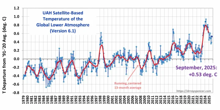
The Version 6.1 global area-averaged linear temperature trend (January 1979 through September 2025) remains at +0.16 deg/ C/decade (+0.22 C/decade over land, +0.13 C/decade over oceans).
The following table lists various regional Version 6.1 LT departures from the 30-year (1991-2020) average for the last 21 months (record highs are in red).
| YEAR | MO | GLOBE | NHEM. | SHEM. | TROPIC | USA48 | ARCTIC | AUST |
| 2024 | Jan | +0.80 | +1.02 | +0.58 | +1.20 | -0.19 | +0.40 | +1.12 |
| 2024 | Feb | +0.88 | +0.95 | +0.81 | +1.17 | +1.31 | +0.86 | +1.16 |
| 2024 | Mar | +0.88 | +0.96 | +0.80 | +1.26 | +0.22 | +1.05 | +1.34 |
| 2024 | Apr | +0.94 | +1.12 | +0.76 | +1.15 | +0.86 | +0.88 | +0.54 |
| 2024 | May | +0.78 | +0.77 | +0.78 | +1.20 | +0.05 | +0.20 | +0.53 |
| 2024 | June | +0.69 | +0.78 | +0.60 | +0.85 | +1.37 | +0.64 | +0.91 |
| 2024 | July | +0.74 | +0.86 | +0.61 | +0.97 | +0.44 | +0.56 | -0.07 |
| 2024 | Aug | +0.76 | +0.82 | +0.69 | +0.74 | +0.40 | +0.88 | +1.75 |
| 2024 | Sep | +0.81 | +1.04 | +0.58 | +0.82 | +1.31 | +1.48 | +0.98 |
| 2024 | Oct | +0.75 | +0.89 | +0.60 | +0.63 | +1.90 | +0.81 | +1.09 |
| 2024 | Nov | +0.64 | +0.87 | +0.41 | +0.53 | +1.12 | +0.79 | +1.00 |
| 2024 | Dec | +0.62 | +0.76 | +0.48 | +0.52 | +1.42 | +1.12 | +1.54 |
| 2025 | Jan | +0.45 | +0.70 | +0.21 | +0.24 | -1.06 | +0.74 | +0.48 |
| 2025 | Feb | +0.50 | +0.55 | +0.45 | +0.26 | +1.04 | +2.10 | +0.87 |
| 2025 | Mar | +0.57 | +0.74 | +0.41 | +0.40 | +1.24 | +1.23 | +1.20 |
| 2025 | Apr | +0.61 | +0.77 | +0.46 | +0.37 | +0.82 | +0.85 | +1.21 |
| 2025 | May | +0.50 | +0.45 | +0.55 | +0.30 | +0.15 | +0.75 | +0.99 |
| 2025 | June | +0.48 | +0.48 | +0.47 | +0.30 | +0.81 | +0.05 | +0.39 |
| 2025 | July | +0.36 | +0.49 | +0.23 | +0.45 | +0.32 | +0.40 | +0.53 |
| 2025 | Aug | +0.39 | +0.39 | +0.39 | +0.16 | -0.06 | +0.69 | +0.11 |
| 2025 | Sep | +0.53 | +0.56 | +0.49 | +0.35 | +0.38 | +0.77 | +0.32 |
The full UAH Global Temperature Report, along with the LT global gridpoint anomaly image for September, 2025, and a more detailed analysis by John Christy, should be available within the next several days here.
The monthly anomalies for various regions for the four deep layers we monitor from satellites will be available in the next several days at the following locations:
The new Monckton Pause extends to 30 months starting in 2023/04. The average of this pause is 0.62 C. The previous Monckton Pause started in 2014/06 and lasted 107 months and had an average of 0.21 C. That makes this pause 0.41 C higher than the previous one.
+0.156 ± 0.040 C.decade-1 k=2 is the trend from 1979/01 to 2025/09.
+0.027 ± 0.010 C.decade-2 k=2 is the acceleration of the trend.
My prediction for 2025 from the 2025/03 update was 0.43 ± 0.16 C k=2.
My prediction for 2025 from the 2025/04 update was 0.47 ± 0.14 C k=2.
My prediction for 2025 from the 2025/05 update was 0.46 ± 0.11 C k=2.
My prediction for 2025 from the 2025/06 update was 0.47 ± 0.10 C k=2.
My prediction for 2025 from the 2025/07 update was 0.46 ± 0.08 C k=2.
My prediction for 2025 from the 2025/08 update was 0.46 ± 0.06 C k=2.
My prediction for 2025 from the 2025/09 update is 0.48 ± 0.05 C k=2.
You should be looking at the absorbed solar radiation..
….. but that would give the game away, wouldn’t it !.
Are temperatures actually measured to +/- 0.01 deg C? How are the sensors calibrated? Why are peaks in the doublets separated by 3 years?
The only thermometers in the field that can measure to this accuracy are the Argos buoys. A quick search did not reveal whether they use a platinum resistance thermometer (PRT) or a thermistor. I worked in a chemical research lab and we had a primary reference quality platinum resistance thermometer that we used to calibrate the working PRTs. It was designed and calibrated to be accurate to ±0.001 K from liquid nitrogen to ±0.010 K at the melting point of zinc. The thermometer itself was several thousand dollars, the calibration was even more, and the ohm meter to read it was even more. It was very delicate and not used for anything except calibrating the less expensive PRTs. The primary reference would normally go back to the cal lab annually. This is equipment and expense way above the typical weather station. I don’t think the weather stations get calibrated often enough either.
Not even the Argo floats are that accurate. The float accuracy is the sum of every component in the float, not just the sensor alone. Float uncertainty is around .3C to .5C at best.
Surely you’re not questioning the PROBITY of temperatures reportage, Tim?
(and we haven’t even touched on the PROVENANCE or the PRESENTATION of the temperatures reportage yet).
Agree with what Tim Gorman wrote. Geoff S
Sounds like temperature probes’ results need to establish some form of Method Detection Limit (MDL).
https://www.epa.gov/cwa-methods/method-detection-limit-frequent-questions
MDL is basically arrived at by knowing the resolution of a given instrument. Anything below that resolution limit is fundamentally unknown regardless of what statistical tools are used to derive a mean value.
If you look at a probability distribution the values on the distribution will be at the resolution limit, i.e. ±0.5 of the last known digit. Calculation cannot change that LIMIT, only instruments with higher resolution.
Tim, I think that you meant to say “that precise.” Accuracy is a whole different ball game.
UAH only uses PRTs to measure the hot calibration target. The global average temperature measurement is computed via a complex model using inputs that are themselves computed from yet more upstream models that process the O2 emissions. [Christ et al. 2003] say the spot measurements have an uncertainty on the order of 1 C, but through the averaging process these gets reduced to about 0.2 C at the global level. There is only 1/5th scaling here despite there being 9504 spot measurements because the degrees of freedom on the grid is only 26.
(…)but through the averaging process these gets reduced(…) Hmm, so I measure your blood cholesterol, and the blood cholesterol of the rest of your village, the village average will somehow reduce the uncertainty of your blood cholesterol measurement?
Well said. The climate brigands still don’t understand when the rule of large samples can be used..
.. and when it can’t. !!
They don’t even understand what sample size is! Single measurements of different things don’t create a large sample size. It creates a large number of samples of size 1. Thus when you try to calculate the standard deviation of the sample means it becomes the standard deviation of the concatenated samples.
SEM = SD/sqrt[n] –> SEM = SD
since sqrt[1] = 1
“They don’t even understand what sample size is!”
https://www.statology.org/understanding-sample-size/
“Single measurements of different things don’t create a large sample size.”
Wrong.
From your reference.
This code returns Required sample size: 34.0, indicating that for a t-test with these parameters, you’d need at least 34 observations in each group to detect a medium-sized effect with 80% statistical power.
“in each group” means multiple samples each of size 34.
It’s describing a t-test. You are comparing two groups to see if there is a difference between the population means. You take a single sample from each group.
Really, just try to understand, rather than trying to find loop holes.
Each group would need 34 members in it. Two groups is multiple isn’t it? The point is that a single sample can’t be used to determine anything about a population.
You miss the entire purpose of the page YOU referenced. It isn’t to show that a single sample can be used to determine anything about a population’s parameters with any accuracy.
Are you going to insist that a single sample and the statistics from that sample can provide accurate statistical parameters for a population?
“Each group would need 34 members in it. Two groups is multiple isn’t it?”
Sigh – yes there are two samples. You are performing a 2-sample t-test. The clue is in the name. This has nothing to do with the incorrect claim that “Single measurements of different things don’t create a large sample size.”
Please stop trying to drag me into another one of your inane argument spirals. You’ve been spouting this nonsense for years and refuse to even consider you might be the one who doesn’t understand this.
Sample size means the size of the sample – it’s as simple as that.
“You miss the entire purpose of the page YOU referenced.”
I “referenced” it as it was the first thing that came up when I searched for sample size. If it’s making the claim you say it is then you need to quote it, and I’ll explain why it’s wrong. But for starters
How does that square with your claim that
“It isn’t to show that a single sample can be used to determine anything about a population’s parameters with any accuracy.”
“Are you going to insist that a single sample and the statistics from that sample can provide accurate statistical parameters for a population?”
Yes. A random independent sample can provide accurate information about the population. How accurate depends on the size of the sample compared with the variance, and assuming you are capable of measuring the things accurately. That’s what people who understand this have been saying for the last century or so.
“Sample size means the size of the sample – it’s as simple as that.”
It means a SAMPLE of the same thing. As per the start of this sub-thread you can’t take a measurement of cholesterol from one person and a measurement of blood pressure from a different person, concatenate them into a single data set and say you have created a sample of size 2.
Similarly you can’t take a measurement of temperature from Las Vegas and a measurement of temperature from Miami, concatenate them into a single data set, and then say you have one temperature sample with a size of two. What you actually have is two temperature samples of size one. Therefore the SEM becomes the SD of the two data points since the sqrt[1] = 1.
It’s like measuring the bore size of a 350cu Chevy, a 426 Chrysler hemi, and a 40hp/4cylinder Farmall tractor engine and saying you have a sample size of 3. And then saying the accuracy of the average bore size is the SD of the three measurements divided by sqrt[3]. SD/sqrt[3] is *NOT* the accuracy of the average, it is how precisely you have located the average value – two entirely different things. You actually have three samples of size one – so again the SEM is the SD of the values.
You are, once again, exhibiting the meme of a blackboard statistician that thinks “numbers is just numbers”.
“ A random independent sample can provide accurate information about the population”
No, it can’t, not if the sample is of reasonable size. The clue is that you have to ASSUME that the SD of the single sample is the same as the SD of the population in order to calculate an SEM. You have no good way to tell if the sample SD is the same as the population SD, you just have to ASSUME that it is. The kicker is that if the SD of the sample *IS* the same as the SD of the population then the SEM is probably useless since it’s highly unlikely that a sample that has a different mean than the population will have the exact same SD as the population.
The clue here is that the SEM is defined as the standard deviation of a set of sample MEANS, “means” as in plural. If you only have one sample then you are only ESTIMATING what the actual SEM is. Estimating a value actually ADDS to the measurement uncertainty, i.e. increases the SEM. How much it increases it is the big question.
None of this actually changes what the SEM is – a metric for how precisely you have located the population mean. It is *NOT* the accuracy of the population mean. Even with VERY LARGE systematic measurement uncertainty the SEM can be made very small by using large sample sizes.
This is the big problem with climate science. Climate science assumes that a small SEM implies an accurate mean value. It doesn’t imply that at all. It requires the application of your typical meme of “all measurement uncertainty is random, Gaussian, and cancels”.
“It means a SAMPLE of the same thing.”
You really need to explain what you mean by “the same thing”.
“you can’t take a measurement of cholesterol from one person and a measurement of blood pressure from a different person, concatenate them into a single data set and say you have created a sample of size 2. ”
Well – duh. You want to be measuring the same attribute.
“Similarly you can’t take a measurement of temperature from Las Vegas and a measurement of temperature from Miami”
Temperature is the same thing. You can average two temperatures, you cannot average cholesterol and blood pressure. As I said you need to define what you mean by “same thing”.
Not that this is how you would do it, but it’s entirely possible to estimate the average temperature of the earth, where the average temperature is the mean of the population and the population is the entire earth’s surface, by taking the temperature of two entirely random locations on the earth. It would give you a pretty rotten estimate given it’s a sample of size 2. You would get a better estimate by taking a larger sample.
“Therefore the SEM becomes the SD of the two data points since the sqrt[1] = 1.”
No. That would be the SEM if you only had a single measurement, i.e. a sample of size 1. Naturally in that case the sampling distribution is identical to the population distribution.
Rest of your rant ignored for now.
Let’s get more specific. Exactly what is the population of temperatures that you are talking about?
Are the “samples” of that population repeatable measurements of the property that is being determined?
Does the experimental standard deviation of the mean derived from those measurements of a property provide a measure of the dispersion of the measurements that are attributable to the mean?
Does the experimental standard deviation of the mean describe the likelihood of observing different outcomes in a random process, that is, the probability of measuring a given value in the next measurement?
Here is an excerpt from NBS Special Publication 747, Statistical Concepts in Metrology- With a Postscript on Statistical Graphics
Using metrology references, show how the references justify using the experimental standard deviation of the mean to describe the dispersion of measurements surrounding the limiting mean.
There is one and only one way that can occur. Let’s see if you can explain what it is and when it is used to describe measurement uncertainty.
“Exactly what is the population of temperatures that you are talking about?”
I wasn’t talking specifically about temperatures, just what sample size means. If you are talking about temperatures, then the population is whatever you are trying to get a sample of. Let’s assume you are talking about global temperature, than the population is the surface of the earth, or for UAH the lower troposphere. It may also be for a specific point in time or over a longer time span.
But as I keep trying to explain, you don’t actually do this using a random sample. That would be far to difficult. So you are relying on reading at fixed, non-random points, or a systematic sample over the entire earth.
“Are the “samples” of that population repeatable measurements of the property that is being determined?”
What samples? I don’t see how sampling can be repeatable in the sense you mean it, given the sample is random.
“Does the experimental standard deviation of the mean derived from those measurements…”
What “experimental standard deviation of the mean”. That’s the term the GUM uses when you are measuring the same thing repeatedly. It uses exactly the same maths as a statistical sample, becasue the laws of probability are the same.
“measurements of a property provide a measure of the dispersion of the measurements that are attributable to the mean?”
Yes – that’s a roundabout way of describing the SEM.
“Does the experimental standard deviation of the mean describe the likelihood of observing different outcomes in a random process”
Again, that’s what the SEM is – the standard deviation of the sampling distribution.
“…that is, the probability of measuring a given value in the next measurement?”
In theory yes. But it depends on what you mean by the next measurement. E.g. the SEM of the global anomaly for 2024 does not predict what the anomaly will be in 2025 – because the global temperatures may have changed. What it does give you is a way of determining if any difference is statistically significant.
“Here is an excerpt”
which just describes what a standard deviation is. Why do you keep doing this?
“Using metrology references, show how the references justify using the experimental standard deviation of the mean to describe the dispersion of measurements surrounding the limiting mean”
The standard error of the mean does not describe the dispersion of measurements around the mean. That would be the standard deviation.
It has to be “repeatable” in the sense that you are measuring the same thing. That is, the temperature of an air parcel.
Mr. Bellman: Yeah, “trying to find loopholes” is no way to gain a better understanding of your theory. I observe that you never try to gain a better understanding of your theory.
“t represents how many units from a population”
““Single measurements of different things don’t create a large sample size.””
bellman: “Wrong.”
Nope. Not wrong. Single measurements of different things are *NOT* units from the same population. Single measurements of different things are single samples of many different populations.
You have *still* not figured out that you can’t take a corral full of a mix of Shetland ponies and quarter-horses and say that single measurements of each form a sample of a “population”. The values at best will form a multi-modal distribution in which standard deviation is useless as a statistical descriptor. It’s no different than mixing single measurements of temperature in the NH and SH together – you wind up with a multi-modal distribution in which the SD is useless. If the SD is useless then the SEM is useless as well since it is derived from the SD.
Single measurements of different things under different environmental conditions will *NOT* produce a Gaussian distribution of random values that can be assumed to cancel. If they don’t cancel then the SEM can’t be used as the measurement uncertainty either. And it is the SEM that gets divided by sample size, not the measurement uncertainty.
Single values of different things represent a sample size of 1. That single measurement is the total population for that “different thing”.
“Nope. Not wrong.”
Yep. Very wrong.
“Single measurements of different things are *NOT* units from the same population.”
Do you really think a population has to have identical things? Take the population of the US. Are they all the same person?
“Shetland ponies and quarter-horses”
And we are back to your horse fetish. Please try to make a sensible argument rather than just repeating the same nonsense every time. You need to define your population. Why do you want to combine just two breads of horses. You can do it, but you have to ask yourself what do you want to find out.
“It’s no different than mixing single measurements of temperature in the NH and SH together – you wind up with a multi-modal distribution in which the SD is useless.”
Produce some evidence. Then explain why that matters more than say the difference between land and ocean, or the tropics and the poles. Of course you can look at different regions separately. But you can still treaty the globe as a single population.
Here’s the distribution UAH gridded data separated by North and South (not area weighted).
And here they are combined. Can you spot the different modes?
“If the SD is useless then the SEM is useless as well since it is derived from the SD.”
Why do you think the SD is useless? In the case of your 2 modal mix it will be a good indication of how far apart the two population means are.
“Single measurements of different things under different environmental conditions will *NOT* produce a Gaussian distribution of random values that can be assumed to cancel.”
How many more times do I have to explain that the distribution does not have to be Gaussian. The SEM = SD / √N is true regardless of the distribution, and CLT shows that an IID sample will have a sampling distribution that tends to a Gaussian regardless of the population distribution. This is very fundamental stuff.
That is true. However, you leave out some very pertinent assumption. The SEM is only a statistic that describes how well the mean (average) of the sample means distribution (multiple samples) estimates the population mean. It does not describe the population statistical parameter of the dispersion of the data around that mean, i.e. the standard deviation.
In fact, the common equation of SEM = σ/√n that when rearranged is σ = SEM * √n realistically describes the population standard deviation only if the population distribution is normal. It does not work if the population distribution is skewed, which requires an asymmetric measurement uncertainty interval to describe the dispersion of actual measurements.
From the GUM.
Read these carefully. Why would one EVER need an asymmetric uncertainty interval if the SEM always gives a normal distribution per the CLT? Is it possible that the GUM is describing the need for an asymmetric uncertainty interval due to the dispersion of measurements around the mean?
“The SEM is only a statistic that describes how well the mean (average) of the sample means distribution (multiple samples) estimates the population mean.”
Gibberish. Really, how difficult would it be for you to just find a simple text describing what the SEM is and understand it. The SEM is a description of the sampling distribution. It describes how close any one sample of a specified size is likely be to the population mean. It is not describing the mean of multiple samples.
It is talking about the mean of an individual sample, not as you are implying the mean of the means of multiple samples.
“In fact, the common equation of SEM = σ/√n that when rearranged is σ = SEM * √n realistically describes the population standard deviation only if the population distribution is normal.”
You’re contradicting yourself. SEM = σ/√n does not depend on the population being normal. So σ = SEM * √n dos not either. If, for some strange reason you wanted to estimate the population standard deviation from the SEM, it’s still just as correct regardless of the shape of the population.
What you possibly mean to say is that standard deviation does not fully describe the distribution unless it’s normal. And that’s why the CLT is useful.
“ It does not work if the population distribution is skewed, ”
You are still missing the point. SEM is describing the sampling distribution, it is describing the shape of the population.
“Read these carefully.”
Why? You keep posting endless copies of text with no context, and claim I should be able to misinterpret the same way as you do. Explain what you think it says, and then we can have a discussion about whether it does or not.
“Why would one EVER need an asymmetric uncertainty interval if the SEM always gives a normal distribution per the CLT?”
Well, for one thing the CLT does not “always give a normal distribution”. What is says is the sampling distribution will tend towards a normal distribution as sample size increases. How quickly this happens will depend on the shape of the distribution in the first case. A small sample of a highly skewed population will still be skewed.
Another reason would be if you are deriving measurements using a non linear function.
“It describes how close any one sample of a specified size is likely be to the population mean. It is not describing the mean of multiple samples.”
The concept of the SEM is built upon the central limit theorem. The CLT theorem holds that the means of multiple samples, when combined into a data set, will tend to a Gaussian distribution. The mean of that Gaussian distribution will thus be the best estimate of population mean and how precise that estimate will be is determined by the size of the samples.
A single mean from a single sample can *NOT* generate a Gaussian distribution of sample means. Therefore the CLT doesn’t apply. That means that an SEM GUESSED at by using the SD of the single sample as the population SD has a huge uncertainty of its own built in because you simply can not know how closely the SD of the single sample represents the population SD. If you *do* know the difference between the actual population SD and the sample SD then the SEM becomes useless because knowing the SD of the population means you also know the average of the population.
If the SEM obtained from a single sample has a in-built uncertainty then how can it accurately represent the uncertainty of the average? What factor do you use to add to the SEM to represent its own in-built uncertainty?
“The concept of the SEM is built upon the central limit theorem.”
I don’t think it is. I couldn’t tell you the history, but it’s possible to derive the SEM equation entirely from probability theory. It’s a simple application of the fact that variances add.
“The CLT theorem holds that the means of multiple samples, when combined into a data set”
It holds that the mean of set of IID random variables will be a random variable that tends to a Gaussian distribution. What you describe is a consequence of that,
“A single mean from a single sample can *NOT* generate a Gaussian distribution of sample means.”
You don;t need to generate the distribution. You estimate that through the magic of mathematics.
“Therefore the CLT doesn’t apply.”
It very much does. It allows you to assume that given a large enough sample the sampling distribution will be close to Gaussian.
If you did what you keep suggesting, and estimate the distribution experimentally, there would be no need to apply the CLT. You would be able to see how close you were to a Gaussian.
“That means that an SEM GUESSED at by using the SD of the single sample as the population SD has a huge uncertainty of its own built in”
Thanks for highlighting the dumbest part of your comment. The population standard deviation is usually estimated from the sample SD, but that hardly amounts to “guessing”. Bu that logic every measurement you make of one of your lumps of wood is just a guess.
Now of course you are right that there is some added uncertainty if you only have a small sample size – that’s why you use a student distribution rather than a Gaussian. Or you can use methods that directly estimate the uncertainty of the standard deviation.
But none of this has anything to do with your claim that you have to use multiple samples. That factor you never take into account is that multiple samples just mean more sampling. If you take 20 samples of size 20, you have to make 400 measurements, and if you can afford to do that you can just as well treat it as a single sample of size 400.
“It very much does. It allows you to assume that given a large enough sample the sampling distribution will be close to Gaussian.”
Huh? The CLT says you can get a Gaussian distribution from a non-Gaussian distribution if you just use enough data points from the non-Gaussian distribution in your sample? That means that if you have the entire population and your “sample” is the entire population that the CLT will make it a Gaussian distribution somehow?
What in Pete’s name kind of magic does the CLT do in order to change a non-Gaussian distribution into a Gaussian distribution?
“What in Pete’s name kind of magic does the CLT do in order to change a non-Gaussian distribution into a Gaussian distribution?”
Sampling distribution.
You keep demonstrating that you do not understand what you are talking about.
You can’t have a sampling distribution made up of means from multiple samples without having multiple samples.
One sample, made up of elements extracted from a population, REMAINS ONE SAMPLE WITH ONE SAMPLE MEAN. No sample distribution!
The CLT simply doesn’t apply when you have one sample no matter how many elements you have in that sample. The CLT does *NOT* say that any single sample, regardless of size, will tend to a Gaussian distribution. That would imply that a single sample of large size extracted from a very skewed parent distribution would tend to Gaussian instead of the skewed distribution of the parent distribution. If that were the case then sampling would simply be unusable.
Daily summer temps in Kansas average about 27C with a σ=6 and SEM of 4. Daily winter temps average about 3C with a σ=6 and an SEM of 4.
If this doesn’t represent a bi-modal distribution then I don’t know what would. Carry these into monthly averages and you will *still* have a bi-modal distribution of temperatures. . And the σ and SEM will carry forward as well for each mode. You won’t actually know the monthly average to within 4C for either mode or for the combined distribution. In fact the σ for the combined distribution will go to 13C and the SEM goes to 7C for the bi-modal distribution. The SEM does *NOT* go to 13/sqrt[12] < 4.
Conclusion? Thinking that two daily observations can adequately represent the daily temperature distribution is ignorant at best and fraudulent at worst. Thinking that averaging averages can reduce the SEM of the underlying data is ignorant at best and fraudulent at worst.
Anomalies don’t help. Anomalies don’t change the σ and SEM of the data, they merely shift the distribution along an axis. Smaller numbers “sound” like they are more accurate but they really aren’t. It’s because the measurement uncertainty doesn’t get shifted down, it actually goes UP. Changing 10C +/- 0.5C to 5C by subtracting 5C doesn’t change the measurement uncertainty to less than 0.5C. You just wind up with 5C +/- 0.5C, the accuracy actually gets *worse* since the relative uncertainty goes from .5/10 = 5% to 0.5/5 = 10%!
Climate science gets around this by just assuming all measurement uncertainty is random, Gaussian, and cancels. So do you. You just won’t admit it.
“You can’t have a sampling distribution made up of means from multiple samples without having multiple samples.”
And there, once again, is your problem. A sampling distribution is a probability distribution. The probability distribution tells you the probs ility of getting a single sample mean, and tells you what you would expect to happen if you took an infinite number of samples. But you do not need to estimate by literally taking a large number of samples.
It’s really strang that you’ve become an expert in statistics yet have never heard of the concept of estimating a confidence interval from a single sample.
Here a couple of texts that describe the concept of a sampling distribution. (My highlighting.)
https://en.m.wikipedia.org/wiki/Sampling_distribution#:~:text=The%20sampling%20distribution%20of%20a,of%20a%20given%20sample%20size.
https://www.google.co.uk/url?sa=t&source=web&rct=j&opi=89978449&url=https://web.njit.edu/~dhar/math661/IPS7e_LecturePPT_ch05.pdf&ved=2ahUKEwjMmb_4g5CQAxWCVkEAHVK8IM8QFnoECFUQAQ&usg=AOvVaw1dFc2DrTdxqx76ZKBQtRzA
“And there, once again, is your problem. A sampling distribution is a probability distribution. The probability distribution tells you the probs ility of getting a single sample mean, and tells you what you would expect to happen if you took an infinite number of samples. But you do not need to estimate by literally taking a large number of samples.”
A single sample does not make up a “sampling distribution” or a “probability distribution”. It makes a single sample of multiple elements from the parent distribution. It is *still* a single sample!
“It’s really strang that you’ve become an expert in statistics yet have never heard of the concept of estimating a confidence interval from a single sample.”
Once again – a single sample does *NOT* create a sample distribution. It creates a single sample made up of chosen elements from the parent distribution.
It was *you* that provided the link about “guessing” vs “estimating”. It says: “To guess is to believe or suppose, to form an opinion based on little or no evidence, or to be correct by chance or conjecture.”
One sample of a parent distribution is LITTLE TO NO EVIDENCE. The CLT cannot be used in such a case. All you have to offer is that you believe or suppose that a single sample always adequately represents the parent distribution standard deviation which also implies that you already know the parent distribution average. That’s a GUESS!
It’s just part and parcel with your ingrained meme that all measurement uncertainty is random, Gaussian, and cancels.
You forgot to add in the introduction to the wikipedia link:
“In statistics, a sampling distribution or finite-sample distribution is the probability distribution of a given random-sample-based statistic. For an arbitrarily large number of samples where each sample, involving multiple observations (data points), is separately used to compute one value of a statistic (for example, the sample mean or sample variance) per sample, the sampling distribution is the probability distribution of the values that the statistic takes on. In many contexts, only one sample (i.e., a set of observations) is observed, but the sampling distribution can be found theoretically.” (bolding mine, tpg)
“In many contexts” simply doesn’t include measurements. It’s an outgrowth of the statisticians worldview that “numbers is just numbers” and that “multiple observations” have no measurement uncertainty.
It goes on to say: “Assume we repeatedly take samples of a given size from this population and calculate the arithmetic mean x¯ for each sample – this statistic is called the sample mean. “
Again, multiple samples.
From your second link:
“The sampling distribution of a statistic is the distribution of all possible values taken by the statistic when all possible samples of a fixed size n are taken from the population. It is a theoretical idea—we do not actually build it.” (bolding mine, tpg)
Once again you need multiple samples to form a sampling mean.
It goes on to say:
“We take many random samples of a given size n from a population with mean µ and standard deviation σ. Some sample means will be above the population mean µ and some will be below, making up the sampling distribution. ”
Again, “many random SAMPLES”.
A single sample does *NOT* give you a sampling distribution. Not even based on your own links.
Are you now going to try and claim that you were misunderstood? That you didn’t mean a single sample but the mean of multiple sample means?
“A single sample does not make up a “sampling distribution” or a “probability distribution”.”
Do you ever try to take in what I’m trying to explain to you. You clearly don’t understand what a probability distribution is.
“One sample of a parent distribution is LITTLE TO NO EVIDENCE.”
It’s usually all the evidence you need. If it’s insufficient then you can take a larger sample.
“All you have to offer is that you believe or suppose that a single sample always adequately represents the parent distribution standard deviation”
It usually does, as long as you have a reasonable sample size.
“It’s just part and parcel with your ingrained meme that all measurement uncertainty is random, Gaussian, and cancels”
Nurse.
“You forgot to add in the introduction to the wikipedia link”
I quoted the relevant part. Something you keep trying to avoid. A sampling distribution is a probability distribution. It can be estimated using a single sample. This is stats 101 as you would call it. The fact that it’s news to you demonstrates you have never understood the subject you claim to be an expert on.
But in case you hadn’t noticed the passage you quoted also explains this.
You quote the very thing that says you can do what you claim is impossible. You even highlighted the part that says that this is what you do in many contexts.
““In many contexts” simply doesn’t include measurements.”
We were not talking about measurements, but sampling. And the GUM explains that this is exactly what you can do in the context of measuring.
“It’s an outgrowth of the statisticians worldview that “numbers is just numbers””
Huh? Statistics is applied maths – it doesn’t say numbers is just numbers. That’s just your problem.
“Once again you need multiple samples to form a sampling mean.”
What bit of “all possible samples” don’t you understand? All possible samples is infinite. You cannot take all possible samples. All possible is describing what the theoretical distribution represents. It is not something you need to perform. It says so in the last sentence: “It is a theoretical idea—we do not actually build it.”.
“Again, “many random SAMPLES”.”
You need to get your head round the difference between using an example to illustrate what the sampling distribution means, and how you would actually calculate it in the real world.
“A single sample does *NOT* give you a sampling distribution.”
Yes it does. It’s a standard method. It’s why the CLT is used. Take a reasonably large sample, estimate the population SD from it, calculate the SEM by dividing by root N, and assume the distribution is approximately normal due to the CLT.
One of the main points of this is to try to estimate how large a sample you will need, and not to take too large a sample. That’s because you don’t want to waste too much money, and in some cases for ethical reasons. Why do you think anyone would say that now you have obtained the smallest reasonable sample, you should then repeat the sampling hundreds of times just to estimate what you already know?
“Are you now going to try and claim that you were misunderstood? That you didn’t mean a single sample but the mean of multiple sample means?”
Why would I say that? It’s complete nonsense.
“The population standard deviation is usually estimated from the sample SD, but that hardly amounts to “guessing”.”
Of course estimating is guessing! If it wasn’t then your estimate would always be the true value which means it wouldn’t be an estimate!
It’s why measurements are given as “best estimate +/- measurement uncertainty”. The “best estimate” is a guess at the true value. It’s why any subsequent measurement that falls into the measurement uncertainty interval can be considered to be a best estimate as well!
You *still* have the blackboard statistician’s bias that the average is always the “true value”. It isn’t. Never has been and never will be. That belief is a result of statistical analysis teaching methods that never address measurement uncertainty. It’s a fundamental lack of understanding as to what a distribution is and what the standard deviation represents. It’s where the meme of “all measurement uncertainty is random, Gaussian, and cancels” originates.
“Of course estimating is guessing! ”
Then why not call it an estimate. You know full why why you try to suggest it is just a guess.
https://www.dailywritingtips.com/estimate-vs-guess/
“You *still* have the blackboard statistician’s bias that the average is always the “true value”.”
The same pathetic lies. It’s obvious you realise you know you’ve lost the argument when you have to resort to these strawmen insults.
“Then why not call it an estimate. You know full why why you try to suggest it is just a guess.”
Because guessing ADDS uncertainty, it doesn’t lessen it! Calling it “estimating” doesn’t change that simple fact.
Your link is just garbage. Picking the winner of a horse race based on past performance of the horses is STILL guessing. The problem is that you can *never* have perfect knowledge of all of the confounding factors. That’s where your link goes wrong.
From the link: “The distinction between the two words is one of the degree of care taken in arriving at a conclusion.”
Pure BS. You can take all the care you want, it doesn’t matter. If you don’t *know* the true value then you are guessing at what it is. An informed guess is *still* a guess. And guessing adds uncertainty, it doesn’t lessen it.
From the link: “To guess is to believe or suppose, to form an opinion based on little or no evidence,”
That’s like saying you *could* guess that a horse not in the race might win the race! It simply doesn’t apply to measurement and metrology. The measurement uncertainty interval limits the choices one can make, just like knowing what horses are actually in the race. Estimating the true value within that measurement uncertainty interval *is* just a guess.
“The same pathetic lies”:
No, it isn’t. You simply don’t understand the concept of probability. You assume the average of a Gaussian distribution is the value that will *always* happen, that it has a probability of 100%. The truth is that using the average *is* a BEST ESTIMATE. It is *not* the only possible estimate nor is it the true value. It is *still* just a GUESS as to what the true value is.
In which Tim demonstrates he has as much understanding of the English language as he does of statistics.
Also, apparently I believe that the expected value of a Gaussian distribution is the value that will always happen. He assumes that when I say this is nonsense, I’m the one who doesn’t understand what I believe.
The strawmen are are having a field day in what’s left of his mind.
An “expected value” in statistics, ie, a mean, may be a value that can never occur physically. That is why metrology is moving to intervals with a confidence specification rather than a stated value ±uncertainty.
With intervals, there is no stated value that one can “expect”. There is only a likelihood (confidence) that a measured value lays within that interval.
I know that makes statisticians very uncomfortable, but you just have to deal with it.
“An “expected value” in statistics, ie, a mean, may be a value that can never occur physically.”
Which is one reason why I do not believe it is the value which will always happen. The other reason being that by definition a probability distribution describes probabilities rather than certainties.
“That is why metrology is moving to intervals with a confidence specification rather than a stated value ±uncertainty.”
You keep claiming that, yet never provide any evidence. The only person I see doing that is Pat Frank, and he’s using the idea of set theory rather than probability theory sometimes used in uncertainty quantification for epistemic uncertainty. It certainly is not what any of the metrological references I’ve seen suggest.
“There is only a likelihood (confidence) that a measured value lays within that interval.”
Now you are just describing standard frequentist statistics. You really need to make your mind up. Either the interval is a confidence interval which can be treated statistically, or it’s an absolute interval with no associated probability distribution.
“I know that makes statisticians very uncomfortable”
Why would confidence intervals make statisticians uncomfortable?
That isn’t true in metrology that deals with physical differences.
An uncertainty interval, be it “a ±b” or [x to Y @95%, describes a range of values where a true value may lay. It doesn’t tell the probablity of any one value.
It is used to show that 1σ, 2σ, 3σ standard deviations define an interval where approximately 68%, 95%, or 98% of the measurement values actually occured, that is, the dispersion of values attributed to the measurand.
These are big differences in the interpretation of a probability distribution and it is where statisticians are outside their wheelhouse.
An uncertainty interval doesn’t have discreet values, each with a probability. An uncertainty interval has an infinite quantity of possible values inside its boundaries, any one of which can occur.
If I gave you the SAME sample to measure, you should end up with the same interval. If not, there are process and calibration issues. That is what inter-lab testing is all about.
I see we have moved on from the lie that I think the expected value is the only value. And I’m guessing you didn’t read the rest of my previous comment.
“An uncertainty interval, be it “a ±b” or [x to Y @95%, describes a range of values where a true value may lay. It doesn’t tell the probablity of any one value.”
You are making the same contradiction as Pat Frank. You are talking about a 95% interval but also claiming there is no corresponding distribution.
“It is used to show that 1σ, 2σ, 3σ standard deviations define an interval where approximately 68%, 95%, or 98% of the measurement values actually occured“
That only makes any sense if you think the standard deviation is describing a probability distribution, and a Gaussian one at that.
“that is, the dispersion of values attributed to the measurand.“
You still keep clinging to your misunderstanding of the GUM’s definition of measurement uncertainty. An individual measurement is not a value attributed to the measurand. The values that it’s reasonable to attribute to the measurand are defined by the “experimental standard deviation of the mean”. Not the range of measurement values.
“These are big differences in the interpretation of a probability distribution and it is where statisticians are outside their wheelhouse.”
Huh? What differences are you talking about, and why do you think statisticians are the ones who don’t understand how probability works?
“An uncertainty interval has an infinite quantity of possible values inside its boundaries, any one of which can occur.”
You are describing a continuous probability distribution.
“If I gave you the SAME sample to measure, you should end up with the same interval.”
Unless there is any measurement uncertainty.
“You are making the same contradiction as Pat Frank. You are talking about a 95% interval but also claiming there is no corresponding distribution.”
Do *YOU* know what the distribution IS?
We are back to where you started with this garbage. The *uncertainty* interval is part of the Great Unknown! Until you can accept that very basic fact you’ll never understand metrology. Your meme of “all measurement uncertainty is random, Gaussian, and cancels” is so ingrained in your brain that you can’t even conceive of the reality of uncertainty. You simply don’t know that the true value is the mid-point of the interval, i.e. the “average” value, which would be the case if the distribution is random and Gaussian. You can’t even conceive of the truth that the distribution might be asymmetric and skewed where the true value might be clear at one end of the interval.
Saying that the 95% interval is where the true value probably lies is *NOT* telling you anything about where in that interval the true value is because you simply don’t know what the distribution inside the interval is.
There is a reason that the experts say that any subsequent measurement that falls within the interval can be considered as acceptable and reasonable. If you *know* the distribution then you would have to say “that result is less reasonable than this one” instead of just saying “that result is reasonable”.
“That only makes any sense if you think the standard deviation is describing a probability distribution, and a Gaussian one at that.”
Knowing where 95% of the measured values exist is *NOT* assuming anything about the probability distribution of the measurements. Again, that distribution is simply part of the Great Unknown!
The standard deviation only tells you the average distance of the values from the mean. It really tells you nothing about the distribution itself. Even a highly skewed distribution will have a mean and a standard deviation.
If yo u*really* know the distribution inside the interval then you should be able to provide the 5-number statistical description for the distribution. Can *you* do that?
“An individual measurement is not a value attributed to the measurand. The values that it’s reasonable to attribute to the measurand are defined by the “experimental standard deviation of the mean”. Not the range of measurement values.”
Your lack of reading comprehension skills is showing again. If a measurement, *any* individual measurement, lies within the uncertainty interval then it IS a value that is reasonable to attribute to the measurand. If an individual measurement lies outside the uncertainty interval then it is an indication that the measurement process needs to be examined to determine why. Is the environment different? Is there an unidentified systematic uncertainty? Have all contributing factors been included in the uncertainty budget? Does the uncertainty interval need to be revised?
There *is* a reason why experimental measurement results require that the same measurand be measured multiple times using the same instrument under the same environmental conditions. You simply cannot determine a usable uncertainty interval by measuring different things a single time under different environmental conditions. It’s a fundamental reason why measurement uncertainty gets larger when considering single measurements of different things under different environmental conditions instead of reducing based on the SEM. Averaging single measurements of different things using different instruments under different environmental conditions does *NOT* reduce measurement uncertainty as you, bdgwx, and climate science believe.
“Do *YOU* know what the distribution IS? ”
What distribution? I was talking about Jim’s comment
which only makes sense if you are assuming a Gaussian distribution.
“The *uncertainty* interval is part of the Great Unknown! ”
Could you please for once explain exactly what you mean by that?
I assume you want to treat it as a set theoretical interval, that is having no probability distribution. I’ve said that this can be an accepted way of handling epistemical uncertainty, but it is not the way any of the texts you use treats measurement uncertainty.
It’s not worth reading any of your comment after you once again lie about me thinking all distributions are Gaussian.
“which only makes sense if you are assuming a Gaussian distribution.”
Nope. The standard deviation tells you the spread of the data around the average, regardless of the shape of the distribution. If you are using the average as the best estimate then the SD will tell you the spread of the data around that value.
“Could you please for once explain exactly what you mean by that?”
Your crystal ball is extremely cloudy. It’s useless for accurate predictions. It represents the Great Unknown. All you know is that your future exists somewhere in the cloudy ball.I suppose you frequent carnival fortune tellers who claim they can penetrate the Great Unknown and tell you what your future holds?
” I’ve said that this can be an accepted way of handling epistemical uncertainty, but it is not the way any of the texts you use treats measurement uncertainty.”
More malarky! It’s *exactly how all the texts treat measurement uncertainty. It’s why you can’t extend measurement resolution beyond what your instrument and its measurements provides – anything past that limit is part of the Great Unknown! It’s why the stated value is an ESTIMATE, and not the actual true value!
It’s why the GUM says: “Although these two traditional concepts are valid as ideals, they focus on unknowable quantities: the “error” of
the result of a measurement and the “true value” of the measurand (in contrast to its estimated value), respectively” (bolding mine, tpg)
“The standard deviation tells you the spread of the data around the average, regardless of the shape of the distribution.”
It tells you the average (biased) spread. It does not tell you the percentage of the distribution within a given interval.
“Your crystal ball is extremely cloudy. It’s useless for accurate predictions. It represents the Great Unknown.”
So to be clear, when you say the great unknown you just mean a probability distribution. You don’t know what random value you will get from it. Then I don’t know why you think that’s different to what I’m saying.
“It tells you the average (biased) spread. It does not tell you the percentage of the distribution within a given interval.”
Exactly what do you think we’ve been telling you? You are now reduced to just repeating what you’ve been told already! It’s why, in a skewed distribution the mode can bias a single sample’s determination of the average! It’s why the SD of a single sample cannot be assumed to be the same as the SD of the parent distribution. The CLT and the LLN tells us that *multiple* samples, even if they are smaller than the single sample, will have a sample distribution that tends to Gaussian and give a better approximation of the mean of the parent distribution.
There are two main issues here.
It’s why your memes of “all measurement uncertainty is random, Gaussian, and cancels” coupled with “a single sample is always iid with the parent distribution” are so wrong-headed.
“So to be clear, when you say the great unknown you just mean a probability distribution”
NO, NO, No, …..
It means you simply do not *know* what the probability distribution *is*! Why is that so hard for you to get into your head? You are just stuck on assuming everything is Gaussian. Even if the distribution *is* Gaussian, that doesn’t imply that a measured value that is different from the mean is not a “true value”. *ANY* value in the distribution could be the “true value” just like a long shot horse *could* be the winner in a race!
All the measurement uncertainty interval is for is to tell you if a measured value is reasonable or not. It can *NOT* tell you which measured value is more of a “true value” than a different measured value.
That true value is just part of the Great Unknown. Always will be.
GUM: “Although these two traditional concepts are valid as ideals, they focus on unknowable quantities: the “error” of the result of a measurement and the “true value” of the measurand (in contrast to its estimated value), respectively” (bolding mine, tpg)
“unknowable quantities” — part of the Great Unknown!
“Exactly what do you think we’ve been telling you?”
You’ll have to be more specific. You tell me so many nonsensical things each day , it’s impossible to keep up.
“You are now reduced to just repeating what you’ve been told already!”
I love your narcissism. Do you really think that if you told me something correct by mistake, that it will have been the first time I heard it?
“It’s why, in a skewed distribution the mode can bias a single sample’s determination of the average!”
Have you ever tried putting these words into a form that makes sense? A skewed distribution will have a difference between the mode, median and mean. Yes, but that’s not the point I was making.
“It’s why the SD of a single sample cannot be assumed to be the same as the SD of the parent distribution. ”
It’s not “why” at all. The SD of a sample cannot be assumed to the same as the population, regardless of the distribution. It can be symmetrical, it can even be Gaussian, it still in all probability not be the same as the parent’s. It’s a problem of random sampling, not of the distribution.
“The CLT and the LLN tells us that *multiple* samples, even if they are smaller than the single sample, will have a sample distribution that tends to Gaussian”
Sampling distribution, not sample distribution.
“a better approximation of the mean of the parent distribution. ”
Of course the average of multiple sample means of a given size will be more accurate than a single sample of the same size. Because you are combining multiple small samples into one larger sample.
“It’s why your memes”
Not interested in the rest of you rant. Your persistent lying about me means you have already lost the argument.
I have. Twice. Here it is again. In a skewed distribution the mode is the most frequent value. As you say, the mean, the mode, and the median can all be different. When you are sampling guess what value has the highest probability of being chosen, even randomly? THE MODE.
That means the value of your mean of your single large sample will be biased away from the parent mean and toward the parent MODE!
In fact, this can happen even with multiple smaller samples of smaller size. The bias just won’t be as pronounced. The SEM of the multiple smaller samples will partially account for this. With a single sample you *have* no SEM from a sampling distribution.
If the SD of a sample cannot be assumed to be the same as the population then how can it be used to calculate an SEM as you assert?
Oh, now you are changing your story, eh? So will one large sample of 400 will estimate the mean of a parent as well as 20 samples of size 20?
Now tell us how we’ve all misunderstood what you were saying!
“When you are sampling guess what value has the highest probability of being chosen, even randomly? THE MODE.
That means the value of your mean of your single large sample will be biased away from the parent mean and toward the parent MODE!”
Thanks. As I suspected you are just engaging in handwaving and intuition to arrive as a false conclusion. The mean of the sample will always tend to the mean of the population. Sure, there will be more values from close to the mode, but that will be balanced by the values further away in the tail.
This should be obvious when you consider that all your arguments about the sample have to also apply to the population. There are more values at the mode in the population, yet the mean is different.
Of course, this is very easy to test on a computer. Just generate samples from a skewed distribution and see if their means are closer to the mean or the mode of the parent.
“If the SD of a sample cannot be assumed to be the same as the population then how can it be used to calculate an SEM as you assert?”
The same way as all the other times you asked. It’s an estimate of the population SD. The larger the sample size the better the estimate.
“Oh, now you are changing your story, eh?”
Only if the story is a figment of your imagination.
“So will one large sample of 400 will estimate the mean of a parent as well as 20 samples of size 20?”
Yes. That’s what I said at the start. Why worry about a sample of size 20, when you have a sample of size 400. Averaging 20 samples of size 20 is equivalent to averaging the sample of size 400. The uncertainty of that mean will be given by the SEM for the sample of 400, not the sample of size 20. Taking the sd of your 20 samples will be a rough estimate of the SEM for a sample of size 20. Completely useless if you want to take the combined average.
I know this must all be strange and new to you – given that you think you understand all this, but if you don’t understand what I’m trying to explain, please ask for clarification, rather than your usual string of insults.
“As I suspected you are just engaging in handwaving and intuition to arrive as a false conclusion.”
There is no handwaving or intuition involved at all – except from you so that you can dismiss it.
from copilot:
———————————————————
does a skewed parent distributon affect samples taken from the parent distribution
Yes, a skewed parent distribution does affect the samples taken from it — especially when the sample size is small. The shape of the population influences the variability, symmetry, and reliability of sample statistics like the mean and standard deviation.
📉 How a Skewed Distribution Affects Samples1. Sample Mean Variability Increases
2. Sampling Distribution Reflects Skew for Small Samples
3. Central Limit Theorem (CLT) Mitigates Skew with Larger Samples
4. Bias in Small Samples
————————————————-
The most important part here is Item 1: in a skewed population sample means (implying multiple samples or you wouldn’t have “means”, you would only have one mean) the means of those samples will vary widely from the population mean.
This is where the CLT comes in. With *multiple* sample means of adequate size those sample means will form a Gaussian distribution even if the population is skewed.
But, and this is a *BIG* but, the standard deviation of those sample means will still indicate a wide interval of uncertainty for the actual population mean.
With just one sample you will have no way to estimate what the uncertainty interval associated with your estimate of the population mean actually is.
You can argue till you are blue in the face that all you need to estimate the statistical descriptors of a parent distribution is one single sample but it’s just not the case. And the size of that single sample doesn’t matter.
The CLT requires multiple samples of the parent distribution and that is all there is to it. Without the CLT at play all you can do is what you are doing, just ASSUME with no justification that the sample is iid with the parent. Just like you always assume that all measurement uncertainty is random, Gaussian, and cancels. That way you can ignore the uncertainty associated with your guess at the parent mean and standard deviation – your guess will always be 100% accurate.
“from copilot:”
So you couldn’t even persuade the ai to agree with you.
Yes a small sample size will have less certainty with a skewed distribution. But you were claiming that with a large sample size the mean would be closer to the population mode. That, as I told you is just wrong.
The rest of your rambling nonsense is just you usual attemp to distract from that point
“Yes a small sample size will have less certainty with a skewed distribution”
Your lack of reading comprehension skills are showing again!
copilot says:
Do *YOU* see the word “small” in there anywhere? I sure don’t!
If all you have is ONE SAMPLE, then you are assured that the skewness will cause the mean of that sample to vary widely from the population mean.
“But you were claiming that with a large sample size the mean would be closer to the population mode.”
Nothing copilot said disagrees with my assertion. In fact, copilot’s statement
implies that the SAMPLING DISTRIBUTION, even with small sizes, will tend to mirror the skewness of the population! THAT IS EXACTLY WHAT YOU WANT!
You seem to be saying that it is *better* to have a sampling distribution that does *NOT* mIrror the skewness of the parent population!
AND, we are right back to you trying to assert that a single sample can create a sampling distribution. ONE VALUE DOES NOT MAKE A DISTRIBUTION!
“In a skewed population, sample means are more likely to vary widely from the population mean.”
Yes, that’s what more uncertainty means.
“Do *YOU* see the word “small” in there anywhere?”
It’s in the passage before it. “Especially when the sample size is small”, and on the following section “When sample sizes are small, the sampling distribution of the sample mean tends to mirror the skewness of the population.”
And it’s in part 3 when it says
And it’s in part 4 where it talks about the bias on small sample size
And I’m still not sure why you think it’s sensible to be arguing with some predictive text. But it’s amusing how you keep dismissing statistics, yet then take some statistically generated text as an authority.
“Yes, that’s what more uncertainty means.
How do you measure the uncertainty of a sample distribution when you only have one value and no sample distribution?
“It’s in the passage before it.”
And here you are, cherry picking AGAIN!
“ampling distribution”
For the umpteenth time – HOW DO YOU GET A SAMPLING DISTRIBUTION WHEN YOU ONLY HAVE ONE SAMPLE WITH ONE MEAN?
Are you *ever* going to actually answer that simple question?
“the sampling distribution of the sample mean tends to mirror the skewness of the population.”
Have you even got the faintest of clues as to what this sentence is actually saying?
“But it’s amusing how you keep dismissing statistics, yet then take some statistically generated text as an authority.”
I’ve given you MULTILPLE quotes that are *NOT* AI generated. They *all* say the same thing. In order to have a sampling distribution you need multiple values which form that distribution.
Yet here you are, still claiming that one sample with one mean forms a sampling DISTRIBUTION.
You are a troll, pure and plain.
“And here you are, cherry picking AGAIN!”
Your lack of self-awareness is astonishing. You quoted one small part of the generated text, and pointed out it didn’t mention the size of the sample. I pointed out several other places where it did specifically talk about size, and you accuse me of cherry picking.
“For the umpteenth time – HOW DO YOU GET A SAMPLING DISTRIBUTION WHEN YOU ONLY HAVE ONE SAMPLE WITH ONE MEAN?”
For the umpteenth time, what’s your obsession with writing things in capital letters. It just makes you seem like a mad man.
But, the answer to your rude question is exactly the same as the previous umpteenth times you’ve asked. A sampling distribution is a probability distribution that tells you the probability of a given sample having a specific mean. You don’t have to “get” it. It exists as an abstract concept arising from the nature of the universe. It doesn’t matter if you take a million samples, one sample, or even zero samples – it just is.
If you want to know what the distribution is for a given sample size and population, you can estimate it, either your way – taking a ridiculous number of different samples, and seeing how they are distributed. Or you can do it the old fashioned way, take one sample, estimate σ from the sample standard deviation, and use the equation for the SEM and the CLT to estimate it. Or you can use Monte Carlo methods, bootstrapping or what ever to estimate it.
“Are you *ever* going to actually answer that simple question?”
It seems like I’m doomed to answer it forever.
“Have you even got the faintest of clues as to what this sentence is actually saying?”
Does copilot. Tends to mirror is a bit vague, but all it really means is if there is a particular skew in the parent, then there will be a skew in the same direction. The smaller the sample size the greater the skew. But even for a sample size of 2, it will still not be identical.
Here’s an example I’ve just generated, using a highly skewed normal distribution. The red line is the probability distribution for the population. The blue line is the estimated sampling distribution for sample size 2. (This was generated by taking 100,000 samples).
And here’s the same for a more reasonable sample size of 5.
(I should have said that the population has a mean of 0)
“I’ve given you MULTILPLE quotes that are *NOT* AI generated. They *all* say the same thing. In order to have a sampling distribution you need multiple values which form that distribution.”
You haven’t provided a single quote that says you need multiple samples in order to have a sampling distribution, let alone one that says it’s impossible to estimate the sampling distribution from a single sample. All you have done is obsess about the use of plurals. A sampling distribution can be thought of as the limit of an infinite number of samples, it does not mean you need an infinite number of samples to generate the sampling distribution.
I’ve given you a number of references that directly say you do not need multiple samples, I’ve explained why it would be impracticable and pointless to do that in the real world. And I’ve tried to get through to you that if you take multiple samples to estimate the sampling distribution, you are only getting the SEM for the size of your individual samples, which will tell you nothing about the uncertainty of your mean of means.
from wikepedia:
“In other words, suppose that a large sample of observations is obtained, each observation being randomly produced in a way that does not depend on the values of the other observations, and the average (arithmetic mean) of the observed values is computed. If this procedure is performed many times, resulting in a collection of observed averages, the central limit theorem says that if the sample size is large enough, the probability distribution of these averages will closely approximate a normal distribution.” (bolding mine, tpg)
==> “performed many times” implies multiple sample means
————————————————————-
from researhdatapod.com
“In statistics, the CLT bridges individual data and population parameters. It allows us to make inferences about the population from a sample by demonstrating that, with a large enough sample size, the distribution of sample means becomes normally distributed. This principle supports many inferential statistical methods, making it one of the most widely used theorems in the field.” (bolding mine, tpg)
“distribution of sample means” – you need more than one for a distribution
———————————————————–
from Taylor, Appendix E
Table E1. Results of a large number of experiments, α = 1, 2, 3, …, each of which consists of N measurements of a quantity x. The ith measurement in the αth is denoted by x_αi and is shown in the ith column of the αth row.”
“For each of the infinitely many experiments, we can calculate the mean and variance. For example, for the αth experiment (or αth “sampling”) we find the sample mean xbar_α by adding all the numbers in the row of the αth experiment and dividing by N.”
–> to simplify, what Taylor is doing is getting N measurement samples, each of which consists of multiple measurements – i.e. N samples of the measurand. This is confirmed by the following:
“We want to show that, based on N measurements of x, the best estimate for the true width σ is the sample standard deviation of the N measurements. We do this by proving the following proposition: If we calculate the sum of squares SS_α for each sample α and then average the sums over all α = 1, 2, 3, …, the result is (N-1) times the true variance σ^2:”
When Taylor says “N measurements” he is talking about N sampleS of the measurand.
Your assertion that a single sample extracted from a parent distribution will be iid with the parent distribution, and will be Gaussian as well, just doesn’t pass the common sense test.
My guess is that you are playing your usual game of Equivocation. You continually use the term “uncertainty” for both multiple measurements of the same thing using the same device under the same conditions” and for single measurements of different things using different devices under different conditions. You bounce back and forth between the definitions of “uncertainty” as needed in the moment without ever stating that you are doing so.
That’s probably what is happening here. You use the term “sample” to mean one experiment with multiple measurements and to mean “a collection of experimental measurement means obtained from multiple experiments”.
You change the definition as needed in the moment = the classic Equivocation argumentative fallacy.
It’s either that or it’s your lack of reading comprehension skills leading to an inability to differentiate what is meant when you see the word “sample”.
You are lost in the trees. All you are doing is repeating explanations about what a sampling distribution means, not how you can use it on practice. And you keep ignoring where your own texts tell you that you use a single sample. Look at your second reference.
“A sample” singular. That’s all you need to use the CLT to make an inference about the population. It allows you to make inferences about the population from a single sample.
The look at your passage from Taylor
Do you seriously think he’s saying you have to perform an infinite number of experiments in order to establish the uncertainty of the mean?
“When Taylor says “N measurements” he is talking about N sampleS of the measurand.”
No he isn’t. He is very obviously talking about a sample of size N, that is N individual measurements of the thing being measured. He’s describing what I’m saying. Take the SD of those N measurements as the best estimate of the true width σ, which in this case is equivalent to the population standard deviation σ.
You just keep on believing that ONE SAMPLE data set extracted from a parent distribution will be iid with the parent distribution.
Just don’t ask me to use anything you design that might affect human safety.
You are either using the Equivocation argumentative fallacy our you truly believe that one set of data extracted from a parent distribution will *always* be iid with the parent distribution.
Again, just don’t ask me to use anything you design that might affect human safety.
I’ve never once used the term “infinite”. All I’ve ever asserted is that one data set extracted from a parent distribution can’t form a DISTRIBUTION. All you get from one extracted data set is ONE MEAN. One mean does not a sample distribution make. There *IS* a reason for performing multiple experiments thus obtaining multiple samples of the parent distribuiton.
What he is saying is SPECIFICALLY laid out in the text. Your lack of reading comprehension skills is atrocious.
Taylor: “Results of a large number of experiments, α = 1, 2, 3, …, each of which consists of N measurements of a quantity x.”
Taylor: “For example, for the αth experiment (or αth “sampling”) we find the sample mean xbar_α by adding all the numbers in the row of the αth experiment and dividing by N.”” (bolding mine, tpg)
Each experiment IS A SAMPLE of the parent distribution of size N with an associated mean. “large number of experiments” *IS* multiple samples (experiments) providing multiple sample means. Their means bracket the mean of the parent distribution. Those multiple sample (experiment) means provide a distribution. The mean of ONE of those experiments will *NOT* form a distribution, it is just one value.
“αth experiment” – multiple samples
Learn to read. Your cherry picking simply leaves you with no actual knowledge of what is actually being said.
“You just keep on believing that ONE SAMPLE data set extracted from a parent distribution will be iid with the parent distribution.”
You’ve repeated that claim so many times and just keep forgetting that I’ve had to explain to you every time why it’s nonsense. You clearly have a serious memory issue, or a serial lier.
It’s just not worth debating with someone who argued like that.
If your ONE SINGLE SAMPLE is not iid with the parent distribution then it can’t give you an accurate representation of either the mean or the standard deviation of the parent distribution.
It is truly just that simple.
You can argue till you are blue in the face. The CLT requires a distribution of sample means to work, commonly known as the sampling distribution. One sample can only give you one mean. One mean does not make a distribution.
wikipedia: “For example, consider a normal population with mean μ and variance σ2. Assume we repeatedly take samples of a given size from this population and calculate the arithmetic mean x¯ for each sample – this statistic is called the sample mean. The distribution of these means, or averages, is called the “sampling distribution of the sample mean”. This distribution is normal N(μ,σ2/n) (n is the sample size) since the underlying population is normal, although sampling distributions may also often be close to normal even when the population distribution is not (see central limit theorem).” (bolding mine, tpg)
All you’ve done in this trolling sub-thread is basically say that all of the references I’ve given you are wrong. That all you need is ONE sample to find the mean and standard deviation of the population.
Like I’ve said several times, I hope I never have to use something you’ve designed that can affect human safety.
“You can argue till you are blue in the face.”
And you still won’t get it. I know. I don’t keep commenting in the believe that you will ever accept you are wrong about anything. This comment illustrates the futility of that perfectly.
“If your ONE SINGLE SAMPLE is not iid with the parent distribution”
I’ve explained to you many times why this is meaningless, explained that you don’t understand what iid means, given you the correct meaning, and explained why you would not what the sample to be independent of the population, and you just keep repeating the same nonsense.
I assume you don’t actually mean iid, you just think it sounds more impressive. What I assume you actually mean is that the sample needs to have the exact same distribution as the population. Am I right? If so you are still completely wrong. Any sample is almost certain to not have the same distribution, in fact it would be impossible. Moreover, if the sample did have the same distribution, then what would be the point of evaluating the uncertainty, the mean of the sample would be the same as the mean of the population.
But what is true is that the larger the sample size, the closer any sample is likely to be to the actual population. And what is also true is the sample does not need to be identical to the population in order to make a useful estimate of the population from it. As so often with you the perfect is the enemy of the good. You seem to think if you don’t know something exactly, then you know nothing.
“The CLT requires a distribution of sample means to work”
Not even wrong. You still don’t understand what the CLT actually says. You still don’t read up on what a probability distribution is, and you still don’t get that if you are evaluating the sampling distribution empirically, there is no need for the CLT “to work”. You use the CLT to infer the sampling distribution from a sample. If you have multiple samples, say from bootstrapping or other Monte Carlo methods, you can ignore the CLT as you already have the estimated sampling distribution in your results.
“wikipedia”
Why do you never actually link to the article you are quoting?
https://en.wikipedia.org/wiki/Sampling_distribution
“for example”, “assume”. Do you understand what these words mean?
And why do you keep ignoring the first paragraph in that article
What part of “considered as a random variable” do you not understand?
“All you’ve done in this trolling sub-thread is basically say that all of the references I’ve given you are wrong.”
And again you have to lie, rather than try to understand. I’ve said there are some misleading descriptions, and in one case I thought the definition was wrong – but mostly I’ve pointed out that you are misunderstanding your references, taking them out of context, and as in this case ignoring the parts that show you are wrong.
“I’ve explained to you many times why this is meaningless, explained that you don’t understand what iid means, given you the correct meaning, and explained why you would not what the sample to be independent of the population, and you just keep repeating the same nonsense.”
iid is INDEPENDENT, SAME MEAN, SAME STANDARD DEVIATION, AND SAME SHAPE.
You simply won’t admit this. All you ever focus on is the “independent” piece! And all that the term “independent” means is that each selected value from the parent for use in the sample does not depend on any previous choice of value from the parent. It has nothing to do with the sample being independent of the parent!
You have *NO* guarantee that your single sample has the same mean, same standard deviation, and same shape as the parent distribution. And the CLT won’t apply because you only have one value to use because you only have one sample.
With multiple samples the mean of the sample means converges on the mean of the parent distribution due to the CLT. And the interval of uncertainty around that estimate of the population mean is the standard deviation of the sample means.
With one single sample you have to ASSUME the standard deviation of the sample is the same as the population standard deviation in order to estimate how accurate your estimate of the population is. You get stuck in a circular loop – assume the sample SD is accurate so the mean is accurate because the assumed SD is accurate.
It’s painfully obvious what you are doing. You are calling a sampling distribution a “sample”. Your single “sample” is actually made up of multiple samples, each with a mean and standard deviation. Just as with “uncertainty” you can’t bring yourself to use unequivocal terms. It would tend to invalidate your ability to defend your crazy assertions. You can’t bring yourself to admit your assertion that a single SAMPLE accurately estimates a parent mean does 1. not meet the requirements for the CLT to apply and, 2. does not guarantee being iid with the parent.
Equivocation, i.e. changing the definition of a term without notification. Using the term “sample” to describe a single set of data extracted from a parent distribution AND as multiple sets of data extracted from a parent distribution *is* equivocating. And it is one of your favorite tactics.
“iid is INDEPENDENT, SAME MEAN, SAME STANDARD DEVIATION, AND SAME SHAPE.”
Please fix your caps lock key.
The point you are missing is that iid refers to random variables. Saying the sample is iid with the population is meaningless, unless you are treating each as a random variable.
“All you ever focus on is the “independent” piece!”
If you are saying two random variables are iid, then independent is essential.
“And all that the term “independent” means is that each selected value from the parent for use in the sample does not depend on any previous choice of value from the parent.”
That’s what it means in the context of taking a random sample. But you are trying to apply it to the distribution of the sample in relation to the population.
“With multiple samples the mean of the sample means converges on the mean of the parent distribution due to the CLT.”
Dur to the SEM. But regardless, you still don’t get that a mean of means will have the same value as the mean of all values. The mean of a sample of samples cannot be any more accurate than all samples combined into a single sample.
“And the interval of uncertainty around that estimate of the population mean is the standard deviation of the sample means. ”
No, that’s just an estimate of the sampling distribution. You really can;t have it both ways. If you think the standard deviation of a large sample is a poor estimate of the population standard deviation, it also follows that the standard deviation of a set of sample means will be a poor estimate of the standard deviation of the sampling distribution.
“With one single sample you have to ASSUME the standard deviation of the sample is the same as the population standard deviation…”
No. You assume it’s an estimate of the population standard deviation. How good an estimate depends on the nature of the population distribution and the sample size.
“You get stuck in a circular loop – assume the sample SD is accurate so the mean is accurate because the assumed SD is accurate. ”
The only circle is in your brain. You don;t assume the mean is accurate – that’s why you divide by (N – 1).
“It’s painfully obvious what you are doing.”
Yet somehow you still fail to learn from it.
“You are calling a sampling distribution a “sample”.”
And now you are back to lying about what I’m saying. If I’ve ever called a sampling distribution a sample, then point out where I said it, and I’ll say that I was misspeaking. A sampling distribution is not a sample. I’ve no idea why you would think I meant that, as it’s absurd. I’ve already explained that a sampling distribution is a probability distribution, describing the probability distribution of a given attribute of all possible samples of a specific size. A sample is just one value from that random variable.
“Your single “sample” is actually made up of multiple samples, each with a mean and standard deviation.”
I see that you are just very confused as to what a sample is. It can sometimes be used ambiguously, but whenever I’ve used it, it’s to describe a set of values chosen randomly from a population. The number of values being the sample size.
“It would tend to invalidate your ability to defend your crazy assertions.”
My “crazy” assertions are exactly the same as used by Taylor, the GUM, and all of statistics over the last 100 years.
“You can’t bring yourself to admit your assertion that a single SAMPLE accurately estimates a parent mean does 1. not meet the requirements for the CLT to apply”
You keep saying that, but you never point out what these requirements are – or give any suggestion you understand what the CLT says.
The only requirements for the CLT is that you are adding or averaging iid random variables from a distribution that has a finite standard deviation. And the identically distributed part can be dropped using alternative proofs of the CLT.
Applying this to taking a typical sample from a population, these can be stated that each value has to be taken randomly and independently from the entire population, and that the values are taken with replacement – though this is often simplified to saying the sample size is not too large compared with the population.
“Equivocation, i.e. changing the definition of a term without notification.”
That’s why I keep trying to get you to stick to the correct definition of iid, and sample – along with Gaussian and any of the other words you claim mean something different when you use them.
If the single sample does *NOT* match the mean, standard deviation, and shape of the parent distribution then it *cannot* accurately estimate those values for the parent distribution.
Your assertion that it can is just garbage.
If each piece of the data in the parent distribution is not independent of all other pieces then the data selected for the single sample cannot obtain independent data no matter what selection process is used. Some of the data selected will not be independent from other pieces of data that is selected.
If the parent distribution are MEASUREMENTS then they should be random and independent of each other. If they are not such then a correlation term must be included in the propagation of measurement uncertainty. This makes the results for the mean from the single sample even more uncertain.
Your single sample will *not* be the mean of all values or it isn’t a sample at all but the parent distribution! Nor is the mean of the sample means actually the value of the mean of the parent, i.e. the same value as the mean of all values. The standard deviation of the sample means is the estimated interval in which the actual parent mean might lie. It is a metric for how precisely you have located the parent mean.
The standard deviation of the sample means is *NOT* an estimate of the standard deviation of the parent distribution. It is a metric for the interval in which the mean might lie. It’s a metric for how precisely you have located the mean of the population.
You simply do not understand what the SEM *is*.
Your assertion is that the single sample will have no uncertainty associated with it regarding the statistical descriptors of the parent so no uncertainty interval surrounding the estimate of the mean. That’s based on your assumption that the standard deviation of the single sample is also the standard deviation of the parent.
If the standard deviation of the single sample is *not* the same as that of the parent you are left with no way to estimate the uncertainty interval surrounding your estimate of the parent mean because you have already assumed that you know the parent standard deviation which implies that you also know the parent mean. You *must* have a sampling distribution (i.e. multiple samples) in order to estimate that uncertainty interval – i.e. the true SEM.
If the single sample standard deviation is an estimate (i.e. a guess) then it will have an uncertainty interval. How do you find that uncertainty interval from an assumed accurate value for the population SD? You will wind up in the same circular logic if you assume it is the (sample SD)/N – “assume the sample SD is accurate so the mean is accurate because the assumed SD is accurate. “
As usual, you leave left out measurement uncertainty. With one single sample your equation for the SEM should be (sample SD)/N +/- SD_uncertainty. How do you come up with that SD_uncertainty factor?
It’s a metric for SAMPLING ERROR. One single sample can’t tell you what the value of the sampling error is!
If the estimate of the SD is inaccurate then you can’t correct the inaccuracy by dividing by (N-1). You are *still* assuming that the SD of the single sample is the same as the SD of the population!
I didn’t say that *you* actually said it. You are using the argumentative fallacy of Equivocation to avoid actually saying it. Just like with the term “uncertainty”. You never actually define what uncertainty you are using, uncertainty in the estimate of the mean or propagated measurement uncertainty – that way you can always say that the reader didn’t understand what you actually said.
“If the single sample does *NOT* match the mean, standard deviation, and shape of the parent distribution then it *cannot* accurately estimate those values for the parent distribution.”
I’ll take that as an admiration you were wrong to use the term iid. But now you need to define match and accurately. The point is that a sample will tend to match the population, tending to get closer to the parent as sample size increases. That means your estimate will be better the larger the sample size. But it will never be guaranteed to be exactly the same. The estimate is never 100% accurate. That’s what uncertainty means. That’s why you want to know the SEM.
“Your assertion that it can is just garbage.”
It’s not my assertion. It’s the assertion of everyone who understands the subject.
“If each piece of the data in the parent distribution is not independent of all other pieces…”
You are still not getting this. Independence is a property of random variables. It applies to how the sample is taken. It had nothing to do with the values in the population.
“If the parent distribution are MEASUREMENTS”
They are not, at least not in the way you mean it. The population is the set of all possible values you are sampling. If you are interested in measurement uncertainty you can take the population to be all possible measurement values. That’s what you do when you measure the same thing multiple times – the population is all hypothetical measurements you could take and your sample is the actual measurements you make.
“This makes the results for the mean from the single sample even more uncertain.”
Yes. If there’s a dependency on your sampling that needs to be accounted for. In measurements that might be because of s systematic error. In other cases it might be a bias caused by the sampling process.
“Your single sample will *not* be the mean of all values or it isn’t a sample at all but the parent distribution!”
Your willfully misunderstanding what I’m saying. The mean of means will have the same value as the mean of all values in the complete sample.
“The standard deviation of the sample means is *NOT* an estimate of the standard deviation of the parent distribution. ”
This is so tiring. I said the standard deviation of the sample means is an estimate of the sampling distribution. I know it’s hard for you, but try to understand there is more than one type of distribution being discussed here.
“The standard deviation of the sample means is the estimated interval in which the actual parent mean might lie.”
Not this again. A standard deviation is not an interval. It can be used to establish an interval.
“Your assertion is that the single sample will have no uncertainty associated with it ”
I’ll leave you now to argue with your own strawmen. I have never asserted any such thing. This whole discussion is about how much uncertainty there is in a sample.
Huh? Saying that a sample is *NOT* iid because it doesn’t have the same mean, standard deviation, and shape of the parent is wrong?
Your lack of reading comprehension skills is showing again.
if taking multiple samples is too expensive then how is taking one sample which approaches the size of the parent population not too expensive as well?
“That’s why you want to know the SEM.”
You are caught in your circular logic again. You can’t find an SEM from one sample without ASSUMING the sample is iid with the parent. i.e. the sample SD and the Parent SD are the same. If the sample is iid with the parent then the SEM should be zero. You can’t get out of this circular logic without assuming the sample is *NOT* iid with the parent. But that means that the SEM calculated from the sample SD is not accurate either – and you have no way to estimate how inaccurate it is. The CLT doesn’t help. The CLT says the sampling distribution gets more accurate for the population mean as the sample size grows regardless of the shape of the parent distribution, the samples do not have to be iid with the parent distribution.
If you have a complete sample then you have the parent distribution! The SEM will be zero. And how does that jive with your excuse that taking multiple samples is too expensive to do? You seem to be saying that measuring everything is less expensive than measuring just part.
Those values will be of the form: “estimated value +/- measurement uncertainty”. As usual you are ignoring the measurement uncertainty by using your meme of “all measurements are random, Gaussian, and cancel”.
Your sample will consist of values in this form. This is accounted for in multiple samples by the CLT approaching a Gaussian distribution where it is justified to assume that the standard deviation defines the interval in which the population mean will lie – just like measuring the same thing multiple times with the same instrument under the same conditions let’s you assume the standard deviation of the values is the measurement uncertainty of the mean.
With just one sample how to you measure this bias without assuming the sample is iid with the parent? Meaning no sampling error!
The standard deviation describes the interval around the mean in which the possible values might lie. You’ve been given images showing this multiple times. The standard deviation is the square root of the variance. The solution to a square root *always* has a positive and negative solution. √4 = +2, -2 Thus a +SD and a -SD. You are stuck in the blackboard statistics world that the mean is the only possible value of a distribution. It isn’t. A probability distribution implies that *any* value in the distribution is possible. +SD is an interval. -SD is an interval. +SD to -SD is an interval.
GUM: “uncertainty (of measurement)
parameter, associated with the result of a measurement, that characterizes the dispersion of the values that could reasonably be attributed to the measurand
NOTE 1 The parameter may be, for example, a standard deviation (or a given multiple of it), or the half-width of an interval having a stated level of confidence.”
The dispersion of values includes those values below AND above the mean. Not just the mean. And not just the values on one side of the mean.
“Numbers is just numbers” is garbage from the blackboard world.
“This whole discussion is about how much uncertainty there is in a sample.”
And there is no way to ascertain that uncertainty from a single sample without getting into a circular loop. You certainly haven’t laid out any way to ascertain it without the circular loop of: Sample is iid with parent –> mean is iid with parent –> SEM is zero
I’ve tried to point this out to you in the past MULTIPLE times. You are stuck in the blackboard statistics world. Your single sample of measurements is actually: (s1 is sample_1, etc)
(s1 +/- u_s1), (s2 +/- u_s2), …., (sN +/- u_sN)
Like everyone in climate science as well as most statisticians, you leave out the uncertainty factors associated with the sample values.
This legislates against your estimate of the SD of the sample being accurate. With a single sample you leave yourself no method for estimating just how uncertain it is. With multiple samples you have the SD of the sample means as an estimate.
Really? Your sample has just ONE value? So not only do you have just one sample you have just one value?
A sampling distribution is made up of *multiple* samples of the parent.
sampling distribution: “A sampling distribution is the probability distribution of a statistic (like the mean or variance) calculated from many random samples of the same size drawn from a population. It shows how that statistic varies from sample to sample.” (courtesy of copilot)
sampling distribution: “A sampling distribution of a statistic is a type of probability distribution created by drawing many random samples of a given size from the same population. These distributions help you understand how a sample statistic varies from sample to sample.” (courtesy of StatsiticsbyJim)
sampling distribution: “A sampling distribution is a distribution of the possible values that a sample statistic can take from repeated random samples of the same sample size n when sampling with replacement from the same population.” (courtesy of illinois.edu)
Your “given attribute” is what? The mean of the parent distribution?
“many random samples of a given size”, “many random samples of a given size”, “repeated random samples of the same sample size”.
“These distributions help you understand how a sample statistic varies from sample to sample”
It is this variation that tells you how precisely you have located the actual population mean. No sampling distribution, no ability to tell how precisely you have located the parent mean.
Please note that the term “varies from sample to sample” implies that no single sample is an accurate representation of the parent. If it was there would be no need for multiple samples or for a sampling distribution.
Your assertion that just one sample is all you need to estimate the mean and SEM of any parent distribution is garbage. It’s the same as your meme that all measurement uncertainty is random, Gaussian, and cancels.
Me:”“I see that you are just very confused as to what a sample is.”
Tim: “I’ve tried to point this out to you in the past MULTIPLE times.”
Yes you do.
You tell me throughout this comment. First you try to distract by reverting to measurement uncertainty, which has nothing to do with this argument. We are talking about whether you can estimate a population mean from a single sample or whether you have to take hundreds of seperate samples. Adding measurement uncertainty into the mix applied just as much to you sample of sample method as it does to a single sample.
Then you again miss the point by asking
“Really? Your sample has just ONE value? ”
In the context of a sampling distribution, yes, it has only one value, the value of the attribute the sampling distribution is describing. Most commonly the mean.
“A sampling distribution is made up of *multiple* samples of the parent.”
I keep telling you that is looking at it on the wrong way. Though I accept it is often how simple introductions describe it. But in reality a sampling distribution is a probability distribution. It describes the probability of getting a specific value when you take a sample. You do not “make up” this distribution. It exists whether you know it or not. If you take a lot of samples, their means or whatever, will tend to the sampling distribution. And you can use that to estimate what the sampling distribution is empirically using this method, if you have the resources, but the multiple samples do not create the distribution, they are a result of it.
All of your quotes describe a sampling distribution as a probability distribution or in terms of possible values. I disagree with any language that says you create that distribution by taking random samples, but if you read further they usually explain that you do not have to do this to estimate it, you usually do that from a single sample.
“Your “given attribute” is what? The mean of the parent distribution?”
No. It’s an attribute of a sample.
If you are going to cherry pick random sites, please provide s link, and do ‘t expect any respect from me if you are using an ai as an authority.
“Please note that the term “varies from sample to sample” implies that no single sample is an accurate representation of the parent”
And again we reach the point where I have to worry if you are actually senile or just trolling. No single sample exactly represents the parent, that is why you want to know the iøuncrttainty. I’ve been telling you this for years, and you still keep claiming I think a sample is always the true value.
“You are stuck in the blackboard statistics world.”
Would it help if I switched to using a computer?
THIS WHOLE FORUM IS ABOUT TEMPERATURE MEASUREMENT!
It’s not supposed to be a teaching forum to educate you on the vagaries of statistical world when applied to measurements!
Meaning you *still* want to apply the meme of “all measurement uncertainty is random, Gaussian, and cancels” so you won’t have to actually address measurement uncertainty!
Ahhhh! Now we see you subtly trying to move into discussing the sampling distribution. Next you are going to tell us that is what you’ve always been talking about – one sampling distribution.
And yet you claim that you do *not* believe that the average is the value you *always* expect. No other value in a distribution is possible.
A sampling distribution lays out the POSSIBLE values you can expect, not just one specific value! If it laid out only one specific value then it wouldn’t have a standard deviation and wouldn’t actually be a distribution at all! The SEM would be meaningless!
You just keep digging your hole deeper and deeper!
The CLT says the sampling distribution will tend to Gaussian – ALWAYS – even for a skewed parent distribution.
That means the sampling distribution is created from the samples, not the parent distribution which may be skewed.
You just keep digging your hole deeper and deeper!
And yet that is the very definition of the sampling distribution! “A sampling distribution of a statistic is a type of probability distribution created by drawing many random samples of a given size from the same population.”
You just keep digging your hole deeper and deeper!
Nope. You have to have multiple samples for the CLT to apply. And the multiple samples form the sampling distribution – which the CLT says will tend to Gaussian regardless of the parent distribution. The CLT does *NOT* say you will always get a Gaussian distribution from a single sample, no matter how large the sample is.
You just keep digging your hole deeper and deeper!
“do ‘t expect any respect from me if you are using an ai as an authority.”
It’s hard to argue with an AI spouting facts, isn’t it? Math isn’t opinion or hypothesis. AI is good at spouting facts. It’s no wonder you don’t want to know the facts – they disprove your assertions.
And the fact is that you have no way to calculate the uncertainty unless you assume the single sample *does* exactly represent the parent. Catch-22 at its finest!
You just keep digging your hole deeper and deeper!
“THIS WHOLE FORUM IS ABOUT TEMPERATURE MEASUREMENT!”
Er no. It’s a comment section on the monthly UAH anomaly. You just keep shouting in order to distract from that.
But go then, tell me how I believe all distributions are Gaussian, and then we know you have nothing to say in the rest of the comment.
“Meaning you *still* want to apply the meme of “all measurement uncertainty is random, Gaussian, and cancels” so you won’t have to actually address measurement uncertainty!”
Well done. That’s exactly what I meant when I said measurement uncertainty applies in thew same why, whether you take a single sample, or loads of small samples. That’s exactly what I meant. I will now ignore the rest of your comment, which I’m sure would be equally vacuous.
Speaking of Taylor, seeing as you did all his exercises, can you point me to any exercise or example where he illustrates the need to take multiple samples in order to determine the SDOM? All the ones I see only take a single sample. E.g. exercise 4.17.
“Your assertion that a single sample extracted from a parent distribution will be iid with the parent distribution”
You have no excuse for this lie. Not have I never asserted such a thing, I’ve specifically told you why it’s meaningless to say that a sample could be iid with the parent.
“and will be Gaussian as well”
And lie number two. I have never said that the distribution of the sample will be Gaussian if the parent is not Gaussian.
“You use the term “sample” to mean one experiment with multiple measurements”
Yes, because that’s a sample in the context of repeated measurements. What do you think sample means?
“Speaking of Taylor, seeing as you did all his exercises, can you point me to any exercise or example where he illustrates the need to take multiple samples in order to determine the SDOM? All the ones I see only take a single sample. E.g. exercise 4.17.”
I keep telling you that you need to study the entirety of Taylor’s book and work through all the Examples. But you never do. You just continue to cherry pick things you think support your assertions but which, when taken in context never do.
See Examples 5.31 – 5.32.
In 5.31 you are given 40 measurements, four rows of 10 measurements each.
——————————————–
(a) Compute the standard deviation σ_t,for the 40 measurements. (b) Compute the means {,,…, ¢;) of the four measurements in each of the 10 columns. You can think of the data as resulting from 10 experiments, in each of which you found the mean of four timings. Given the result of part (a), what would you expect for the standard deviation of the 10 averages 1,,…, ty)? What is it?
———————————————-
Why do you think Taylor wants you to find the average of 10 experiments with four measurements each if not to get a distribution of sample averages?
If you read Section 5.7 he says:
“Because the calculated quantity (x_bar) is a simple function of the measured quantities x_1, …, x_n, we can now find the distribution of our answers for x_bar by using the error-propagation formula. The only unusual feature of the function (5.64) is that all the measurements x_1, …, x_n happen to be measurements of the same quantity, with the same true value X and the same σ_x.”
Thus this is the restrictive, limiting situation where only random measurement uncertainty exists for multiple measurements of the same thing using the same instrument under repeatable conditions.
He goes on to say: “Thus, after making many determinations of the average x_bar of N measurements, our many results for x_bar will be normally distributed about the true value X.”
Remember, this whole section is about proving that in the case of solely random measurement uncertainty for a single measurand, x_best is the average value of multiple measurements of the same thing by the same instrument under repeatable conditions.
The method of obtaining multiple samples, finding the mean of each, and then determining the mean of those sample means applies to *any* case, not the limited, restrictive case.
You are *still* stuck in the blackboard statistical world where everything is random, Gaussian, and cancels. And a single set of measurements is always iid with the parent.
Someday you need to learn to list out *ALL* of the assumptions and requirements needed for your assertions to apply. A “measurement uncertainty budget” if you will. But I’m not going to hold my breath waiting for it to happen.
“Why do you think Taylor wants you to find the average of 10 experiments with four measurements each if not to get a distribution of sample averages?”
Demonstrating that you can read every word and still not understand the point. The exercise is demonstrating that the SEM (or SDOM) gives you the expected distribution of the means of samples of size 4. Divided the sd of the population by √4, and comparing it with the sd of the 10 means. There’s no suggestion that this is how you would take the uncertainty of the mean, when you already have a sample of 40, with a SEM of it’s sd / √40.
And you keep ignoring all the examples where the uncertainty of a single sample is taken, something you claim is impossible. Look at exercise 5.33. Eight measurements as the sample
In this case he’s also working out the uncertainty in the SD, and propagating it. Again, something you claim is impossible.
“Remember, this whole section is about proving that in the case of solely random measurement uncertainty for a single measurand”
Because it’s a book about measurement error, not statistical sampling. If you think it doesn’t apply to taking a sample of different things from a population, why even bring it up?
“You are *still* stuck in the blackboard statistical world…”
Try to come up with some more original ad hominems.
“where everything is random, Gaussian, and cancels”
You’ve already forgotten those two graphs a produced using a non-Gaussian distribution.
“Demonstrating that you can read every word and still not understand the point.”
You simply cannot read, can you? The ENTIRE purpose of the example is to compare and contrast the population statistical descriptors with the statistical descriptors determined from four samples of size 10!
“There’s no suggestion that this is how you would take the uncertainty of the mean, when you already have a sample of 40, with a SEM of it’s sd / √40.”
The 40 pieces of data is the POPULATION. You have four samples of size 10 from the population!
“And you keep ignoring all the examples where the uncertainty of a single sample is taken, something you claim is impossible. Look at exercise 5.33. Eight measurements as the sample”
You *still* can’t read!
From 5.25:
“(a) Assuming these measurements are normally distributed, what should be your best estimates for the true value and the standard deviation? ”
From Section 5.5:
————————————–
Now is a good time to review the rather complicated story that has unfolded so far. First, if the measurements of x are subject only to random errors, their limiting distribution is the Gauss function G_x,σ(x) centered on the true value X and with width σ. The width σ is the 68% confidence limit, in that there is a 68% probability that any measurement will fall within a distance o of the true value X. In practice,
neither X nor σ is known. Instead, we know our N measured values x_1, …, x_N where N is as large as our time and patience allowed us to make it. Based on these N measured values, our best estimate of the true value X has been shown to be the mean x_bar = Σx_i/N , and our best estimate of the width σ is the standard deviation σ_x of x_1, …, x_N
as defined in (5.45).
Two further questions now arise. First, what is the uncertainty in x_bar as an estimate of the true value of X? This question is discussed in Section 5.7, where the uncertainty in x_bar is shown to be the standard deviation of the mean, or SDOM, as defined in Chapter 4. Second, what is the uncertainty in σ_x, as an estimate of the true width σ? The formula for this “uncertainty in the uncertainty” or “standard deviation of the standard deviation” is derived in Appendix E; the result proved
there is that the fractional uncertainty in σ, is
(fractional uncertainty in σ_x = 1/ √2(N-1)
————————————————-
I gave you an excerpt from Appendix E to study. Apparently you didn’t bother. I didn’t figure you would.
Here it is again:
“We want to show that, based on N measurements of x, the best estimate for the true width σ is the sample standard deviation of the N measurements. We do this by proving the following proposition: If we calculate the sum of squares SS_α for each sample α and then average the sums over all α = 1, 2, 3, …, the result is (N-1) times the true variance σ^2:”
The issue here is that, yes, you *can* estimate the population statistical descriptors from a single sample BUT the uncertainty of the result is significantly greater than using multiple samples, even if the samples are smaller in size!
You try to use examples based on using a single set of measurements to find a best estimate of the true value of a measurand used in a SINGLE experiment where the measurement uncertainty is assumed to be random, Gaussian, and cancel to justify using ONE single sample for everything, whether the parent distribution is Gaussian, skewed, or anything else.
You are *still* cherry picking instead of actually studying the subject. And you *always* wind up making assertions that have no actual relationship with reality.
“The issue here is that, yes, you *can* estimate the population statistical descriptors from a single sample…”
Typical Tim. He finally accepts he was wrong, but buries it under so much waffle, and then implies it’s what he was trying to tell me all along.
“BUT the uncertainty of the result is significantly greater than using multiple samples, even if the samples are smaller in size!”
But he still doesn’t get that the only way multiple samples area better estimate is becasue you are taking a much larger sample. If you want to know what the uncertainty of a sample of size 30, you will probably get a better estimate by taking 30 such samples, but it will only tell you how uncertain an individual sample of size 30, not the uncertainty of the sample of size 900 you’ve actually taken.
“where the measurement uncertainty is assumed to be random, Gaussian …”
No. Taylor assumes the measurement uncertainty uncertainty is Gaussian, but it doesn’t have to be to use an average of multiple measurements, as long as it’s a large enough sample. And if you think the mean of measurements from a non-Gaussian uncertainty will not be close to the actual mean, then that will be as much of a problem with your sample of samples.
“Typical Tim. He finally accepts he was wrong, but buries it under so much waffle, and then implies it’s what he was trying to tell me all along.”
Typical bellman. Can’t read for context, just a master cherry picker! You left out my statement after the “BUT”.
“The issue here is that, yes, you *can* estimate the population statistical descriptors from a single sample BUT the uncertainty of the result is significantly greater than using multiple samples, even if the samples are smaller in size!” (bolding mine, tpg)
If you don’t mind highly INACURRATE estimates then, yes, you *can* GUESS at what the mean of the parent is from a single sample. BUT you leave yourself no way to calculate just how inaccurate your GUESS is.
*YOU* asserted that a single sample allows ACCURATE estimates of the parent mean. That assertion is just plain garbage.
“But he still doesn’t get that the only way multiple samples area better estimate is becasue you are taking a much larger sample.”
Which also applies to your SINGLE sample! Again, you can’t read!
Multiple samples of SMALLER size gives a more accurate estimate than a SINGLE larger size!
Even a large single sample mean can be modulated by the mode in a skewed distribution. Multiple smaller samples minimize the modulation and more accurately determines the mean of the parent.
You are *still* trying to argue that a single sample is better than multiple samples. It’s a garbage assumption only useful in blackboard statistical world and in climate science.
“you will probably get a better estimate by taking 30 such samples, but it will only tell you how uncertain an individual sample of size 30, not the uncertainty of the sample of size 900 you’ve actually taken.”
The SEM is a metric for SAMPLING UNCERTAINTY. Multiple samples allow you to accurately estimate this. A single sample does not. A single sample requires assuming the sample SD is equal to the parent SD – which then leads to also assuming that the mean from the single sample is accurate since it’s derived from an assumed accurate parent SD.
Taking 30 samples of 30 costs no more time than one sample of 900.
Multiple samples allow a metric to be developed from the standard deviation of the sample means.
Your single sample of 900 gives you ONE VALUE for the mean. You have no way to accurately estimate how close that one mean is to the population mean.
You didn’t bother to work out Taylor’s example did you?
Why do you think everyone defines a sampling distribution
from illinois.edu: “We just defined a few statistics that we could use to summarize a sample. What would happen if we took a second sample from the same population? Realistically, we would get a different set of observations in our second sample. From this different set of observations, we could recalculate the sample statistic. Would we get the same statistic? We probably would not calculate the exact same value for the statistic. Instead, we would likely get something similar to our first calculation. What do we actually know or expect for different values that our sample statistic can take from sample to sample? We can answer this question by studying sampling distributions.” (bolding mine, tpg)
With just one value from one sample for the mean you *must* assume it is accurate. You have no other choice since you have no method for estimating how uncertain it might be. Assuming the sample SD is the same as the parent SD just *adds* uncertainty which, again, you have no way to estimate.
Two important items from the GUM.
6.2 Expanded uncertainty
6.2.1 The additional measure of uncertainty that meets the requirement of providing an interval of the kind indicated in 6.1.2 = U ku(y) is termed expanded uncertainty and is denoted by U.
The expanded uncertainty U is obtained by multiplying the combined standard uncertainty u꜀(y) by a coverage factor k:
U =ku꜀(y)
The result of a measurement is then conveniently expressed as Y = y ± U, which is interpreted to mean that the best estimate of the value attributable to the measurand Y is y, and that y − U to y + U is an interval that may be expected to encompass a large fraction of the distribution of values that could reasonably be attributed to Y. Such an interval is also expressed as y − U ≤ y + U.
6.2.2 The terms confidence interval (C.2.27 , C.2.28 ) and confidence level (C.2.29 ) have specific definitions in statistics and are only applicable to the interval defined by U when certain conditions are met, including that all components of uncertainty that contribute to u꜀(y) be obtained from Type A evaluations. Thus, in this Guide, the word “confidence” is not used to modify the word “interval” when referring to the interval defined by U; and the term “confidence level” is not used in connection with that interval but rather the term “level of confidence”. More specifically, U is interpreted as defining an interval about the measurement result that encompasses a large fraction p of the probability distribution characterized by that result and its combined standard uncertainty, and p is the coverage probability or level of confidence of the interval.
“Can’t read for context, just a master cherry picker! You left out my statement after the “BUT””
Read all the comment. It was the second paragraph.
“BUT you leave yourself no way to calculate just how inaccurate your GUESS is.”
That’s why you don’t guess. You estimate the uncertainty using the SEM and CLT. You still don:t explain why you think the estimate will be better than the estimate using the maths.
“*YOU* asserted that a single sample allows ACCURATE estimates of the parent mean. That assertion is just plain garbage.”
If you are going to repeatedly say that something I asserted is garbage, you need to provide the exact quote. Otherwise it becomes obvious you are just lying, or at least equivocating. I have always bssud that the accuracy, or precision, of the estimate depends on sample size, the variance, and how normal the distribution is. You keep implying I’m saying it is 100% accurate.
“Multiple samples of SMALLER size gives a more accurate estimate than a SINGLE larger size!”
Please pro use some evidence for this assertion.
“Even a large single sample mean can be modulated by the mode in a skewed distribution. ”
Please provide some figures, rather than this incessant hand waving. Then explain, why you think the mean of multiple small samples will not have exactly the same problem.
“Even a large single sample mean can be modulated by the mode in a skewed distribution. ”
Yes a larger sample is better than a small one. That’s what I keep saying. But in the real world you have to balance the desired level of accuracy against cost and ethics.
“The SEM is a metric for SAMPLING UNCERTAINTY.”
Yes. Why do you keep repeating what I’m trying to tell you. What do you gain by shouting it.
“Taking 30 samples of 30 costs no more time than one sample of 900.”
Says the person who attacks me for not living in the real world. The pont is that a sample of 900 is usually far too expensive. With the secondary point being that the SD of your sample means is only telling you the uncertainty of the sample of size 30.
“Multiple samples allow a metric to be developed from the standard deviation of the sample means.”
Nobody is disputing that. What I’m arguing is that it isn’t something you usually do in the real world. Slong with arguing against you sometimes claim, that this is the only way to do it.
“Your single sample of 900 gives you ONE VALUE for the mean. You have no way to accurately estimate how close that one mean is to the population mean.”
Apart from the SEM, the CLT and any number of more advanced techniques.
“We probably would not calculate the exact same value for the statistic. ”
Again, that’s the point. That’s where the sampling distribution comes in.
A sampling distribution is essential for applying the CLT. With one sample you do *not* have a sampling distribution so the CLT can’t be applied.
Which is why you always assume measurement uncertainty is random, GAUSSIAN, and cancels.
You keep defending the use of one sample because of the time/effort problem of taking multiple samples. Yet you have no problem with taking enough measurements to approach the size of the population in order to make your estimates of the statistical descriptors have some measure of accuracy.
You can’t even be consistent on this.
So you do *NOT* believe the CLT works, eh? The more samples, of adequate size, you have the more the sampling distribution will approach a Gaussian shape. The CLT says so. As Taylor shows using math, for a Gaussian distribution the mean is the best estimated value.
Your single sample cannot provide a sampling distribution so the CLT doesn’t apply. You therefore have no way to determine a “best estimate”.
What do you want me to provide? Proof of the CLT? The mean of the sampling distribution will approach the mean of the population even for a skewed distribution, i.e. less modulation by the mode. One single large sample will be modulated by the mode, the mean of the sampling distribution will *not* be modulated as much. How much the mean of the sampling distribution is modulated by the mode will be given by the standard deviation of the sampling distribution. With a single sample you have nothing that indicates how much it is modulated by the mode!
—————————————–
rom copilot:
Let X1, X2, …, Xn be iid random variables drawn from a population with
Mean μ = E[X]
Variance σ^2 = Var(X)
Sample distribution mean = X = (1/n) ΣX_i from i=1 to n
By the linearity of expectation
E[X] = E [ (1/n) ΣX_i ] = (1/n) ΣE[X_i} ] = (1/n) * μ * n = μ
thus the mean of the sampling distribution of X is equal to the population mean μ regardless of skewness
—————————————–
That was not your assertion. You asserted that one large sample would be as accurate for the population mean as a sampling distribution. You asserted, and are still asserting, that the CLT applies to one single sample.
As Taylor showed in his example, it really doesn’t cost more or is less ethical than multiple samples with the same total number of observations involved.
And ethical? You obviously have no basis from which to argue ethics. You have argued that giving a customer the SEM as a metric for the measurement uncertainty of a product is appropriate! That’s perpetrating a fraud on the customer, it’s telling him how precisely you have located the mean and not an estimate of the reasonable values that could be attributed to the product. Ethical? God save us from your ethics.
So what? Is ten samples of size 30 more or less accurate than one sample of 300? Where is your breakpoint? And that still doesn’t address how the use of one sample will let you estimate the accuracy of the estimated mean!
“With the secondary point being that the SD of your sample means is only telling you the uncertainty of the sample of size 30.”
Malarky! It is telling you the uncertainty of your estimate of the mean based on the sampling distribution. The uncertainty of each individual sample is based on the sample size. What the standard deviation of the sample means is really reproducing is the propagation of the measurement uncertainty of each individual sample into an overall uncertainty. Do you remember me telling you that each sample is made up of observations of the form x +/- u(x)? When combined into a sample those u(x) values get propagated into the measurement uncertainty of the mean of the sample. The measurement uncertainty of those sample means gets propagated onto the mean of the sample means.
“Apart from the SEM, the CLT and any number of more advanced techniques.”
The CLT works for a sampling distribution, i.e. multiple samples, and *NOT* for one single sample.
From
JCGM 104:2009
.
This is stated in many, many documents. It makes the SEM irrelevant when determining the standard uncertainty from a series of observations of a measurand where the random variable q = (x1, …, xN) is used.
There is only one instance where the SDOM (as defined in Taylor) is used for measurement uncertainty and requires multiple samples of the same measurand, all with the same μ and same σ. Finally, it is only applicable to that one measurand . Think reference quantity.
Temperature measurements simply do not meet this requirement, period, end of story.
At the risk of having my head bitten off for jumping into a private war, you both seem to be part right and part wrong.
The CLT applies to the distribution of the means of multiple samples.
A single large sample asymptotically approaches the distribution of the underlying population as the sample size approaches the population size.
The Wikipedia article (beware of the begging) covers it quite well – see the “Common misconceptions” section.
Many of the references which show up as early search results are either ambiguous (they don’t clarify “variable”) or just plain wrong.
Too much statistics discussion. In general the population probability distribution is only useful in finding an interval consisting of possible measurements with a level of confidence (95%). The probability of any possible value is not the purpose, only an interval based on standard deviation.
As the saying goes, “it depends”.
If you are taking measurements, yes.
If you are buying a house near a river, the probability distribution of flood heights will be of more interest.
😁
bellman has made two main arguements
Neither is correct.
If multiple smaller samples are too expensive to make then making your single sample approach the size of the population will also be too expensive.
For a skewed parent distribution, the mean of the single large sample can be modulated by the mode and there is no way to estimate how large that modulation is. That is not true for multiple smaller samples. The CLT says the sampling distribution mean will still approach the mean of the population even for a skewed parent distribution. And the sampling distribution lets you estimate any effect on the estimated value of the parent mean from the mode.
bellman is stuck in blackboard statistical world. The values extracted from the parent are always stated values only, no measurement uncertainty. If you consider that the values are actually “stated value +/- measurement uncertainty” then that measurement uncertainty of each value will get propagated onto the mean of the sample. When the multiple sample means are combined into a data set the uncertainty of each of those sample means gets propagated onto the mean of the sample means. The standard deviation of the sample means is just a way to estimate the total propagated measurement uncertainty the mean of the sample means inherits. As the sampling distribution approaches Gaussian the actual measurement uncertainty of the sample values can be considered to cancel, this is the meme of random, Gaussian, and cancels actually in use with justification, similar to multiple measurements of the same thing using the same device under the same conditions. It leaves the standard deviation of the sample means as the measurement uncertainty. This is actually the CLT laid out in words instead of math symbols.
With just one sample, no matter how large, there is no sampling distribution to be used in estimating the uncertainty of the sample mean without actually propagating the measurement uncertainty of each value in the sample onto the mean of the sample. That’s going to make the uncertainty of the mean of the sample pretty large. Of course in bellman’s statistical world that measurement uncertainty of the sample values is random, Gaussian, and cancels – with no actual justification for the assumption.
“less expensive to make one large sample than multiple smaller samples”
That is not what I’m saying. What I said is it’s not expensive to take multiple small samples than one small sample. Taking multiple small samples is equivalent to taking one large sample.
“one large sample will always be iid with the parent”
Not only have I not said that, I’ve repeatedly explained to you why it would be a meaningless thing to say. I’ve also tried to help you out by suggesting what you really are saying is that you want the sample distribution to be identical to the population, and I’ve explained that is never going to happen.
The fact you start of with two obvious lies about me suggests the rest of your essay is not going to be worth reading.
No, it isn’t. Multiple samples form a Gaussian distribution with a standard deviation (CLT and LLN) that describes the accuracy of the mean calculated from the multiple sample means. One large sample can’t be proven to be Gaussian and does not have a standard deviation that describes the accuracy of the mean of the sampke unless you assume the sample is iid with the parent.
“Not only have I not said that, I’ve repeatedly explained to you why it would be a meaningless thing to say.”
You just assumed it to be so in the assertion above! It’s like the meme that all measurement uncertainty is random, Gaussian, and cancels. You don’t even realize when you make these assumptions!
If it isn’t identical to the population then you have no way to calculate the uncertainty associated with its mean. If you assume that the sample standard deviation is the same as the population in order to calculate an SEM then you have also assumed the sample mean is the same as the population mean and the SEM is defined as zero.You are caught in a Catch-22 you can’t get out of!
“No, it isn’t.”
The context was “in terms of cost. ”
I’d also say it’s probably true on terms of results, but if you could provide an actual proof as to why that’s wrong be my guest. So far all I see is arguments based on what you feel it should be, and reality doesn’t care about your feelings.
Which implies that a single sample has a larger uncertainty. How do you determine the uncertainty associated with a single sample so it can be added to the combined uncertainty?
“Which implies that a single sample has a larger uncertainty.”
The uncertainty depends on the standard deviation and sample size.
“The uncertainty depends on the standard deviation and sample size.”
The standard deviation of what? The standard deviation of the single sample? How do you judge the uncertainty of that single sample being iid with the parent distribution? *YOU* just assume that it is iid with the parent – with no actual justification other than you can do so. It’s nothing more than the meme of “all measurement uncertainty is random, Gaussian, and cancels” that you can’t seem to shake off!
“The standard deviation of what?”
The standard deviation of the population, often estimated from the standard deviation of the sample. Surely you’ve learnt this by now.
Estimating the SEM using the SD of a single sample *requires* the sample to be iid with the parent distribution. The SD of the means of multiple samples does *NOT* involve this requirement because of the CLT.
Assuming the single sample is iid with the parent distribution is *big* jump, especially in the real world of multiple measurements of different things using different devices under different environments. It becomes an even bigger jump if there is a possibility of the parent distribution being skewed.
You are *still* demonstrating that you are a blackboard statistician with no understanding of the real world. No engineer I know would start up a production line of any kind, pull one sample of the product, and assume that single sample is representative of the entire production of products coming off the line.
This is why it’s futile trying to explain thing to someone who believes they are right about everything. I’ve suggested numerous times he is missing the term iid, that he doesn’t understand what it mean or why it’s absurd to be talking about a sample and a population being iid. It just goes on one ear and out the other, having passed through a vacuum.
And I just know that if Tim ever realises he’s wrong, he’ll just say that he had his own private definition of the term, and it’s my problem if I didn’t understand that.
In iid, the second “i” stands for identical distribution. That includes the mean, the standard deviation, the kurtosis, and the skew!
Identical *means* IDENTICAL.
There is no way you can guarantee that a single sample is iid with the parent distribution, especially if it is skewed and/or has kurtosis.
The classic form of the CLT REQUIRES all samples to be iid. Independent and with a distribuiton the *same* in every reqard as the parent distribution, same mean, same variance, and same shape.
If the samples are not iid, there are forms of the CLT that can tell you if they are usable. But the use *has* to be justified by meeting specific requirements.
If *all* samples are iid with the parent, same mean, same variance, same shape then the mean of the sample means will be *exactly* the same as that of the parent. It can’t be anything else. If you have ten samples, x0 to x9 and their means are all the same as the parent then the sum of x0 to x9 divided by 10 *will* be the mean of the parent.
If the means of the ten samples are *not* the same then 1. it is an indication that the samples are not iid, and 2. their standard deviation is a metric for how far off they are from being iid.
I don’t know everything about statistics but I’ve been involved in measurements all my life. From bias currents of opamps to stud lengths for framing a building to measuring the bore sizes in a farm tractor engine to size new piston rings. I can tell you for sure that the assumptions and memes that blackboard statisticians like you use all the time simply don’t work in the real world.
One sample does *NOT* make up a sampling distribution. Measurement uncertainty is very seldom random, Gaussian, and cancels in the real world of measuring different things with different devices under different conditions. Numbers are not just numbers. Significant digits *do* matter. The Great Unknown can’t be seen using the crystal ball of averaging. The use of your memes carry a huge risk of civil and criminal liability in the real world. Something a real world carpenter, electrician, or engineer learns early on as an apprentice.
“In iid, the second “i” stands for identical distribution.”
Guess again. The id stands for identically distributed. You seem to think it means two sets have the same distribution. It actually means that two random variable have the same probability distribution.
And what you are really missing is the first i, independent. If a sample is independent of the population it will tell you nothing about the population. It’s the fact that a sample depends on the population that makes it useful.
“The classic form of the CLT REQUIRES all samples to be iid.”
It does not. It requires all values in the sample to be iid.
https://en.wikipedia.org/wiki/Independent_and_identically_distributed_random_variables
The rest of your comment follows your same inability to understand the meaning of iid. E.g. you say
“If the means of the ten samples are *not* the same then 1. it is an indication that the samples are not iid”.
iid does not require all values to be identical. That’s true of individual values in the sample, and individual samples. What’s required is they all come from an identical probability distribution.
If you want to apply this to multiple samples, it should be obvious that each sample comes from an identical probability distribution, namely the sampling distribution. But that does not mean they will all have the same mean, any more than 10 rolls of a die will all be the same value, even though they are iid.
No! The probability function associated with a series of measurements of the same thing is only a tool used to determine the end points of an interval at a certain confidence. It has nothing to do with the actual probability of any given value actually occurring.
The determination of the end points of an uncertainty interval has been approved by international agreement to be standard deviations. Statistical analysis ends at that point. The value of the mean and the standard deviation of the mean are really immaterial beyond that point in time. Remember, something like the entire range of measurements or a 5 number summary of quartile values could have been the standard and in some cases, they are still used as a measure of uncertainty.
Using the standard deviation to determine an arbitrary interval was agreed by international agreement? You still haven’t provided any evidence to support this. The GUM doesn’t say anything like that.
“Huh? What differences are you talking about, and why do you think statisticians are the ones who don’t understand how probability works?”
Your statement – “That only makes any sense if you think the standard deviation is describing a probability distribution, and a Gaussian one at that.”- is perfect proof that statisticians are the ones that don’t understand probability.
“You are describing a continuous probability distribution.”
Well, “DUH”! You believe that the measurement uncertainty interval is a discrete probability distribution?
“Unless there is any measurement uncertainty.”
Your lack of reading comprehension skill is showing again. What do you think “you should end up with the same interval.” is speaking of?
“Your statement – “That only makes any sense if you think the standard deviation is describing a probability distribution, and a Gaussian one at that.”- is perfect proof that statisticians are the ones that don’t understand probability.”
Ok. Explain in your own words how a non-statician explains how it’s possible to know how to translate a standard deviation into an interval that contains 95% of the results, without treating it as a probability distribution.
The probability distribution is used to find a coverage interval of the various measurements of a measurand. It is why the experimental standard deviation of the mean is useless in temperature measurement uncertainty.
The SEM can become so small, that it doesn’t even have any of the physical measurements inside it. In other words, there is no dispersion. That can only occur under a very specific set of circumstances that begins with measuring the exact same thing and it only applies to that one thing. It can not predict an interval that the next measurement of a similar measurand may have.
It isn’t a matter of it not being a probability distribution. It’s a matter of NOT KNOWING what the probability distribution *is*.
Beyond that, even if you could somehow *know* the probability distribution you *still* won’t know the actual true value. This goes back to the issue that you claim you don’t think the average is the true value – BUT THE FACT IS THAT IS *EXACTLY* what you think. It’s obvious in everything you assert!
it goes to the fact that a specific horse may have a low probability of winning a race – BUT IT STILL MIGHT WIN! That horse might just be the true value for that particular measurement of which horse is the fastest!
It’s just like the meme of “all measurement uncertainty is random, Gaussian, and cancels” is so ingrained in your brain that you can’t even discern how it determines every assertion you make. It’s the same for the average being the true value – it’s so ingrained in your brain that you don’t even realize how it flavors your assertions!
Just like the horses in a horse race determines the possible winner of a race, the measurement uncertainty interval determines the possible values of the measurand. You just don’t know which value is the “true value”. It’s part of the great unknown. You’ll never understand why some people bet on a long shot horse or on a pair of deuces in a poker game.
“It isn’t a matter of it not being a probability distribution. It’s a matter of NOT KNOWING what the probability distribution *is*.”
You could have saved a lot of effort if you had just stated that, rather than using weird phrases like “the Great Unknown”. The point still stands. If you say:
You are saying you know what the probability distribution is.
“Beyond that, even if you could somehow *know* the probability distribution you *still* won’t know the actual true value.”
You’re still struggling with the concept that if something is uncertain, it has no certainty.
“This goes back to the issue that you claim you don’t think the average is the true value – BUT THE FACT IS THAT IS *EXACTLY* what you think.”
That’s your lie. I do not think that. I’ve never thought it. It’s an insane thing to think. It exists only in what’s left of your mind.
“it goes to the fact that a specific horse may have a low probability of winning a race – BUT IT STILL MIGHT WIN!”
Yes that’s what having a probability means.
“It’s just like the meme of “all measurement uncertainty is random, Gaussian, and cancels””
That’s lie number two. You realize that having to constantly lie to make your point suggests you do not really have a strong argument.
“is so ingrained in your brain”
You do understand the irony of you making repeating that inane sentence in all your posts, and then claiming I’m the one who has it stuck in their brain – don’t you?
“You just don’t know which value is the “true value””
Again – what part of the word “uncertainty” are you confused about? Why do you think I would describe an uncertainty interval, or confidence interval or whatever, if I think that I knew the true value.
“You’ll never understand why some people bet on a long shot horse or on a pair of deuces in a poker game.”
Because they’re hopeful idiots. The same reason people play the lottery – “it could be you”.
“You could have saved a lot of effort if you had just stated that, rather than using weird phrases like “the Great Unknown”. The point still stands. If you say:”
I have stated it *MANY* times. What do you think the words “you don’t know” mean?
“You’re still struggling with the concept that if something is uncertain, it has no certainty”
No, this is EXACTLY what we’ve been trying to pound into your brain for two years!
The uncertainty interval only shows that you do not KNOW the true value. It doesn’t mean the true value doesn’t exist! The true value of a measurand CERTAINLY exists, that doesn’t mean that *you* know what it is!
“That’s your lie. I do not think that. I’ve never thought it. It’s an insane thing to think. It exists only in what’s left of your mind.”
You can deny it all you want. It just shines through in everything you post.
“You do understand the irony of you making repeating that inane sentence in all your posts, and then claiming I’m the one who has it stuck in their brain – don’t you?”
I am not the one asserting that a single sample of a parent distribution is always Gaussian!
” Why do you think I would describe an uncertainty interval, or confidence interval or whatever, if I think that I knew the true value.”
Because you assert that an ESTIMATE is not a guess! That the average is not a GUESS but is the actual value!
“Because they’re hopeful idiots.”
See what I mean? You don’t believe that anything besides the average will ever happen! So why bet on something that isn’t the average!
“No, this is EXACTLY what we’ve been trying to pound into your brain for two years!”
Why? It’s not something I’ve disagreed with. As so often you seem to be arguing with a fantasy of what I believe.
Guess again. If one assumes a Gaussian or normal distribution, then one can calculate a standard deviation using the well known formula.
You chose the percentage of values you want to cover in the measurement uncertainty, i.e., the amount of dispersion of the measured values.
You can take more and more measurements and create a very small SEM. What do you accomplish by doing that? You will know a mean of 92 lies inside an interval of say, ±0.001. Do you think that changes the size of the interval?
“Guess again. If one assumes a Gaussian or normal distribution…”
That’s my whole point. You are assuming a Gaussian distribution whilst also claiming there is no distribution.
“ If one assumes”
Your lack of reading comprehension skill is showing again.
The standard deviation tells you the spread of the data around the mean regardless of the shape of the distribution. In a skewed or multimodal distribution, however, the mean is of limited value. Therefore the SD is of limited value as well.
“The standard deviation tells you the spread of the data around the mean regardless of the shape of the distribution.”
Again – the point is that you cannot know what percentage of the distribution will be within a given interval if you don’t know the distribution. Saying that a 2σ interval will contain approximately 95% of the measurements, only holds true if the distribution is Gaussian.
A 2σ interval for a rectangular distribution would contain 100% of all the values, for example.
You *do* realize that you just undercut your assertion that a single sample will always be iid with the parent, right?
That’s not my assertion. It’s something you keep claiming because you don’t understand what did means.
No misunderstanding at all.
LOL, this is so off the wall I don’t know whether to laugh or cry.
The GUM expects that there are multiple values used to determine a measurand’s value!
Show a reference for this assertion.
Here is one of mine.
Do you really think that a mistake in the text , i.e., not saying “estimated standard deviation of the mean associated with each input estimate”, would have survived this long?
Statisticians focus on the probability of each value occurring, that is, how small the SEM is. Metrologists focus on the dispersion of the measurement values that occur in making repeated measurements of a measurand.
No, a measurand has one value. However, that one value will be any point in the uncertainty interval. Example, is 92.10000 a different value than 92.10001? It is why the dispersion of values is important.
“The GUM expects that there are multiple values used to determine a measurand’s value!”
That’s for a measurand derived from a function with multiple inputs. Yes.
”
Show a reference for this assertion.”
Your memory is getting as bad as Tim’s. How many times have you asked me that, and how many times have I given you the same answer? The GUM 4.2.3.
“Do you really think that a mistake in the text”
No. It’s exactly right. But as usual, you can’t see the woods for the trees.
“i.e., not saying “estimated standard deviation of the mean associated with each input estimate””
If each input’s are estimated from the mean of several measurements, then their associated estimated standard deviations, are those of the mean. See example H2.
“If each input’s are estimated from the mean of several measurements, then their associated estimated standard deviations, are those of the mean. See example H2.”
Example H2 is based on repeatable measurements, i.e. multiple measurements of the same thing under the same conditions.
Perhaps you should read *all* of H2 and stop cherry picking.
“If f is not a linear function, then the results of approach 1 will differ from those of approach 2 depending on the degree of nonlinearity and the estimated variances and covariances of the Xi.”
You are *still* stuck in thinking that all measurements are random, Gaussian, and cancel leaving the SEM as the measurement uncertainty. That isn’t even true if the observations are used for determining the measurement uncertainty of a non-linear function!
This whole forum is based on learning about CLIMATE SCIENCE where the measurements used are *NOT* experimental observations, i.e. multiple measurements of the same thing using the same instrument under repeatable conditions. Yet you continue to try and force the discussion into analyzing experimental observations that are considered to be random, Gaussian, and whose individual measurement uncertainties cancel.
You are the prototypical internet troll – wasting everyone’s bandwidth on garbage which has no actual application to the subject at hand.
“Example H2 is based on repeatable measurements”
Yes, because that’s what Jim was asking about. As so often the discussion shifts from sampling to measurement uncertainty. He was specifically asking for a reference to my comment
In this case they measure something 5 times, get different measurement vales in each case, and use the “experimental standard deviation of the mean” as the uncertainty to be propagated into the combined uncertainty.
“You are *still* stuck in thinking that all measurements are random, Gaussian, and cancel”
Thanks for admitting you’ve lost the argument again.
“ Or you can use methods that directly estimate the uncertainty of the standard deviation.”
What method might that be? Could it be the propagation of meaureement uncertainty as we’ve been trying to get you to learn?
“That factor you never take into account is that multiple samples just mean more sampling. If you take 20 samples of size 20, you have to make 400 measurements, and if you can afford to do that you can just as well treat it as a single sample of size 400.”
A single sample of 400 is *NOT* equivalent to 20 samples of size 20. The CLT addresses this and you don’t seem to be able to get that into your head!
A single sample of 400 is *not* guaranteed by any math to be Gaussian if the parent distribution is Gaussian. This means that you simply don’t know if the average of that single sample adequately represents the parent average. Nor do you know if the sample SD is the parent SD. You just have to *assume* that it is.
If you take 20 samples of size 20 the CLT says that you *will* generate a Gaussian distribution from the means of those 20 samples. And the standard deviation of those sample means tells you how closely you have located the parent average.
“Could it be the propagation of meaureement uncertainty as we’ve been trying to get you to learn?”
Not what I had in mind, but if you can explain how to use measurement uncertainty propagation, to estimate the uncertainty of the standard deviation a sample, please elaborate.
I was thinking of some Bayesian techniques where the mean and the standard deviation are treated as two variables.
“A single sample of 400 is *NOT* equivalent to 20 samples of size 20.”
More words of wisdom from someone who admits he knows nothing about statistics.
“The CLT addresses this and you don’t seem to be able to get that into your head!”
Yes, in the sense that a sample of size 400 has a SEM equal to SD / √400. Whereas each sample of size 20 has a SEM of size SD / √20.
Plus, the sample of size 400 is going to have a sampling distribution closer to normal, than a sample of size 20.
“A single sample of 400 is *not* guaranteed by any math to be Gaussian if the parent distribution is Gaussian.”
It’s not guaranteed, but it’s almost certain to be as close as makes no difference. Much more likely than your sample of 20.
“This means that you simply don’t know if the average of that single sample adequately represents the parent average.”
The distribution of the population and the sample is irrelevant. You should have figured that out by now. The adequacy of that sample mean is determined by σ / √400, i.e. σ / 20.
“Nor do you know if the sample SD is the parent SD.”
It’s likely to be very close. Much close than your 20 samples of size 20.
Do you want me to test this using random numbers? Or will you just refuse to understand the point again?
“If you take 20 samples of size 20 the CLT says that you *will* generate a Gaussian distribution from the means of those 20 samples.”
No it does not. It says the sampling distribution will tend to a Gaussian distribution as sample size increases. How Gaussian the sampling distribution is, when sample size is 20, will depend on how Gaussian the parent distribution is, but it won;t be as Gaussian as the sampling distribution with sample size 400.
And then, as you only have 20 samples, there’s no “guarantee” that those 20 samples will accurately represent the sampling distribution. You should know this. It’s what you were just arguing. If you don’t think a sample of size 400 will adequately represent the parent distribution, why do you think a sample of 20 samples will adequately represent the sampling distribution?
“And the standard deviation of those sample means tells you how closely you have located the parent average. ”
For one sample of size 20. But as you’ve got 20 such samples, why would you not combine them into one average of 20 samples of size 20 – which is the same as taking the average of all 400 values. But then your standard deviation of the sample means will not tell you how good that average is.
“Not what I had in mind, but if you can explain how to use measurement uncertainty propagation, to estimate the uncertainty of the standard deviation a sample, please elaborate.”
Even after literally years of having this explained to you, you continue to fail to grasp even the most basic concepts of metrology.
“a sample” is *not* the same as “multiple samples”. The measurement uncertainty of the total length of two 2″x4″x8′ boards, each measured one time using different devices, ADDS to a total measurement uncertainty. The total length is *not* used to determine the experimental standard deviation of the measurements of “a sample”.
Technically there should be a measurement uncertainty budget prepared for each board including things like manufacturing tolerance, instrument measurement uncertainty, moisture content, temperature, etc. Those then contribute to the measurement uncertainty of the total length. The measurement uncertainties ADD.
“More words of wisdom from someone who admits he knows nothing about statistics.”
In other words you have no refutation for the assertion.
“Yes, in the sense that a sample of size 400 has a SEM equal to SD / √400. Whereas each sample of size 20 has a SEM of size SD / √20.”
You *STILL* don’t get it! SD / √400 requires using the assumption that the sample SD is the same as the population SD. If that assumption holds then you *also* know the population mean since it is used to determine the population SD. In that case the SEM is useless. It implies that you already know the population SD and mean.
The CLT can be applied when you have 20 samples. I.e. the means of those 20 samples will approach a Gaussian distribution, the mean of which is a better estimate than the mean of a single sample where you have to ASSUME what the SD is. The mean of the sample means gives a smaller sampling error than the mean of one sample where you have to ASSUME its SD.
It’s why I asked you what factor you have to apply to SD / √400 to account for the fact that it is based on a GUESS – which you just blew off and never answered.
“It’s not guaranteed, but it’s almost certain to be as close as makes no difference. Much more likely than your sample of 20.”
Malarky! You are literally suggesting that ALL single samples will tend to a Gaussian distribution. Even single samples from a highly skewed parent distribution.
And it’s not just a sample size of 20. It’s 20 SAMPLES of size 20. The math, i.e. the CLT, applies. The CLT does *NOT* apply to a single sample!
“The distribution of the population and the sample is irrelevant. You should have figured that out by now. The adequacy of that sample mean is determined by σ / √400, i.e. σ / 20.”
The distribution of the population and of the sample CERTAINLY applies! You have *NO* idea of what the sampling error actually is from one single sample. The CLT simply doesn’t apply!
Your assertion that all samples are Gaussian is just part and parcel of your meme that all measurement uncertainty is random, Gaussian, and cancels. You just can’t get that out of your head!
“It says the sampling distribution will tend to a Gaussian distribution as sample size increases.”
Bullshite! The CLT says that the mean of the sample means will tend to be Gaussian EVEN FOR SMALL SAMPLE SIZES. The SD associated with those sample means will be wider with small sample sizes than with larger sizes. Meaning the sampling error will be worse for small sample sizes than for large sample sizes.
But the CLT does *NOT* say that single samples will tend to be Gaussian as you assert!
“And then, as you only have 20 samples, there’s no “guarantee” that those 20 samples will accurately represent the sampling distribution.”
The SD of the multiple sample means *IS* the sampling distribution! It *is* the SEM!
“It’s likely to be very close. Much close than your 20 samples of size 20.”
Nope. Even moderate sized samples (30 to several hundred) can miss the parent distribution statistical descriptors if the parent is skewed. The mode, the most frequently encountered value, can pull the average indicated by a single sample away from the true average because it is more likely to show up in a single sample than the actual average. That also means the SD obtained from the single sample will not be accurate.
All you are doing here is trying to defend the illegitimate assumptions made by climate science to justify ignoring measurement uncertainty and its propagation.
This whole statistics discussion misses the point of measurement uncertainty.
A single, non-repeatable measurement has no probability distribution and therefore, a Type B evaluation must be done for each measurement. NOAA has provided this in their manuals.
Measurement uncertainty that arises from sampling a property such as monthly average, annual average, etc., uses the resulting probability distribution to obtain intervals covering a percentage of the actual measurements using the standard deviation of the distribution. This interval describes the dispersion of the measurements that have been made. 1σ has ~68% of the measurements fall in this interval. 2σ has ~95% and so on.
The mean and where it falls is only pertinent to defining the central value of the interval. A smaller and smaller SEM doesn’t really move the interval and the included dispersion of the measurements to any extent.
The only time the SEM comes into play is when there are multiple samples of an appropriate size of THE SAME EXACT THING. The same exact thing does not apply to samples of a property. The GUM F.1.1.2 defines what is required in this situation.
“Even after literally years of having this explained to you…”
And you just know after that, Tim will make zero effort to answer my question, which was about how you can determine the uncertainty of a sample standard deviation using propagation of measurement uncertainty. Instead he just rants at length, and only demonstrates he doesn’t understand the subject he thinks he is explaining.
He starts by asserting with no basis that all measurement uncertainties add, which once again demonstrates he doesn’t understand how it works, and is on any case a distraction from the question of the uncertainty of the SD of a sample. We were not talking about measurement uncertainty.
“In other words you have no refutation for the assertion. ”
He misses the fact that I was agreeing with his assertion that a sample of size 400 is not he same as 20 samples of size 20.
“You *STILL* don’t get it! SD / √400 requires using the assumption that the sample SD is the same as the population SD.”
No it does not. It requires the assumption that the SD of the sample is likely to be close to that of the population, and the larger the sample size the better.
“The CLT can be applied when you have 20 samples.”
How? In what way are you applying the CLT? I doubt either of the. Gormand know, as they only have vague and incorrect notion of what the CLT is.
“I.e. the means of those 20 samples will approach a Gaussian distribution, the mean of which is a better estimate than the mean of a single sample where you have to ASSUME what the SD is.”
See what I mean by vague. The mean of the 20 samples will be exactly the same as the mean of the 400 values treated as a single sample.
“It’s why I asked you what factor you have to apply to SD / √400 to account for the fact that it is based on a GUESS – which you just blew off and never answered.”
Another lie. I already explained that the “factor” is using a student-t distribution with the appropriate degree of freedom.
“Malarky! You are literally suggesting that ALL single samples will tend to a Gaussian distribution.”
It’s always tell that whenever Tim uses that word, what follows will be nonsense or a lie. I “literally” said nothing about the shape of the distribution. What I said is that when you have a large sample size the standard deviation is likely to be close to the population standard deviation. The shape of the sample will likely be close to the shape of the population.
“The math, i.e. the CLT, applies. The CLT does *NOT* apply to a single sample!”
Again no explanation of how he is applying it. And the constant claim that it can not be applied to a single same, despite every elementary text book on the subject explaining exactly how you apply the CLT to a single sample.
“Your assertion that all samples are Gaussian…”
And there’s that big lie again. I have never once asserted that all samples are Gaussian. In fact I’ll assert that not all samples are Gaussian. But it’s irrelevant to Tim as he has this meme in his head and will never let it go. I really worry this is a sign of encroaching senility.
(and now I discover that this epic rant is too long to reply to in a single comment, so this will have to be end of part 1)
Part 2.
“Bullshite! The CLT says that the mean of the sample means will tend to be Gaussian EVEN FOR SMALL SAMPLE SIZES.”
Language Timothy!
But yet another illustration that he doesn’t understand what he CLT says. Moreover, I’ve no idea how he thinks it can be tending for small sample sized, when it’s the sample size that the tendency is on. The distribution tends to normal as sample size increases to infinity.
“But the CLT does *NOT* say that single samples will tend to be Gaussian as you assert!”
Another indication of the confusion in his head. It is not the distribution of the sample, it’s the sampling distribution.
“The SD of the multiple sample means *IS* the sampling distribution! It *is* the SEM!”
Astonishingly wrong. It’s strange that he will insist that the SD of a sample of 400 elements is not guaranteed to be close to the population SD, yet thinks the SD of 20 samples wil always be exactly the same as the SD of the sampling distribution.
“Nope. Even moderate sized samples (30 to several hundred) can miss the parent distribution statistical descriptors if the parent is skewed. The mode, the most frequently encountered value, can pull the average indicated by a single sample away from the true average because it is more likely to show up in a single sample than the actual average. That also means the SD obtained from the single sample will not be accurate. ”
Nothing but handwaving. He always thinks of this in anecdotal terms rather then look at the math or try it experimentally.
Your concentrating on the mean and the experimental standard deviation of the mean being the uncertainty is is real issue.
You have yet to show any metrology related text that pertains to measurement uncertainty of non-repeatable measurements.
When you do so, we can have something that pertains to measurement uncertainty that can be discussed.
“Moreover, I’ve no idea how he thinks it can be tending for small sample sized, when it’s the sample size that the tendency is on. The distribution tends to normal as sample size increases to infinity.”
It is *NOT* the sample size that applies. The distribution tends to Gaussian as you have more samples. You don’t get a sample distribution from a single sample.
from scribbr.com: “The central limit theorem states that if you take sufficiently large samples from a population, the samples’ means will be normally distributed, even if the population isn’t normally distributed.” (bolding mine, tpg)
You *have* to have multiple samples to create a sample distribution. One sample won’t do it.
from investopedia: “What Is the Central Limit Theorem (CLT)?The Central Limit Theorem is useful when analyzing large data sets because it assumes that the sampling distribution of the mean will be normally distributed and typically form a bell curve. The CLT may be used in conjunction with the law of large numbers, which states that the average obtained from a large group of independent random samples converges to the true value.” (bodling mine, tpg)
Apparently you believe that everyone else is wrong about needing multiple samples for the CLT to apply – only *YOU* know the truth.
“Apparently you believe that everyone else is wrong about needing multiple samples for the CLT to apply – only *YOU* know the truth.”
No. I just think you are doing what you accused me of, cherry-picking the odd badly written phrase rather than reading for understanding.
A lot of stuff found on the internet is not clear, badly written and in some cases outright wrong. But you have to be really dedicated to misunderstanding the CLT to ignore all the passages I keep quoting that do emphasis that you do not need multiple samples to use the CLT. That all the placers where multiple samples are used are there to illustrate what the CLT looks like, not to show how you actually use it.
Let’s look at the scribbr article.
First, this is wrong. The sampling distribution tends to normality. It will not “always” be normally distributed. I’m not saying the article is fake, just that it simplifies the concept.
But, regardless, it says “as long as the sample size is large enough”. Sample size, not the number of samples.
Later it gives a better description
Again, sample size, not the number of samples.
It also says
That’s directly contradicting what you and Jim keep asserting.
As to your investopia article, that definition is just flat wrong. Which is why I don’t get my statistical education from an investment web site.
“But, regardless, it says “as long as the sample size is large enough”. Sample size, not the number of samples.”
The bottom line is that you can *NOT* have a sampling distribution with just one value. EVERY one of the quotes you provide speak to a sampling distribution – and a distribution requires *more* than one single value!
One more time. Your reading comprehension skills are atrocious.
from the scribber quote: “ the sampling distribution of the mean will be normal.” (bolding mine, tpg)
Again, YOU CANNOT HAVE A DISTRIBUTION WITH ONE SINGLE VALUE.
Read this over and over till it finally sinks in.
“The bottom line is that you can *NOT* have a sampling distribution with just one value.”
A continuous sampling distribution has infinite values. You don’t have to evaluate them all to determine the distribution. You don’t even need one value if you know what the population is. You just have no capacity for abstract thought. As one of the references I provided said, the sampling distribution is a theoretical concept.
“And you just know after that, Tim will make zero effort to answer my question, which was about how you can determine the uncertainty of a sample standard deviation using propagation of measurement uncertainty. Instead he just rants at length, and only demonstrates he doesn’t understand the subject he thinks he is explaining.”
Once again we get “a sample” as in singular. One sample does not make a sample distribution.
Propagation of uncertainty is done when you have multiple measurements of different things using different devices under different environments. You seem to be unable to differentiate between
In fact if you are measuring different things it doesn’t even matter if you repeatable conditions or not.
“He starts by asserting with no basis that all measurement uncertainties add, which once again demonstrates he doesn’t understand how it works, and is on any case a distraction from the question of the uncertainty of the SD of a sample. We were not talking about measurement uncertainty.”
No one is questioning whether you can calculate the SD of a single sample. The issue is the uncertainty of whether or not the SD of that single sample represents the population or not.
“No it does not. It requires the assumption that the SD of the sample is likely to be close to that of the population, and the larger the sample size the better.”
If that is true then why is the student-t distribution used? You don’t need to use the student-t if the sample is iid with the population.
As usual you *NEVER* list all all of the assumptions associated with the viability of your assertions.
The use of the student-t distribution requires ASSUMING the parent distribution is normal. So, once again, we return to your standard meme that all measurement uncertainty is random, GAUSSIAN, and cancels. The fact that measurement uncertainty can easily be non-Gaussian or can have systematic uncertainty NEVER enters your mind.
“See what I mean by vague. The mean of the 20 samples will be exactly the same as the mean of the 400 values treated as a single sample.”
from researchdatapod.com:
————————————————————————
Properties of the Central Limit TheoremThe CLT has several important properties that make it powerful in statistical applications:
———————————————————–(bolding mine, tpg)
from the same source: “These visualizations help demonstrate that while individual sample variances may differ from the population variance, their average converges to the true population variance, and their variability decreases with larger sample sizes.”
If you have ONE sample, even a large one, there is no guarantee that the variance of the individual sample will be the same as the that of the parent distribution.
from teh same source:
——————————————————–
Key Relationships and Properties
———————————————(bolding mine)
This contradicts everything you are trying to assert!
This pretty much confirms that MANY samples are needed to obtain an good estimate of the population mean.
If you don’t have many samples, you will have another component of uncertainty that needs to be considered.
This whole discussion is not focused on determining the interval that contains the dispersion of measured values of a measurand.
For properties of temperatures, i.e., an average, everyone needs to read GUM F.1.1.2. Remember, temperatures are measured. Averaged temperature is not measured.
“Once again we get “a sample” as in singular. One sample does not make a sample distribution.”
One sample is a value taken from the sampling distribution. You can estimate what that sampling distribution is from your one sample. This is explained in any elementary text book.
You can demonstrate that the CLT works by using a computer to generate multiple samples. But that doesn’t mean you would do that in the real world, becasue in the real world sampling costs money and can have ethical implications.
“The issue is the uncertainty of whether or not the SD of that single sample represents the population or not.”
What do you think I meant when I said “the question of the uncertainty of the SD of a sample”?
“If that is true then why is the student-t distribution used?”
Because there is uncertainty in the estimate of the population standard deviation from the sample deviation. This is especially true for small sample size. The larger the sample size the close the student distribution is to the normal one.
“You don’t need to use the student-t if the sample is iid with the population.”
You still don’t know what iid means.
“As usual you *NEVER* list all all of the assumptions associated with the viability of your assertions. ”
The only important assumptions are that the sample is iid, and really only independent is required for the CLT. That the population has a finite standard deviation, and for the student-t distribution that the population is normal.
“So, once again, we return to your standard meme that all measurement uncertainty is random, GAUSSIAN, and cancels.”
The assumptions are used as necessary. It does not mean that all samples, or for that matter measurement uncertainties are random, Gaussian. I’m not sure if you even know what you mean by cancel.
“The fact that measurement uncertainty can easily be non-Gaussian or can have systematic uncertainty NEVER enters your mind. ”
I keep forgetting you are psychic. You obviously know my mind better than I do, as I’m sure I’m always considering non-Gaussian distributions, including for measurement uncertainties.
”
”
They will be the same in both cases. If you have 400 values and take their average you will get exactly the same mean as if you split the 400 values into 20 samples, took the average of each sample and then took the average of those 20 means. This is really obvious, if you actually think about it.
“This contradicts everything you are trying to assert!”
Would you like to actually explain where you think it contradicts anything I’ve said. And to avoid argument, I’m asking about things I’ve actually said, not things you imagine I believe.
I suspect your problem is not understanding why the author uses the term “means” plural, and want to think this means you need to take multiple means in order to estimate the sampling distribution. Maybe you should have read the introduction
https://researchdatapod.com/understanding-central-limit-theorem-clt-practical-examples/
My emphasis.
No, you can’t. You admitted that when you posted that the SD of a skewed distribution may not have the 68% of values!
You are still stuck in your catch-22. If ONE SAMPLE IS A VALUE taken from the sampling distribution then your sample size is 1 (ONE)! That means that n = 1. If n = 1 then there is *NO* SD to use in the calculation of the SEM!
Total and utter bullshite! Why do you think scientists perform MULTIPLE experiments with MULTIPLE observations trying to confirm theoretical hypotheses?
Why do you think MULTIPLE items are pulled off of production lines and tested to use in quality control processes?
You *truly* have no idea of how the real world works do you?
How do you *KNOW* a sample is iid with the parent distribution? This is an assumption that you simply cannot make in the real world of measurements! It’s the typical fantasy world of the blackboard statistician where this assumption works!
And here we are, once again, with you assuming everything is Gaussian!
You just said above that the population has to be normal, i.e. Gaussian, for your assumption to work. So how do you *know* that a distribution of single measurements of different things taken by different instruments under different conditions is *normal*?
You’ve already admitted that the SD of a skewed distribution doesn’t give 68% of the possible values. You’ve admitted elsewhere that the mode of a skewed distribution can bias the mean of a sample. How then can the sample be iid with the parent distribution?
It’s obvious that you do *NOT* consider non-Gaussian distributions in *any* of your assertions.
This is *NOT* what anyone is saying. The 20 samples have to be taken from the parent distribution! Not 20 samples taken from a different sample!
If you make your sample of 400 values into the parent distribution then of course 20 samples of *that* parent distribution should mimic the mean of the 400 values. That’s what the CLT says!
But that does *NOT* mean that the 20 samples will mimic the parent distribution the 400 values are drawn from!
Did you *really* think you were going to fool anyone with this trick?
“No, you can’t. You admitted that when you posted that the SD of a skewed distribution may not have the 68% of values!”
This is just getting desperate. Firstly, I was talking about non-Gaussian distributions, not specifically skewed ones. You know, those types of distributions you claim I don’t believe exist.
And more importantly, that’s the whole point of the CLT. It says that with a sufficiently large sample size, the sampling distribution will be close to a Gaussian distribution.
” If ONE SAMPLE IS A VALUE taken from the sampling distribution then your sample size is 1 (ONE)! ”
Still which I could tell if you are genuinely believe this nonsense, or are just trolling. But obviously, a single sample of size n, is of size n. It is only of size 1 (ONE) if n is 1.
“Why do you think MULTIPLE items are pulled off of production lines and tested to use in quality control processes?”
You are describing a sample.
“You *truly* have no idea of how the real world works do you?”
Says someone who thinks in the real world you take thousands of small samples, just to find out how uncertain each small sample is.
“How do you *KNOW* a sample is iid with the parent distribution”
You still haven’t figured out what iid means. A sample is not independent of it’s parent. It would be useless if it where. iid is about the independence of each value taken from the population to make up the sample. And if you are taking multiple things from a population at random, then by definition they will be identically distributed. The distribution being that of the population.
“And here we are, once again, with you assuming everything is Gaussian!”
Stop lying about me. I said that it’s an assumption of using the student-t distribution that the population is normal. It is not an assumption of the CLT or the SEM.
“You’ve already admitted that the SD of a skewed distribution doesn’t give 68% of the possible values.”
By “admitting” you mean I pointed out the Jim was making the assumption that the distribution was Gaussian.
“This is *NOT* what anyone is saying. The 20 samples have to be taken from the parent distribution! Not 20 samples taken from a different sample!”
You contortions in order to avoid the point are phenomenal.
Now you are just waffling! Do you really think that measurement uncertainty is never skewed? You’ve been given enough examples of where uncertainty *is* skewed true that it should have sunk in.
Basically you are trying to say that *all* measurements fit your blackboard, limited examples. Hogwash of the worst kind!
Now you have changed your tune. Did you really think this was going to fool anyone?
Once sample does *NOT* a sampling distribution make. One sample of 400 values produces ONE value, not a sampling distribution.
Did you finally figure out that you were wrong?
“Do you really think that measurement uncertainty is never skewed? ”
Now who’s reading comprehension is failing? I said I was talking about non-Gaussian distributions, not specifically skewed. Not specifically means I’m including skewed distributions along with all other non-Gaussian distributions.
“Now you have changed your tune. Did you really think this was going to fool anyone?”
I’m saying exactly what I’ve always said. Maybe it’s your strawmen I’m disagreeing with.
“Once sample does *NOT* a sampling distribution make. One sample of 400 values produces ONE value, not a sampling distribution.”
Could you actually try and read and understand what I’m saying. A sampling distribution is a probability distribution that describes the probability of any given sample value. It tells you the probability of 1 sample, or of 1000 samples. You can estimate the sampling distribution by taking a redicoulous number of samples, ot you can estimate it from one sample.
“Maybe you should have read the introduction”
Your lack of reading comprehension skills is showing again.
“In statistics, the CLT bridges individual data and population parameters. It allows us to make inferences about the population from a sample by demonstrating that, with a large enough sample size, the distribution of sample means becomes normally distributed.”
I have bolded the part that applies here. A *single sample* does not give a “distribution of sample means” – PERIOD, EXCLAMATION POINT.
You are confusing the rule that multiple IID random variables used as observations converge to the actual parent distribution. This simply doesn’t apply to single measurements of different things using different devices under different conditions. It may not even apply to multiple measurements of different things using the same device under the same conditions if the different things produce non-iid observations.
In fact, it may not even apply to multiple measurements of the same thing using the same device under the same conditions unless the (usually unstated requirement) measurements are made over a short period of time. If this is not adhered to then there is no guarantee that unidentified random fluctuations will not ruin the IID assumption. See Bevington for why sample sizes cannot be unlimited, random fluctuations will produce outliers that bias the statistical descriptors.
You are fighting a losing battle here. You keep trying to use blackboard examples with highly restrictive requirements (which you never bother to list) for describing how the real world of metrology works.
There *are* situations where non-iid samples can converge to the population mean but certain conditions have to be met. You’ve not done anything to show how these conditions are met or even list out what the conditions *are*! And, in fact, they *all* only apply where you have multiple samples!
“A *single sample* does not give a “distribution of sample means” – PERIOD, EXCLAMATION POINT.”
What on earth do you think is meant by,
what do you think we have been talking about, if not making an inference from a single sample?
Your reading comprehension skills are atrocious.
Why do you keep ignoring “ the distribution of sample means”?
The sample size has to be large enough to adequately fit the requirements for the CLT to hold. That is *all* that is being said about “a sample”. But you need *multiple* samples of sufficient size to create a distribution of sample means for the CLT to apply.
You are still caught up in a catch-22. It seems you want to claim that your single sample is actually a set of sample means. If that is true then your sample size becomes 1 (one) and the SEM becomes the SD of the data set!
So, do you have a data set of sample means or a data set of observations drawn from a parent distribution?
“Why do you keep ignoring “ the distribution of sample means”?”
I’m not ignoring it. I trying to explain to you what it means. It’s just another way of saying the sampling distribution of the mean. It’s a probability distribution giving you the probability of any specific mean, which is equivalent to saying the distribution of an infinite set of sample means.
You can use a large number of samples to estimate it if you can afford it, but it isn’t necessary as any text book will explain how you can estimate it from a single sample.
“The sample size has to be large enough to adequately fit the requirements for the CLT to hold.”
Not so. The CLT is a description of how the sampling distribution tends to normal as sample size increases. There is no margic number where it suddenly becomes true.
“It seems you want to claim that your single sample is actually a set of sample means.”
Stop making stuff up. That is not what I’ve claimed.
“t’s just another way of saying the sampling distribution of the mean.”
what does the word “distribution imply?
“It’s a probability distribution giving you the probability of any specific mean”
What does the word “distribution imply?
“You can use a large number of samples to estimate it if you can afford it, but it isn’t necessary as any text book will explain how you can estimate it from a single sample.”
The issue isn’t being able to estimate it, it’s how ACCURATE that estimate is. If that single sample isn’t iid with the parent then your use of the single sample will produce an INACCURATE estimate.
The CLT says that if you use multiple samples you will get an accurate estimate of the population mean and the accuracy will be given by the standard deviation of the means of the multiple samples.
With a single sample you don’t get a standard deviation of sample means, you have only ONE value with no way to estimate just how accurate that one value is.
“Not so. The CLT is a description of how the sampling distribution tends to normal as sample size increases. There is no margic number where it suddenly becomes true.”
Your lack of reading comprehension skills is showing again. I did *NOT* say there is a breakpoint, I *said* there is an adequate size that is needed.
And you need MULTIPLE means in order to even have something that forms a distribution, let alone a Gaussian one. A single sample, regardless of how large it is, does not create a distribution.
“Stop making stuff up. That is not what I’ve claimed.”
Then where does your sampling distribution come from? Do you think a single value, all by itself, forms a distribution?
“what does the word “distribution imply?”
Have you tried doing your own homework?
?
https://en.wikipedia.org/wiki/Probability_distribution
“events “
i.e. plural
One event is not “events”.
One sample doesn’t create a sample distribuiton.
You missed the word “possible”.
A probability distribution describes what might happen.
*I* didn’t miss it. What do you think the long shot horse is? You have a problem relating with the real world!
“*I* didn’t miss it.”
Then you were being dishonest.
Probability distributions describe the probabilities of possible events, but you quoted only the word “events” to claim you needed multiple actual events to make a probability distribution.
Nope. You keep saying that ONE EVENT is all you need. One sample, one event. One measurement of a measurand.
One event does not a distribution make. EVENTS make a distribution.
Are you now admitting that ONE single sample of a parent distribuiton will *not* be either iid with the parent distribution or Gaussian?
“Nope. You keep saying that ONE EVENT is all you need”
Enough with this strawman arguments.
I’m saying that a probability distribution is the probability of any possible events happening. The sampling distribution is a probability distribution where any possible even I’d the mean of a random sample. You can infer the sampling distribution from s single sample. That does not mean you can infer all probability distributions from a single event.
“You can infer the sampling distribution from s single sample.”
I hope to never have occasion to use something you have designed that might have an affect on human safety.
You simply cannot measure the bore of one cylinder in one engine and assume that represents the bore of all of the cylinders in that one engine.
You can’t measure the bores of all the cylinders in one engine and expect that to represent the bore of all cylinders in all engines of the same type.
You can’t pull a single sample of size 100 off a production line and assume that the mean of that single sample to accurately represent a property of the 10,000 units the line produces. This is *especially* true for a parent distribution that might have a skewed distribution where the mode is not equal to the mean. Neither the mean or the standard deviation of that single sample is going to accurately represent the mean and standard deviation of the population.
Compound this with expecting that one single sample to accurately represent the mean and standard deviation of multiple production lines of the same unit (think multiple locations with multiple temperatures measured by different dievices) is just crazy. It’s the view of a blackboard statistician with no ability to relate to the real world.
“I hope to never have occasion to use something you have designed that might have an affect on human safety.”
Then you better stay in a safe room all your life, as virtually every designed in the modem world uses something like that. It’s a standard statistical tech ique to estimate a population from a sample.
“You simply cannot measure the bore of one cylinder in one engine and assume that represents the bore of all of the cylinders in that one engine.”
Whichas usual has zero to do with what we are talking about.
“You can’t pull a single sample of size 100 off a production line and assume that the mean of that single sample to accurately represent a property of the 10,000 units the line produces.”
Yes you can. It’s a standard technique. What would you do instead?
“You can’t pull a single sample of size 100 off a production line and assume that the mean of that single sample to accurately represent a property of the 10,000 units the line produces.”
https://asq.org/quality-resources/learn-about-quality
https://qualityinspection.org/sampling-plans-china/
https://www.numberanalytics.com/blog/mastering-sampling-methods-quality-engineering
Quality control sampling is essential for evaluating product quality and reliability by selecting a representative subset from a batch, which helps prevent defects and enhances operational efficiency.
https://www.opsninja.com/blog/mastering-quality-control-sampling-an-in-depth-tutorial-for-professionals
“A sampling plan allows an auditor or a researcher to study a group (e.g. a batch of products, a segment of the population) by observing only a part of that group, and to reach conclusions with a pre-defined level of certainty.”
So what? This doesn’t specify *how* that segment of the population is to be studied, only that it is to be studied. It does *NOT* say that a SINGLE segment of the population is to be studied.
“Sampling is defined as the process of selecting a subset of items or observations from a larger population to make inferences about the whole population. In Quality Engineering, sampling is essential because it enables engineers to assess the quality of products or processes without having to inspect every single item, which can be time-consuming and costly.”
Again, so what? It doesn’t say how that subset or observations is to be done!
Pulling MULTIPLE samples is *still* sampling!
“Quality control sampling”
For the third time, this does *NOT* say how the sampling is to be done! Multiple samples is *still* sampling! It does *NOT* say anything about pulling one and only one subset of data from the population.
Your lack of reading skills is as atrocious as usual.
“So what?”
The “so what” is that it demonstrates your claim that you couldn’t monitor quality by taking a sample.
You don’t even understand what is being studied in quality control! All you need to know is if the product meets tolerances. It is *not* the same as trying to find the best estimate of a measurand.
Read closer. Quality control is for determining when a PROCESS is out of control.
It is evaluated by making measurements of samples to determine if the samples are still within specs. Measurements are crucial and the average of several is not used nor is the SEM.
“Whichas usual has zero to do with what we are talking about.”
It is *exactly* what the issue is. You keep saying that all you need is ONE SAMPLE to describe the population of cylinder bores in that engine.
“Yes you can. It’s a standard technique. What would you do instead?”
It is *NOT* a standard technique in anything I’ve ever been involved in. You pull MULTIPLE sample sets of data, chosen at random, from the population, not just one.
It is why you run MULTIPLE experiments, each having multiple measurements, in order to verify theoretical results. The results of those multiple experiments are used to determine the population properties, not just one of the experiments.
“It is *exactly* what the issue is.”
Then you have to take a moment and try to explain exactly what you are saying. The it in this case was you saying
Measuring one cylinder is not taking a sample from the population of all cylinders. Or at least it’s sample of size 1. Why on earth would anyone think that it will give any real information about all the other cylinders?
“You keep saying that all you need is ONE SAMPLE to describe the population of cylinder bores in that engine”
One sample of size n, where n should be larger than 1, ideally a lot more than 1. And the point is not to describe everything about the population – it’s to describe the mean of the population.
“It is *NOT* a standard technique in anything I’ve ever been involved in.”
Then why do you keep saying your real world experience trumps the actual “blackboard” statistics. If you’ve never had to take an actual sample in order to infer the mean of the population, how do you know that a single sample won’t work?
“Measuring one cylinder is not taking a sample from the population of all cylinders.”
Of course it is. In an eight cylinder engine the population is 8. You are suggesting that you can measure one and describe all 8.
“Why on earth would anyone think that it will give any real information about all the other cylinders?”
Why on earth would you expect one sample to give any real information about a population whose distribution you don’t know and can’t know?
*YOU* assume everything is random and Gaussian whether it is or not, and then assume one sample will give you an adequate representation of the population descriptors.
“One sample of size n, where n should be larger than 1, ideally a lot more than 1. And the point is not to describe everything about the population – it’s to describe the mean of the population.”
In order to accurately describe the mean of the population you have to assume the standard deviation of the single sample *IS* the same as the standard deviation of the population – so you are describing at least two of the statistical descriptors of the parent population. And a single sample gives you no way to judge the actual accuracy of your estimates because you do not have a sample distribution. You have one value and you don’t know if it is accurate or not. It’s typical blackboard FM, a circular argument – assume the SD of the sample is accurate and use it to find the SDOM and assume the SDOM is accurate because the SD is accurate.
You can’t even admit that the mode of a skewed distribution modulates the mean of a sample because it disproves your entire edifice of using one sample to find the mean and SD of the population. You won’t even provide an estimate of the uncertainty that would have to be added to the SDOM from a single sample to account for a possible skewed parent distribution.
You just assume everything is random and always Gaussian.
“Again no explanation of how he is applying it. And the constant claim that it can not be applied to a single same, despite every elementary text book on the subject explaining exactly how you apply the CLT to a single sample.”
Please provide a link to a source that says the CLT applies to a single sample. I’ve given you several that show that it only applies to multiple samples.
The mean of a single sample is *NOT* an unbiased estimator of the parent population mean. In a skewed distribution the mode can bias the mean of a sample. That gets offset when using multiple samples by the tendency of the bias to cancel.
As usual, you always assume everything is Gaussian.
“Please provide a link to a source that says the CLT applies to a single sample.”
I really hope you are getting help for your memory issues. I’ve given you lots of references stating just that, often in the same article you claim says you can only use it with multiple samples. But let me do some more searching.
Here’s someone asking the same question on math stackexchange. One answer says:
…
https://math.stackexchange.com/questions/4742029/does-the-central-limit-theorem-work-for-a-single-sample
A comment there also has a link to this lecture
https://stt.msu.edu/Academics/ClassPages/uploads/US19/351-201/Lecture-11.pdf
I don’t even use stackexchange anymore as a reference. The answers are seldom totally correct.
Let me point out, that this whole question/answer exchange is not about measurement uncertainty. It is about finding a “average” height of a typical student.
Here is a statement from your reference.
Then the person follows up with a statement that totally contradicts the first one.
As I pointed out to you from Dr. Taylor’s derivation of the Standard Deviation of the Mean (SDOM), to make the SDOM a reasonable computation, you need multiple samples of size n, and each having the same μ and σ. Exactly what this person says.
From your second reference, https://stt.msu.edu/Academics/ClassPages/uploads/US19/351-201/Lecture-11.pdf
How do you know σ without knowing μ from a single sample?
None of this applies to measurement uncertainty anyway.
“I don’t even use stackexchange anymore as a reference. The answers are seldom totally correct.”
Yet you will use an LLM as an authority. I seldom use stack exchange, but I was asked for a reference and that was the first one that came up, and us useful as it’s directly addressing your question.
“Let me point out, that this whole question/answer exchange is not about measurement uncertainty”
We were not talking about measurement uncertainty, but about sampling. All the claims about how it’s impossible to use the CLT with one sample are about sampling. That sampling can be the usual selecting values from a population, or the specific use of measuring something a number of times.
“statement that totally contradicts the first one.”
There is no contradiction. You would understand that if you ever took the time to understand what a sampling distribution is.
“As I pointed out to you from Dr. Taylor’s derivation of the Standard Deviation of the Mean (SDOM), to make the SDOM a reasonable computation, you need multiple samples of size n, and each having the same μ and σ.”
Could you provide an actual quote for context?
I suspect he’s using “sample” to mean an individual measurement.
“ In the case of your 2 modal mix it will be a good indication of how far apart the two population means are.”
Exactly what does that tell you that is useful? It is not a statistical descriptor for either.
“he SEM = SD / √N is true regardless of the distribution, and CLT shows that an IID sample will have a sampling distribution that tends to a Gaussian regardless of the population distribution. This is very fundamental stuff.”
The CLT does *NOT* tell you that an IID sample (meaning ONE sample) will have a distribution that tends to a Gaussian. !. How do you know it is an IID sample if you don’t know the population mean and standard deviation? 2. How does one sample give you a distribution of sample means which is required for the CLT to apply?
From statistics by Jim :
“the standard deviation assesses how data points spread out around the mean.”
“The standard error of the mean is the variability of sample means in a sampling distribution of means.”
You have to have more than one sample mean to create a distribution of sample means. One mean is not a distribution.
The standard deviation of a single sample is *NOT* a distribution of sample means.
“The CLT does *NOT* tell you that an IID sample (meaning ONE sample) will have a distribution that tends to a Gaussian. !.”
Correct. It tells you the sampling distribution tends to a Gaussian. You could spend all day listing what it doesn’t say.
“How do you know it is an IID sample if you don’t know the population mean and standard deviation?”
You know the values are from identically distributions because they are all taken from the same distribution, i.e. the population. Independence is down to how you are taking the sample.
“How does one sample give you a distribution of sample means which is required for the CLT to apply?”
It is not. You keep spurting this nonsense and refuse to learn any better. It’s pointless having to continuously explain basic statistics to someone who refuses to learn.
But, once again, the sample mean is from a probability distribution which is estimated using the SEM and CLT – or any other method. You do not need multiple samples to determine what that distribution is – because
you are applying the rules of probability to the exercise.
“From statistics by Jim”
There may not be a large difference, but there is an obvious difference when plotted together. That is, they show that the distribution for each hemisphere is different from the distribution for the globe. Hence the need for say exactly what the data represent.
“There may not be a large difference, but there is an obvious difference when plotted together.”
Of course they’re different. You are never going to find a uniform temperature for any given month. As it happens, August the two hemispheres had the same anomaly, 0.39°C. In the previous month the NH was 0.49°C and the SH only 0.23°C. But none of that means you have a multi model distribution.
“Do you really think a population has to have identical things? Take the population of the US. Are they all the same person?”
For measurements, YES! You need to sample the same thing. The average height of people in the US is useless as a measurement. You can’t use the average to order a t-shirt for every person in the US. And the accuracy of that average is based on the measurement uncertainty of the samples you take, it is *NOT* the SEM. The SEM is only how precisely you have located the average value, it is *NOT* the accuracy of the value in any way, shape, or form.
Get out of your basement with its blackboard and think about physical reality for a minute. The height of a person typically changes during the day because of spine compression by gravity. So your measurement data is going to be dependent on when the individual measurements are taken – so there is an in-built systematic uncertainty in the data you collect – and no amount of averaging can remove that uncertainty. So if you could somehow measure the height of every single person in the US, from childhood to adult, your SEM would be 0 (zero) since you could quite precisely calculate the population average. But that wouldn’t mean your average value is accurate at all. It would still contain the uncertainty introduced from the time points of the individual measurements.
Somehow you *never* seem to be able to grasp the real world implications of what you assert. NEVER.
” Please try to make a sensible argument rather than just repeating the same nonsense every time. You need to define your population.”
How does this jive with your assertion of “Do you really think a population has to have identical things?”.
“Why do you want to combine just two breads of horses.”
Why do you want to combine people in the US with different attributes, e.g. genetic backgrounds, as being part of the same population? What do you hope to find out by combining Nordic background heights with South American Latino background heights?
“Produce some evidence.”
What evidence would you accept? Winter temperatures typically have a wider variance than summer temperatures because of higher cooling rates on clear winter nights. Meaning combining temperatures in the NH during winter with temperatures in the SH during summer is concatenating data that is multi-modal with no weighting to account for the different variances.
Do you disbelieve this? Is it not true?
The difference between ocean and land CERTAINTLY is important – except to climate science. They each have different variances and should be weighted accordingly what statistically analyzed. But climate science doesn’t do that at all! And anomalies don’t help, they inherit the same variance. Anomalies just move the distribution along the scale, they don’t change the distribution.
“But you can still treaty the globe as a single population.”
If it is done properly, you can. But climate science doesn’t do it properly! Neither do you!
At the heart of the apparent disagreement is a precise definition of what the statistics are characterizing. Advocates for anthropogenic global warming, and even objective climatologists, are often careless in defining what it is that they have measured and are reporting.
What is tyupically reported is the temperature of air parcels that encounter a weather station, over time. Those are unique air parcels that are coincidentally measured sequentially, but not simultaneously. Thus, each measurement is limited to the accuracy and precision of the temperature sensor at that station. Plotting the readings will reveal (h/t to the Gormans) that it is a sinusoidal form during daytime and an exponential cooling at night (allowing for some anomalous situations as a cold or warm front moving past the station). What is commonly reported on a daily basis is the high and low values, or the daily mid-range temperature, ignoring everything that happens in between. Two days can have the same mid-range temperature, but very different heating effects. Yet, you argue that averaging a large number of readings will increase the accuracy and precision by using the arithmetic mean of the mid-range values. That is not a given.
If one deals with, say, only the daily high over a period of months, there will be a trend. The first thing that one has to do is de-trend the non-stationary data if one hopes to improve the estimate of the mean and standard deviation. If one does not de-trend the trend line, the meaning of the average is simply the point approximately half-way between the points composing the set of measurements. There is no implication of improving the precision. De-trending the data will improve the estimate of the variance. However, the act of de-trending will reduce the precision of individual data points to the least precise number in the pair of numbers used in the de-trending.
There is always a problem that keeps inventors from inventing a perpetual motion machine, or NASA finding a way to have a ‘free launch.’ Invariably, the people who think that they have found the impossible haven’t looked at the problem carefully enough.
“There is always a problem that keeps inventors from inventing a perpetual motion machine, or NASA finding a way to have a ‘free launch.’ Invariably, the people who think that they have found the impossible haven’t looked at the problem carefully enough.”
+100
Your quote refers to measurements of data that have the property of stationarity, such as the diameter of a single ball bearing, or the production of a ball bearing-manufacturing machine that is operating properly and does not have a drift in diameter, only random variations. That is, one is determining the precise diameter (assuming perfect sphericity) of a single item, or the variation (tolerance) of many ball bearing from a single machine or single factory. The caveat is that it must be stated what the measurements represent. The more measurements that are made, the more likely one is to record an outlier, increasing the standard deviation.
In meteorology or climatology, unless one has a cluster of sensors, you only get one chance of determining the temperature of a parcel of air. Because of the gas law (PV=nrT) and mixing, that parcel is continually changing pressure, volume, and temperature; additionally, convection and radiation are always changing the amount of heat energy present. The best, most accurate description that one can present is that a temperature measurement represents a unique measurement for a particular weather station, at a specified date and time. All air parcels have autocorrelation, meaning that the measurements you want to average are not truly random and independent of each other. The autocorrelation has to be taken account and corrected for.
No it doesn’t work like that. The law of propagation of uncertainty says that it is only the combined uncertainty that gets reduced when averaging. The input quantity uncertainties remain as-is. In your scenario the individual blood cholesterol measurement uncertainties are as-is. It is only the average of them that gets reduced through propagation to a value lower than those of the individual.
If you read my statement in its entirety you’ll see that I made this point clear with the clause “at the global level”. Here spot measurements are combined to form a global level average. This isn’t unlike your example where individual measurements are combined into a village level average. It’s the higher level domain value only that is lower.
I should point out the technically that the combined uncertainty is lower when the correlation between inputs is r < 1 and the partial derivative of the combination function is < 1/sqrt(n) where n is the number of inputs into the function.
“If you read my statement in its entirety you’ll see that I made this point clear with the clause “at the global level”” – Ok, I will revise my parable. If I measure your blood cholesterol, your neighbors hemoglobin and your neighbors aunts LDL and average it. How will this affect the uncertainty?
Those have different units of measure so you can’t average them.
However, if you measure many peoples cholesterol and average those together the uncertainty of the average will be less than the uncertainty of any of the individual measurements.
Read that carefully. It is worth repeating that the uncertainty of the average is less than the uncertainty of the individuals. Averaging does not decrease the uncertainty of the individuals. What it does is decrease the uncertainty of the combination. The more measurements that go into the average the lower the uncertainty of the average will go. That is a crucial distinction.
I’ll again mention the technical caveat that the individual measurements must have a correlation r < 1 for this to be the case.
The uncertainty of an average of different things is the dispersion of the values attributable to the mean, that is, the experimental standard deviation. In other words, what the expectation is of the next measurement.
To use the experimental standard deviation of the mean as the measurement uncertainty has a very specific set of assumptions. Multiple samples, each with a proper size, of the SAME THING and each sample having the same mean and standard deviation. This allows one to say the measurement uncertainty of this ONE THING is the experimental standard deviation of the mean. This value cannot inform one of what the likelihood of a measurement of a different thing will be. Only the dispersion of the measurements can provide an estimate of where the next measurement will lay.
Show us the measurement model functional description that you are using to justify the reduction of combined uncertainty.
Remember, partial derivatives are used as sensitivity factors to insure that all input quantity components are properly represented in the final computation. They are not used to end up with a reduced uncertainty as you are proposing. The uncertainty of each component is added to the total n proportion to its overall effect on the total. There is no subtraction nor dividing in the addition property of the different input quantities. Since temperatures are the main input quantities, there should be little problem with exponents or differences in magnitudes between the input quantities that substantially change their quantity.
Please show us how resolution uncertainty is added to the total uncertainty of each input quantity.
One other point: the thing being measured must be stationary, or invariable, and then the averaging only reduces random variations. If a time series has a trend, the mean and standard deviation will increase with time. Therefore, when dealing with time-series that have a linear trend, or a cyclical function imposed, they have to be removed to have any hope of improving the precision. Again, what is being measured and averaged must be carefully defined so that others aren’t mislead about what the measurements and corrections mean.
Averaging simply cannot reduce measurement uncertainty. What you are seeing is the subtle substitution of sampling uncertainty for measurement uncertainty. It’s nothing more than the argumentative fallacy of Equivocation, using different definitions for the same word – “uncertainty” – without defining exactly what uncertainty is being discussed.
Or I can measure the thickness of a brake rotor to the nearest yard and if I take enough measurements, I can achieve a result to the nearest thousandths of an inch!
No, each additional measurement reduces the uncertainty of the village average cholesterol level.
Say what?
If you trow dieces their average is about 3.5 the more dices you throw the closer you end up to that average – statistically speaking.
A similar concept applies to cholesterol measurements of the village. The more measurements you take the more likely it is that the computed average represents the population average. Thus the more measurements you take the more certain you are of the village average.
Think about it this way…if your previous statement were true then the most certain you are of the village average occurs after only that first measurement and the least certain you are occurs after everyone has been measured. Does that pass the ole’ sniff test?
Or another example…if you want to know the average SAT score of the graduating class at a specific high school is it better to sample 1 person and compute the average or do you try to compute the average from all graduating seniors?
“No, each additional measurement reduces the uncertainty of the village average cholesterol level.”
It allows more precisely locating the average value. That does *not* mean that the more precisely located average value is any more accurate than the measurement values.
The 1C figure is measurement uncertainty. Degrees of freedom tell you about sampling limitations. For instance, it affects the standard deviation of the sample means by lowering the sample size used in the calculation. The standard deviation of the sample means only tells you how well you have located the average, it does nothing to constrain or reduce the measurement uncertainty associated with the calculated average. In other words if the measurement uncertainty of the measurements is 1C then that is the measurement uncertainty that gets propagated onto the calculated average and since you have single measurements of different things the propagated measurement uncertainty increases with the number of measurements.
This is nothing more but another indication of the meme in climate science that all measurement uncertainty is random, Gaussian, and cancels leaving the sampling uncertainty as the only uncertainty in the average.
I know you think I have no knowledge when it comes to metrology. However, thanks to AI, I can provide you with further elaboration on the concepts of measurement. Here is an AI preview of what you have been told multiple times.
From CoPilot
Answer
Here are some lab notes from a chemistry lab class at Washington University in St. Louis that say it better than I could. They are no longer available on the internet, but I saved them for posterity. The notes are still applicable.
“Significant Figures: The number of digits used to express a measured or calculated quantity. By using significant figures, we can show how precise a number is. If we express a number beyond the place to which we have actually measured (and are therefore certain of), we compromise the integrity of what this number is representing. It is important after learning and understanding significant figures to use them properly throughout your scientific career.”
This is an extremely important concept: expressing a number beyond the precision to which it was measured compromises the integrity of what the number is representing.
Let me reiterate something from NIST Special Publication 747, Statistical Concepts in Metrology:
In order for the experimental standard deviation of the mean to be useful, this assumption MUST BE MET. Temperatures from different times and stations do not meet the assumption. That means the dispersion of the measurements is the appropriate standard deviation to use. What is being calculated is the PROPERTY of measurand such as daily, monthly, or annual temperature, not the value of a physical measurement.
JCGM 100:2008 provides the appropriate reference.
“However, thanks to AI”
People really need to understand that generative AI is not intelligent. I typed the same text into copilot, with subtle change of asking if the statement was false.
The statement is partially false, or at least oversimplified, depending on how one interprets “recover information.” Here’s a nuanced breakdown:
🧠 Why It’s Not Entirely True
📚 Supporting Resources
🧩 Epistemological ImplicationThe key point in metrology is that knowledge is bounded by what can be measured, but statistical methods allow us to push those boundaries—not by violating resolution limits, but by improving our understanding of the underlying quantity through inference and modeling.
Would you like a real-world example, like how this applies in climate science or medical diagnostics?
Regarless of what you have posted from CoPilot nothing refutes the fact that resolution is interval censured (limited) or quantized and cannot be increased by statistical analysis.
I read the abstract of your first reference. I don’t have access to the actual paper. However, there is this assumption in the abstract.
How about giving us the probability density function for monthly, annual, and global temperatures.
You didn’t read the second paper did you. Standard deviation is mentioned 4 times. Standard deviation of the mean is never mentioned nor is dividing by the √n. From the paper.
NIST TN 1900 exhibits the standard quotation of a measurement using the uncertainty to dictate the value of resolution. You will notice the temperatures in Example 2 have two decimal digits, yet the final quotation only exhibits one decimal digit. Do you ever wonder why?
Nothing you have posted refutes what I showed. Perhaps you should take the time to read what is presented as evidence prior to falling back upon what you think is the correct answer from personal knowledge.
bellman’s lack of reading comprehensions skill is showing again.
Using this to justify that you can reduce measurement uncertainty is just more evidence of his use of the meme “all measurement uncertainty is random, gaussian, and cancels”.
The confidence in the average being the best estimate is based on this meme.
You’re still quoting a dumb AI as if it was an authority. You still don;t get the point I was making, which is that you can get contradictory statements just by changing the question from “Is this true” to “Is this false.”
I’ve no intention of repeating the same argument we’ve been having for the what seems like the last three centuries. I say, based on logic and evidence, that it is possible for the mean to be known with a greater resolution than that of the individual measurements. If you want to disagree with that, then provide some evidence that is not based on an argument by authority.
There are nuanced differences between the two Copilot responses. However, I would say that the essence of the response to you is that sometimes it is possible to improve the precision if all limiting conditions are met, which they rarely are.
Sometime, argument by authority is necessary, as when the answer depends on a definition. However, if all the stated limiting conditions are not met, one is not justified in using division by the square-root of n to improve the precision.
The Gormans are hopeless. They mess up even the simplest thing. I always have these thousand kilometer long threads with them, too, and next time they always come up with the same idiotic argument.
“The Gormans are hopeless. They mess up even the simplest thing. I always have these thousand kilometer long threads with them, too, and next time they always come up with the same idiotic argument.”
Where should I send the crying towel?
You have yet to actually refute *any* basic tenet of metrology. 1. You have yet to show how averaging can reduce measurement uncertainty. 2. You have yet to show how you can average random variables with different variances without proper weighting of the component variables. 3. You have yet to show how the SEM is measurement error and not just sampling error. 4. You have yet to show how temperature alone is an adequate metric for heat content. 5. You have yet to show how mid-range temperature at a location is a proper metric for climate. 6. You have yet to show how a colder object can warm a hotter object. 7. You have yet to refute Planck’s assertion that heat received from a reflective object is not compensated for by the originating object.
I could go on and on and …..
And then you whine that those who point these truths out to you “just don’t understand”.
??? Of course I don’t have any intention to refute metrology. You hallucinate a position I don’t have.
Averaging reduces the uncertainty of the average, and this is a well know thing, freshman level probability theory.
You can calculate an arbitrary linear combination of random variables, and you get a random variable. The mean is the linear combination of the means. The variances are also simple IF the variables are independent (and measurement uncertainties obviously are): Var = SUM(Vari * Coeffi^2) where Vari is the variance of the ith variable, Coeffi is the coefficient of the ith variable. The coefficient can be anything (it can actually be negative), the formula works regardless. If the coeffs add up to one, and all positive, this is a weighted average. If all the variances are the same, and all the weights are the same, you get the familiar square root law (remember, stdev = sqrt(var)). Again, the one single precondition is pairwise independence of variables. And again, this is freshman level probability theory.
I don’t have to. Thermodynamics has done that already.
No one claimed that.
I think you have problems understanding what Planck said.
“I don’t have to. Thermodynamics has done that already.”
You might like to discuss that with boiler engineers 🙂
Why don’t you think that boiler engineers follow Thermodynamics? 😉
Engineers do.
You didn’t follow the link, did you?
I’ve followed it. Okay, let’s talk about it, you are a sensible person. So enthalpy here is beside the point, the next step in the incoherent series of steps that Tim and Jim are always eager to take.
They always complain that science only uses temperature to assess climate. This is false, of course. They always say that 20C in Las Vegas and 20C in Miami are different. Yes, the so called heat perception* is obviously different (* now this is a direct translation from Hungarian, I don’t know the right English term, and it’s irrelevant here). Now of course climate is not just human heat perception, and obviously no one has claimed that 20C in Las Vegas and 20C in Miami are equivalent. They claim to refute a position that is non-existent. Temperature is just such an important thermodynamic variable and a very good measure of climate change. But not the only one, and contrary to their claims, science is not based on solely temperature.
Now water in the air and in the environment, and dust in the air changes how heat is expressed as temperature (the “c” in n*C*T changes slightly) and how temperature changes during heat transfer (due mainly to phase changes of water). These an important factors, obviously, and they are, obviously, taken into account in science, contrary to what they claim if I understand their garbled arguments. (BTW the difference is much much less here than for boiler engineers, but this is beside the point.)
They often claim that enthalpy should be used to compare climates. This is just dumb. Enthalpy of what? This is an extensive variable, and in itself it doesn’t say anything. The core of an exploding nuclear bomb has the same enthalpy as 0.3km3 granite at 20C. They are the same and they are extremely different, obviously.
The specific claim of Tim here is “temperature alone is [not] an adequate metric for heat content” (rephrased). This is bs. Heat content and enthalpy are all expressible with an n*C*T type formula where C is a constant that is material specific, and n is the molar number. Eg. for heat in air C is just the average number of degrees of freedom and it’s just slightly different from the corresponding constant for ideal gasses. Science tries to measure/calculate/estimate/predict all the conditions of the environment so we have a very good picture of how this “C” looks like for the various materials and phases of the environment (air, water, soil, etc). The same for “n”. These estimations/calculations/measurements/predictions may not be trivial, but this is science, it’s not supposed to be trivial.
It was the entire point.
Tim posted:
and you replied:
“I don’t have to. Thermodynamics has done that already.”
As per the diagram, temperature is not an adequate metric for heat content.
Why do you think it’s BS?
Enthalpy is heat content, so there isn’t really an “and”
There is a good picture for any given air composition. The humidity varies between locations (e.g. Las Vegas and Miami) and across time (e.g Darwin in the dry season and wet season).
The differences are not large in absolute terms, but the pressure difference between a low pressure system and a high pressure system, or between 10% relative humidity and 90% relative humidity are of a similar order of magnitude to the long-term temperature changes which are attempting to be tracked.
Specific enthalpy (J/kg) would be a decent starting point.
That is rather different between your materials above.
Well, no, or at least we have some terminological differences. The internal energy is usually understood as “heat content”, and that is different from enthalpy. Temperature is actually average internal energy per (mole of) molecule per degree of freedom. Enthalpy has an additional term that is also just a function of temperature (eventually).
If we just disregard the fact that they never talk about specific enthalpy 😉 this variable is just a rather trivial function of temperature, and I don’t think it gives you any deeper insight into conditions. But if it does, I’m eager to see an analysis based on this. And I have always asked them to produce one at least a rough one (no one expects a full fledged study in the comment section). I have never seen anything from them, not to mention one single thing that would refute the current state of science.
No one doubts that, furthermore, no one has claimed otherwise. But what the Gormans claim (or imply, it is sometimes extremely hard to figure out what they claim due to the extremely convoluted way they express themselves) is that science disregards these. This is, of course, false.
Yes we have terminology differences. Which definition of enthalpy are you using?
Yes, dear.
Surely, you can’t be serious.
That is Tim’s point in comparing Las Vegas to Miami. The specific enthalpy is quite different, hence the total enthalpy of an identical volume of air at the locations. Total enthalpy for any given grid cell is a far more useful metric than “average temperature”. The enthalpy for all of the grid cells can be added to give a total enthalpy for a specified depth of atmosphere, rather than a cobbled together “area weighted average temperature”.
The data is available to do this, although it is by no means a trivial task.
Okay, “heat content” to me means “internal energy”. Enthalpy is internal energy plus pV (if we just keep it simple). To you “heat content” may be enthalpy. I don’t think this is a great difference.
Okay, let’s assume this is the case (the specific enthalpy is not that different, but doesn’t matter). What do you do with this? What different conclusion do you arrive at using this? BTW please note that heat transfer is driven by temperature difference.
Grid cells are arbitrary, their size depend on the density of the network. this is why you use relative quantities like temperature and, if you want to, specific enthalpy. Otherwise you have quantities that tell you nothing.
Okay. As per this example, compare Miami at 70% RH and Las Vegas at 10% RH. The specific enthalpy of water is much higher than dry air.
A couple of percent enthalpy difference may not seem like much, but a 1 degree C change is a third of a percent temperature change.
Are you sure about that? That doesn’t make things any better.
Interpolate specific enthalpy across the grid cell to get total enthalpy for that grid cell, then combine the grid cells to get total enthalpy.
In what world does total enthalpy tell you nothing?
Again, no one disputes that enthalpy is important. But this is a kinda roughly crafted strawman here. The Gormans come up with everything they can to deflect, this is one of them. I have never ever seen a coherent argument why this is anything different from comparing temperatures, especially when we are interested in the change.
??? Grid sizes are arbitrary, their actual setup depends on the project/model/team/scientist, and they are uneven inside in their respective grids. The most important factor is the measurement network used, grids are usually centered on a station, or if the coverage is dense, then on multiple stations.
Total enthalpy is an extensive variable, it depends on the grid size, too. The total enthalpy of a grid cell and the total enthalpy of another cell is like the total amount of water consumed in two different cities. They don’t tell you much. Temperature is like water consumption per capita, a thing that can actually be compared. Going further with the analogy, the change in total water consumption is not a very telling quantity either, the number of inhabitants may have changed, too. etc.
“Again, no one disputes that enthalpy is important. “
You just did!
“The Gormans come up with everything they can to deflect”
There is no deflection here. The point being made was that you have absolutely no refutation to any metrology concept. Enthalpy vs temperature as metrics for heat content is a perfect example. You tried to assert that temperature *is* a perfect metric for heat content. And now you are whining that showing you how that is wrong is “deflecting”.
Where do I send the crying towel?
” I have never ever seen a coherent argument why this is anything different from comparing temperatures, especially when we are interested in the change.”
You were given a coherent argument about the heat content of moist air. The fact that you didn’t realize that latent heat *is* heat and affects the temperature of the involved components doesn’t mean the refutation to your assertion wasn’t coherent.
“The most important factor is the measurement network used, grids are usually centered on a station, or if the coverage is dense, then on multiple stations.”
You don’t even seem to realize that what you are discussing here is SAMPLING error and not measurement uncertainty. Again, basic metrology concepts that you don’t know enough about to even offer a coherent refutation on them.
“Total enthalpy is an extensive variable, it depends on the grid size, too. “
So what? Temperature is an intensive variable – meaning it does *NOT* depend on the amount of substance involved. So how do you “add” an intensive variable like temperature to get a *total* temperature for a grid of any size? If you can’t determine a total temperature for a volume then how do you calculate an average?
If I hand you a marble at 20C and a second marble at 30C do you have a total of 50C in your hands? If you don’t then what does the “average” value of 25C tell you physically?
If the maximum temperature at 3pm at the base of a mountain on the east side is 20C and on the west side of the mountain it is 10C does that mean the temperature at the peak of the mountain is 15C?
Once again, this is a metrology concept you can’t seem to grasp.
You’ve seen some, but they apparently haven’t registered.
At the most basic level, the composition (and thermal coefficient) of the atmosphere isn’t constant spatially or temporally.
I’ll put this down as a language difference…
Do we have grids within grids? Are the higher level grids arbitrary as well?
They are constrained by the need to be without overlaps or gaps, so the centring will only be approximate.
That’s a bit like being provided a mean without sample size, sd/variance, mean and mode(s). As noted above, all of the grid enthalpies need to be added to provide a global enthalpy.
If the grids are consistent, enthalpy change over time within any given grid does tell you quite a lot.
Water consumption per capita is as useful as a chocolate teapot without the population size. If I am commissioning a water supply, total consumption per period, maximum consumption, required buffer period, and rate of change of consumption are critical. I want to optimise the size of the supply, while ensuring doesn’t run out.
Population and consumption per capita are largely irrelevant.
I don’t see that as being materially different than any other property that isn’t spatially homogenous. For example, Earth’s gravity isn’t homogenous either. Yet no one seems to have a problem using an average. How about albedo? Or TSI? And the list goes on and on. Just because temperature isn’t homogenous doesn’t mean we can’t speak of an average value.
I’m not one of the intensive value purists.
Enthalpy is more useful than temperature because heat content is more than just temperature. Pressure doesn’t come into play to any great extent over time unless there is a large movement in the latitude of sinking air, but the absolute humidity has changed over time.
The basis of the partially falsified “H2O feedback” hypothesis is that relative humidity will remain constant as temperatures increase.
Gravity differences are very small, and change on geological time scales. Albedo and TSI change on very short time scales, and may well have a detectable effect on enthalpy.
I agree that enthalpy is useful and even more useful than temperature in many contexts. But I think we need to be careful not to imply that it is universally more useful.
As the saying goes, one should never use absolutes.
This is plainly false. There is no assumption that relative humidity stays the same. (Furthermore, it has not been falsified, not even “partially”.)
Oh, for goodness sake. Are you telling us the H2O feedback hypothesis wasn’t advanced?
If it doesn’t exist, it can’t have been falsified 🙂 If it exists, and the AH has increased but RH decreased, it’s partially falsified. Why is that so difficult?
It’s not difficult.
—sigh—
https://www.nature.com/articles/s43247-022-00561-z
https://www.pnas.org/doi/10.1073/pnas.2302480120
-sigh-
These are not talking about an “assumption“. You deniers always talk about this as some kind of a built in assumption. This is a result what they are talking about.
Sure they are. They are using models. Unless you think models are actual data.
From your first link.
From your second link.
Neither of your quotes say constant relative humidity is a built in assumption. The first doesn’t even talk about this (it speaks about data sources used to assess the output of models), the second actually states the opposite. Because “This is contrary to all climate model simulations in which it rises at a rate close to theoretical expectations, even over dry regions” means that this is the outcome of the model runs. You genius.
BTW this is a fundamental misunderstanding what models do. Modelling is just a numerical, stepwise solution to very big systems of differential equations, nothing else. In this sense their outcome is not data if “data” means measurement data. That’s the input. But if we know “m” and “a”, then in F=ma “F” is not data either. Which is just a dumb non-statement, obviously.
There is no misunderstanding. Even the IPCC acknowledged that CMIP6 climate models run “too hot”.
It means they are unvalidated, and consequently they do not provide information that can be considered “data”.
You need to deal with resources that have real experimental data.
Okay, so there is no built in assumption 😉
Not again… I have already interpreted the article (that you provided) to you. So you should know. And you come up with this bs again. A certain class of models run too hot, and those were left out of the AR. BTW interestingly, even these bad results gave scientists interesting insight.
What semantic pedantry did you apply to the first paragraph of the abstract?
I would like to point to the verb “expected” that you find in a place where the verb “assumed” would be expected if you were right. Anyway, I admit that the text is hard, and they don’t spell it out explicitly (because this is obvious to them). For that matter, this article is actually using the word “assumed” in a sentence in the right place but the reference following that very sentence makes it clear beyond doubt that the “assumed” here does not refer to a preexisting, built in assumption but to a generally known result:
And here is a sentence from the reference, it is absolutely clear that this is the usual outcome of models:
This is about the first article. The second is very clear, it spells out in multiple places that it is observed model behavior, and models show slight decline in relative humidity (which would be strange if constant relative humidity was a built in assumption), eg:
Now there is a thermodynamics based theoretical expectation for this, based on the https://en.wikipedia.org/wiki/Clausius%E2%80%93Clapeyron_relation#Meteorology_and_climatology but this is just an expectation, not an assumption.
Did you turn your gibberish generator up to 11?
So you’ve run out of arguments, I see.
I really don’t know what
heyou said at the end of that sentence – and I don’t thinkheyou knows whatheyou said either.Now this above is definitely gibberish 😉
Ask your Mummy to type it into the search bar.
Sh doesn’t even have to ask the AI.
I have never used AI (outside github copilot in my programming work quite recently, but that’s an extremely specific thing). Furthermore, you act like the typical sore loser. How about addressing what I said? Ie. how about actually reading the articles you cited?
I don’t doubt that since you never quote sources for your assertions. AI can be used as an enhanced Google search when told to provide the sources used for its answers. You can even do red/blue team debates by asking the pertinent questions.
You should try it for your answers on this site so you can easily provide your assertions along with resources.
(reacting to the fact that I never used AI)
Why do you need AI for that? 😉 Geez, we are getting dumber by the day…
You don’t. You are welcome to use the enthalpy formula, enter the values into your calculator and do it yourself.
Maybe you think an AI can’t do arithmetic correctly.
I did address it. It was gibberish which used the words “assume” and “expect”.
You arbitrarily introduced the term “assumption” in som apparent vain attempt to demonstrate that nobody ever said that relative humidity would remain (approximately) constant with temperature.
You subsequently came out with some gibberish about “assumption” vs. “expectation”.
If you come up with some coherent statement, I will address tat.
Okay, what’s your claim? 😉
Have you forgotten what you were arguing against?
You were bsing about my specific wording, so I would like to see it spelled out the way you really think it is. So that you can’t deflect by pointing to words.
What specific wording? You posted some sort of incomprehensible gibberish about “assumptions” and “expectations”.
Can you spell out your claim? This is the third round and you seem to be obsessed with what I wrote instead of just giving your thouth. You claimed that I didn’t address your claim, and I would like to ask you to be more specific about it.
In other words, you have got so caught up in your word games that you’ve forgotten what you initially claimed.
You’re bsing again. You claimed that “The basis of the partially falsified “H2O feedback” hypothesis is that relative humidity will remain constant as temperatures increase.” Now deniers usually claim that the second part is just a postulate, that scientists think this is true so they build this in to models (actually, it’s kinda the other way around, it is a modelling result). At first I thought you thought that too, but I’m not sure about that now. That’s why I asked you to spell out what your claim was. So far without success, you spent the fourth or fifth round with bsing instead of just explaining what you thought.
Oh, good. You looked it up.
If you failed to notice, arid and semi-arid areas have approximately constant absolute humidity.
If the model outputs don’t match observations, what does that tell you?
P.S. From Simpson et al (2023)
No. I was talking about this all along. You somehow didn’t get it.
That models still don’t capture all the minute details. This is it. And no one has expected otherwise. And remember before you hallucinate the end of science here, this is about arid and semi-arid climates that is a fraction of land surface (mostly around the tropics), and the surface of Earth is mostly not even land but ocean.
Fonzie can help you practice.
You went off on some strange semantic tangent, ending up with complete gibberish.
and higher humidity areas in their drier seasons.
Which part of “partially” did you have trouble with?
I was simply (and BTW quite obviously) referring to a denier trope, namely that the constant relative humidity is a built in assumption in models, not the result of them. At first I thought you referred to this, too (and the Gormans did do that). If you still don’t get it, it means that deniers by and large think that the modellers specifically program the models to follow this rule, while the truth is that the model runs give (among the tons of other results) this as well. BTW I still don’t entirely sure what you think about this specifically, at one point you clearly reacted almost exactly like the Gormans.
The point where this whole thing came up was about the “H2O feedback” hypothesis. The observational discrepancy described in this paper doesn’t falsify that. Not even partially. Water vapor essentially triples the effect of CO2, this is the general result, but the “uncertainty” is pretty large here. This observed discrepancy in relative humidity is relatively minor and its effects to the feedback are well-well within the “uncertainty”.
Again, which part of “partially” do you not understand?
How about if I said “wrong in places” instead of “partially invalidated”.
The models were wr-wr-wr-wr about RH in arid and semi-arid areas. Get over it.
Partial falsification is how hypotheses are improved. Perhaps when you get to big school the science teachers will explain it to you. Don’t expect the language teachers to do that, though.
You seem kinda nervous 😉 Anyway, the H2O hypothesis is not just a direct consequence of one single predicted resulting phenomenon, eg. clouds, and a numberless other factors that all interact. You have a very far fetched conclusion this. I would like to hear what scientists want to say about this before we declare even “partial” falsification. By the way, the radiative effect of H2O is the effect of the total water vapor content, ie. specific (or “absolute”) humidity, not RH.
I guess you haven’t got that far at school yet. Perhaps you will get to that in another 10 years or so.
Wow. In other news, liquid water is wet.
The point was that the absolute humidity hasn’t changed in arid and semi-arid regions. Oddly enough, if it hasn’t changed, its effect won’t have changed.
If the relative humidity was
approximatelymore or less constant, the absolute humidity would haincreasedgot bigger.You can play as many
semanticword games as you like and use as many big words you don’t understand as your Mummy can find, but the fact remains that absolute humidity hasremained approximately constantstayed about the same.You can call it whatever you like, but it is partial falsification, and correcting that error will improve the hypothesis, and the models.
But you didn’t show absolute humidity in any graph I remember seeing. The *ratio* of specific enthalpy to internal energy won’t change much if there is no latent heat involved. It’s why the graphs for Las Vegas have a much smaller slope than for Miami. The same thing applies for your molar enthalpy. No moist air means little change in molar enthalpy!
You’ve never bothered to analyze why the slopes of any of your curves are different for Las Vegas and Miami! IT’S BECAUSE OF THE ENTHALPY DIFFERENCES CREATED BY LATENT HEAT!
Something you, climate science, and the climate models ignore!
You claimed that you are a programmer.
What happens if testing finds that part of your program doesn’t give the expected output in an obscure corner case?
Okay, you know that. Most deniers don’t. I just made it sure.
Now this is the point where neither of us knows enough to proceed. This is the point where we have to ask an actual scientist. We can’t proceed beyond the you-say-this-I-say-that state.
For that matter, I have never claimed that here 😉 I’m an EE originally, the computer eng. variant, but in the last almost 30 years I’ve indeed been a programmer.
😉 this is, of course, a bad analogy. In natural sciences and most of engineering, you employ approximations, error and uncertainty bands, etc. You obviously don’t have that in programming just as you don’t have it in a proof of a theorem in maths. (Well, there are very funny edge cases where you have to accept approximate results but that’s usually some very specific situation involving non-determinism, timing differences, etc. By and large you expect the exact result.)
“Now this is the point where neither of us knows enough to proceed. “
Of course we know enough to proceed! Where do you think water vapor comes from?
How much “free water” is available in arid and semi-arid climates vs “wet” climates for evaporation which would change absolute humidity?
Have you *ever* gotten outside your basement?
Dry air stays dry in arid and semi-arid climates. Wet air changes in wet climates.
😉 Yeah, you’re a Dunning-Kruger poster boy
Well, you certainly don’t know, because you stuck your fingers in your ears and went “la-la-la, I can’t hear you”.
You said in an earlier comment that the only time you use AI is is github’s thing which you use to help program.
If you write programs you’re a programmer.
It doesn’t mean you’re a professional programmer, or even slightly competent, but the term applies.
Yeah, right! And I’m the King of Siam.
You were right earlier. You aren’t a programmer. Why do you think most languages have a rand() function or its equivalent?
So what happens if testing doesn’t get that exact result?
here is a copy of my degree. Let’s see a copy of yours.
Humidity in arid and semi-arid is a result of there being less “free” water to evaporate and create moist air. This doesn’t change much. Thus the heat content is based mainly on dry air because little to no latent heat exists.
The models, however, do not consider this. It’s why they stick the average temperature of Las Vegas and Miami into the same data set of temperatures without regard to the actual heat content in each location.
It actually even boils down to the models not handling clouds correctly. Latent heat has a big impact on cloudiness. By just assuming a parameterized value for clouds over the entire globe they miss the impact of latent heat.
I tried to point this out to nyolci but he has just ignored it.
I always wonder how clueless you are about this.
Do you *really* think that no one would notice that you have changed from asserting that temperature determines climate to now saying that temperature and humidity determines climate?
I haven’t changed anything. I don’t claim either of these. Science uses quite a bunch of variables that describe climate.
“this is about arid and semi-arid climates that is a fraction of land surface”
Huge parts of North America, South America, and Africa are semi-arid. Everywhere you see huge savannahs, think east of the Rockies and west of the Mississippi in the US as well as huge parts of Canada, Mexico, Australia (think Outback), and Central America. It’s pretty obvious you don’t even realize that there are hot and cold semi-arid areas. While sub-Arctic areas (think large parts of Siberia and Alaska) are not classified as semi-arid climates when all other factors are considered, for humidity they are similar to semi-arid climate classifications. There just isn’t enough free water available to cause the enthalpy of the atmosphere to vary much.
Your grasp of physical reality and science is not nearly as good as you think it is.
About 40% of land area is arid or semi-arid. nonce’s Mummy could have looked it up for xir.
It’s about 70% of Australia.
That’s without counting the dry season in the wet tropics, which apparently has approximately constant absolute humidity as well.
40% plus is technically a fraction. So is 100% 🙂
<grin>
It must have gone back under its bridge.
I’m tempted to change my screen name to Big Billygoat Gruff 🙂
“In observations, this increase in atmospheric water vapor has not happened,”
nyolci hasn’t figured out yet why the slope of the enthalpy ratio curves for Miami and Las Vegas are different in sign.
You are exactly the expert I believe everything from 😉
I’m not entirely sure what you mean by “enthalpy ratio curves”, but if you were careful, you would notice that they are “in the same sign” w/r/t the relative humidity curves.
You don’t even realize what you put in your graphs apparently.
And I didn’t say “sign”, I said SLOPES.
Your reading comprehension skills are as bad as bellman’s.
I always tell you bsing won’t get you far.
You literally said the slopes are different in sign. I just pointed out that they have the same sign if we use the relative humidity lines as reference.
Pressure does come into play when considering geography. The temperatures on the east side of a mountain vs the temperature on the west side vs the temperature at the peak of the mountain is certainly influenced by pressure based on elevation. Yet climate science just assumes the earth is a totally flat surface.
“I don’t see that as being materially different than any other property that isn’t spatially homogenous.”
You *still* haven’t figured out the difference between intensive and extensive properties. You can’t take two buckets of “gravity”, add them together and get an “average” value. The “average” value of gravity is based on the ability to differentiate amounts, i.e. the resolution of its measurement at any point. Using the units digit as the resolution for the acceleration of gravity is perfectly legitimate for most purposes. There isn’t any reason to get any more precise. A sniper shooting a 50cal round at a target 3000 yards away won’t be able to differentiate the difference in bullet drop caused by shooting over a lead deposit in the middle of the range versus clay-based dirt.
You are confusing formation of a gradient map with finding an “average” value. If you had any experience hiking in hilly country you would know that taking a topographic map and trying to find an “average” elevation for the hike isn’t very useful. It simply won’t tell you how much energy (think heat) you will expend on the hike. You can’t change the territory from being hilly to being flat by “averaging”.
It’s the same with temperature. You can’t generate a 3D temperature gradient topographic map, try to find the average value of that gradient map, and actually know anything about the total heat existing in the volume of the map. And it is HEAT gain and loss that is important, not the average temperature.
Heat, on the other hand, is an extensive property, i..e enthalpy. You *can* take a bucket of heat, add it to a second bucket of heat, and calculate an average value.
Climate science is a brother to Teyve in “Fiddler on the Roof”. They are staunch advocates of “TRADITION!”. Science used temperature 300 years ago as a metric for “heat” and that’s good enough for us to use today.
I took Freeman Dyson’s criticism of the climate models to heart long ago – i.e. they are not holistic at all. Soil temperature is a better metric for climate than air temperature. Yet the climate models don’t seem to use soil temperature at all. Clothing design is another holistic metric for climate. Have the Nordic countries changed their use of wool vs cotton because of climate change?
Climate science should change its name to Tevye science.
Okay, let’s put it this way: grid cell sizes are different in all grids.
You do whatever you can to avoid addressing the issue that total heat is an extensive quantity.
Yes, that’s why area weighting is used. The language difference relates to the term “arbitrary”.
I think Nick used equal areas on his moyhu site.
Of course total enthalpy / heat content is a bloody extensive property. What does that have to do with a subset of statistics being of limited use?
Total enthalpy alone for a grid cell is as much (or little) use as average temperature alone for the same grid cell, Even if that grid cell is the area of interest, one statistic is of limited use.
Okay, now you know what I’m talking about.
Right. So we get back to the age old question: how the hell total enthalpy describes climate (and the change thereof) better than temperature? Because this was the original (from the Gormans) assertion, and this was the question I asked. Again, this “enthalpying” of theirs is just bsing and distraction and misrepresentation of science, I haven’t seen anything from anyone about this.
Wrong. Your lack of understanding what enthalpy is in relation to climate is becoming renowned on this site.
The climates of Miami and Las Vegas are vastly different. Temperature alone can not explain the difference. Enthalpy can.
Can you show me an example? With just made up data, using enthalpy, show me that enthalpy can explain the difference between the “vastly different climates”. Just to make sure you know what you’re talking about.
I don’t need to show you anything.
Miami is on the coast, it has a high humidity from both the near oceans and from evapotranspiration, so higher enthalpy. Average daytime relative humidity is ~70%.
Las Vegas is far from oceans and little evapotranspiration resulting in smaller enthalpy. The average daytime relative humidity is ~25 to 30%.
The average temperatures are similar so that doesn’t explain different climates. ENTHALPY values are vastly different which, at least partially, explain the different climates.
If you think differently, then it is up to you to show what and why.
And then you proceed 🙂
Again, enthalpy is extensive, so they may be vastly different if the climate is exactly the same. I wonder how you want to do the comparison.
Guess again, LOL.
Deserts and tropical have the same enthalpy. Make yourself a table with various values of temperature and relative humidity at the same enthalpy.
Again, enthalpy is extensive. Two cubic meters of air is expected to have two times the enthalpy of half of its volume. So “same enthalpy” is kinda meaningless. Perhaps you are talking about some kinda relative enthalpy, right?
That isn’t the issue. You keep revealing your lack of knowledge. Did you study calculus based thermodynamics in college.
The issue is that at one point with dry air you can have an enthalpy of “k” (heat) based upon a given temperature.
At another point with moist air, a much lower temperature is needed to achieve the same value of “k” (heat).
The conclusion? Temperature is not a valid variable to determine the amount of heat in a parcel of air.
Right. Carry on. What does this pc of information give us?
Please note that you can’t bs your way out of Thermodynamics.
Great ad hominem troll answer that is meaningless!
I ask again, how do you do climate whatever* with enthalpy? (* I never really get what your specific claim is.) You have never moved beyond pointing out that Miami and Las Vegas feel different at the same temperature.
Your question exhibits your inability to “do climate”. Maybe you should find a better description of what you think temperature tells you. If you start with a radiative flux, how do you separate out sensible and latent heat?
Your whole schtick is attempting to predict temperature as if that tells you anything. The data you use is an autocorrelated and has seasonality. You might investigate time series analysis to see how you treat those. There are free stats packages for excel and other systems that do this for you. You still must deal with measurement uncertainty separately but it is doable.
My question was about what specifically you would do with climate. You always come up with some garbled bs, but at least once can you just describe to us your stuff?
Even your questions are garbled… Temperature is a thermodynamic state variable, this is what it tells me.
This cannot be any dumber… My guess is that what you mean here by “radiative flux” is thermal radiation, ie. a function of temperature, with all that it entails for “latent heat” here.
So many errors in one single sentence… This is not my “schtick”. I’m just following science. You try to depict this as if they are only want to “predict” temperature. No. They are researching all the minute details of this. Just read the two articles that old dicky linked. Both are concerned with some small details of atmospheric water. And these things tell us a lot. Actually, they tell us what science can say about a thing.
“I ask again, how do you do climate whatever* with enthalpy?”
“You have never moved beyond pointing out that Miami and Las Vegas feel different at the same temperature.”
It isn’t a matter of “feel different”. It’s a matter of heat, precipitation, and climate. Miami gets more precip than Las Vegas as a result of the higher enthalpy per degree of temperature. That’s a determining factor, among many, as to *climate* classification.
My guess is that you have no idea of how to relate enthalpy to anything to do with climate. That doesn’t mean that there are not other relationships. Can you even guess what some of them might be? (hint: stomata)
Again, this is a prime example why it’s so annoying to debate you. Enthalpy is an extensive property, and I’ve been asking you what you really mean to use here, like relative enthalpy or something. Because H/t, if I take at face value what you say is dependent on the grid cell size as well. I have asked this, I assume, at least two dozen times, and you haven’t answered it for reasons unknown to me. But okay, I assume you meant some kind of specific enthalpy here.
Now the usual expression for specific enthalpy specifically for air is more like a delta with starting point of 0 celsius (a good hint of why is that for negative temps it gives you negative values). I couldn’t find a good expression for absolute temps, and when you put t in the denominator, you have to use absolute values. Anyway, I still wonder how it looks like in a normal range of temps like (-30,+50). Since H is roughly something like n*C*t, and h/t=H/(m*t) = n*C*t/(n*w*t) = C/w where w is the molar weight specific to the actual composition of air and C is a constant specific to the actual composition of air, so this may be a complicated expression depending on the humidity content of air. C is likely dependent on t as well. And this is just a rough approximation, the formula for H is more complicated. But anyway, I wonder how it looks like. Please share with me if you know. There is surely scientific literature on this but I’m not a climate scientist and you look quite confident.
Now our current knowledge is that as temperature rises, relative humidity slightly decreases but it stays essentially the same (this is a result). It would be interesting to see how h/t behaves for various humidity values if t is rising, and relative humidity stays roughly the same. Do you have calculations?
“Enthalpy is an extensive property, and I’ve been asking you what you really mean to use here, like relative enthalpy or something.”
Malarky!
I *gave* you what it means. For the atmosphere h_total = h_a + h_w.
h_w is related to the amount of water vapor in a parcel of air. The higher h_w is the more likely it is to see higher precipitation amounts. PRECIPITATION is a prime contributor to climate!
All you are doing here is bloviating and pettifogging. The point is that the amount of water vapor in the atmosphere affects climate and enthalpy of the atmosphere can be used as a metric for this – TEMPERATURE cannot, it is a piss poor metric since it tells you nothing about the amount of water vapor in the atmosphere!
You don’t even seem to understand that relative humidity tells you how much water vapor a parcel of air *could* hold while specific humidity tells you how much water vapor is in a parcel of air. Do you even understand the relationship between relative humidity and dew point?
“ It would be interesting to see how h/t behaves for various humidity values if t is rising, and relative humidity stays roughly the same.”
If t is rising what happens to a parcel of warming air? (hint: hot air balloon). (hint 2: what happens to the dew on the grass as the sun comes up?) (hint 3: what has higher buoyancy, moist air or dry air)
Again, no one has said otherwise. The simple fact is that enthalpy is extensive, and I can’t understand why you never address this thing, and why you seemingly don’t understand the consequences of this. Furthermore, you can just simply say you employ some kind of a specific enthalpy or something here. Because otherwise you can’t say the enthalpy in Miami and Las Vegas are the same or different.
Good god… I was talking about the predicted effect that relative humidity stays the almost the same as climate change, almost everywhere, including dry areas. A very slight decrease is predicted.
Anyway, I prepared a diagram where I depicted the ratio of enthalpy to internal energy of one m3 air, for various values of relative humidity. (I did this using AI for the very first time of my life apart from my work.) The “heat index” of 40C is also there, above this the environment becomes unbearable without shade, air conditioning, wind, whatever. I put the daily fluctuations of Miami and Las Vegas in the winter and summer.
A predicted consequence of AGW is that temperatures grow while relative humidity stays almost the same. Also, the daily min grows quicker than the daily max. In other words, in the diagram, the daily fluctuation lines tend to get shorter and move along the relative humidity lines, in other words, they get closer to the unbearable region, and making extreme heat waves more likely.
Good grief. I actually agree with you.
This is another diagram, I just didn’t use enthalpy at all, the Y axis is relative humidity. I don’t think this gives less information, furthermore, the projected effects of climate change are much simpler to follow: The midpoint of daily fluctuation lines are expected to move to the right, with a slight clockwise turn of the line and perhaps a very slight move downwards.
This graph doesn’t tell you more than what you have already been told. Miami has a higher humidity and temp than Las Vegas. Now use your knowledge to calculate the heat content at each location.
See above. BTW that doesn’t tell you more either. By the way, heat content of what? You know, the ancient question 😉
Try giving an AI representative values of temp and humidity at each location, then you can ask yourself “Why didn’t I know that?”
See above. Can you react in substance at last? Can you read these diagrams at all?
There is nothing to react to. The graph you show does not show enthalpy (heat) as a calculated value.
The best you can say is what the inset label shows. Constant temp and higher humidity cause higher heat stress. Somehow that doesn’t seem to penetrate your brain as to what that says about the amount of heat in the atmosphere.
Good god, you’re frantically trying to sneak out… Here you go, a diagram with the calculated volumetric and molar enthalpy.
What are you talking about?
Look at 300K at both Miami and Las Vegas. Las Vegas has an enthalpy of ~375. Miami has an enthalpy of ~410.
Same temperature but different enthalpy (heat) which is exactly what you were told.
Temperature is not a good way to compare “climates”.
Funny. This is not enthalpy. This is “volumetric” enthalpy, a kind of specific enthalpy. This is just something I was asking you about all along.
I had not doubted they were different. Furthermore, the relative humidity vs temperature diagram also sets these cities apart, too. What I was always asking was (a) how you would handle the fact that enthalpy was extensive (answer: you don’t handle that at all), (b) what your sharp observations and insights would be with the data regarding climate science (answer: nothing besides noting that the two cities are different).
Again, this stuff here does not contradict (or I don’t even know what you hallucinate) climate science, and it is not temperature the only variable that they base climate science on (again, I don’t even know if this is your hallucination), the whole bloody set of state variables are observed, calculated, predicted.
Furthermore, the scientifically predicted temperature change and the changes in humidity give you a clear picture how “climate” (as you “define” it) changes, you can tell how the lines for the cities move (and they don’t move into the pleasant direction in any of the known scenarios).
Temperature happens to be a simple variable that is easy to understand, unlike “volumetric enthalpy of 410 kJ/m3”, furthermore, temperature as a variable is in a sense much more useful than a lot of other similar variables, eg. ‘cos heat transfer is largely a function of temperature difference (and not enthalpy difference, for that matter). I think this why you mostly find temperature when they talk about climate change. But it doesn’t mean it is based solely on that, or that they only model that (or whatever you hallucinate). And you hallucinations are even dumber considering the fact that temperature change is a result of an extremely complicated feedback mechanism that scientists try to (mostly successfully) grab.
“it is not temperature the only variable that they base climate science on”
Really? What do you think the “hockey stick” and “hottest year evah!” claims are based on – the very foundation of climate science alarmism!
“heat transfer is largely a function of temperature difference (and not enthalpy difference, for that matter). “
This is idiotic. Why do you think engineers use steam tables when calculating heat transfer? Steam tables provide for both sensible and latent heat. Temperature is not heat. Enthalpy is.
Think about this rationally for just one minute! What happens when heat is transferred from one point in the atmosphere to another, typically by convection? Is it the movement of dry air that causes the temperature differential or the movement of water vapor? Why does wet air rise? What is the difference between the dry air lapse rate and the wet air lapse rate in the atmosphere? Why does a volume of air cool at different rates as it rises in the atmosphere if heat transfer is solely based on temperature?
Do you really confuse the media circus (that was a large part the result of denier agitation) and the science? Have you ever read a climate science paper?
Why the fokk are you eager to make a fool of yourself? It is temperature difference that eventually drives a everything on Earth, either directly or indirectly. This is essentially the Second Law.
I have not read a single climate science paper that has converted temperature readings from global automated measurement stations into enthalpy using the associated humidity readings from those same automated measurement stations. And then used them for subsequent analysis.
I have not seem a single climate model whose output is ENTHALPY rather than temperature.
Have you seen one? Provide a link or at least a reference that can be traced.
“It is temperature difference that eventually drives a everything on Earth”
No, it isn’t. Atmospheric temperature is purely a reading of SENSIBLE heat, not of latent heat. It is the combination of both sensible and latent heat that eventually drives everything on earth. You are basically saying that if there were no water vapor in the atmosphere that we would have the same biosphere that we have today. That is total and utter garbage.
Exactly where did you study thermodynamics? The equation for heat is
Q = W +
ΔEWhere
ΔE equals the change in the overall energy of the system (internal, kinetic, and potential energy).What you are describing is only for conduction and even that needs to be physically analyzed using a diffusion equation.
Read this section on state variables. You seem to see state variables as a given value only at a single moment of time. This page gives you an adequate introduction to engineering determination of a time variable system such as thermodynamics.
8.1: State Variable Models – Engineering LibreTexts
That is the problem with climate science. It wants to simplify everything into averages rather than deal with the time variant state variables and transfer functions.
You should be able to see from everything you’ve been shown that temperature is not a good predictor of “climate”. It is only a good predictor of sensible temperature.
You appear to have changed your initial assertion that temperature is a good predictor of climate by saying;
“Furthermore, the scientifically predicted temperature change and the changes in humidity give you a clear picture how “climate””
He and bellman think they can subtly change what they are asserting and no one will notice.
Yes, you did imply that when you said temperature was a good estimator of climate at a location. You were attempting to deflect from the statement that Las Vegas and Miami have the same temperature range, but different climates.
And this is the moral enthalpy.
Moral 😉 This was unintended but it’s good. So MOLAR is the right one.
That’s unlikely, when you don’t seem to know.
How does being different sizes make them “arbitrary”?
Researchers determine grid cells. It depends on them, not on some rule/law/whatever. In this sense, they are arbitrary, while researchers certainly do employ various heuristics for this.
We probably agree that there is not a standardised grid cell dimension used by all institutions for all papers. “Arbitrary” has connotations of capriciousness which you don’t appear to grasp. That’s not surprising as English isn’t your native language.
“Arbitrary” in this context means it’s up to human determination, not constrained by relevant rules. You have to get used to scientific terminology.
‘When I use a word,’ Humpty Dumpty said in rather a scornful tone, ‘it means just what I choose it to mean – neither more nor less.’
“Okay, let’s assume this is the case (the specific enthalpy is not that different, but doesn’t matter).”
Of course it matters.
The enthalpy of moist air has two components: sensible heat and latent heat.
h_total = h_a + x(h_w) where
h_a is the specific enthalpy of dry air, x is the humidity ratio, and h_w is the specific enthalpy of water. h_a represents sensible heat. xh_w represents latent heat.
Both sensible heat and latent heat are HEAT.
They are both factors in determining h_total.
It is not just perception. It is an actual amount of heat contained in a volume.
Boiler engineers and electrical engineers use enthalpy to determine the amount of energy that can be extracted. Study steam tables until you understand.
Heat content IS ENTHALPY. Temperature is not heat content.
“So enthalpy here is beside the point,”
“Yes, the so called heat perception* is obviously different “
It’s not just the perception that is different, it is the actual heat content that is different. What do you think the steam tables used by engineers are for?
Maybe you need to take the freshman class again.
Example: I have a random variable with fifteen 91’s” and fifteen “93’s”.
Mean = 92
Sd = 1.0
s(x̄) = 0.2
The dispersion of the measured values attributable to the mean (i.e. the measurement uncertainty) is the SD, ±1.0. The interval where the population mean may be is the s(x̄), ±0.2.
If these are measurements, and assuming a Gaussian distribution, this gives an interval of [91.0 to 93.0].
The interval where the mean may actually be is 92 ±0.2. This gives an interval for the mean of [91.8 to 92.2].
Note: the measurement uncertainty is not ±0.2.
Then you should be able to explain what the proper understanding should be!
No one has disputed this.
No one has claimed that temperature is heat content. Enthalpy is a function of temperature, molar number, and a specific constant. This is the claim.
You again mess it up. Sd is not the uncertainty. The uncertainty is usually the random variable’s standard deviation. That’s a given value, characteristic of the random var, it’s not what you calculate from the last 30 outcomes (while very likely it’s close to it). The result of calibration is to map the distribution of uncertainty so that users can treat that as a random variable with some known parameters (like the sd). For that matter, here you can calculate the uncertainty of the mean with the square root formula, ie. cc 18% of the actual sd, whatever that is.
Why should I react to any garbled bs you come up with?
“ The uncertainty is usually the random variable’s standard deviation.”
That is for the case of experimental data. Experimental data is assumed to be from measuring the same thing multiple times using the same instrument under repeatable conditions. This is known as a Type A measurement uncertainty.
If *ANY* of these requirements are not meant then a Type B measurement uncertainty is typically used and is not restricted to the standard deviation of the data.
The difference?
Case 1 is an experimental Type A measurement uncertainty where the standard deviation is used. Case 2 is a where a Type B measurement uncertainty must be used and a measurement uncertainty budget is needed, including the measurement uncertainty of each instrument used.
Which case do you think climate science is involved with when trying to determine a Global Average Temperature?
It’s called calibration, and then the results are put on the data sheet of the instrument. After that you just simply use that.
It’s called calibration
You have no clue about calibration and even less about experimental measurements.
You did when you said this about enthalpy.
The only thing messed up is you. Use the equation below (from the GUM) for calculating the experimental standard deviation.
From JCGM 100:2008.
Again, you are just bsing here to deflect from the fact that temperature is clearly rising. You try to trivialize temperature by pulling out something from your ass. The irony is that you clearly have no clue what enthalpy is showing here. This is why I say I haven’t seen any analysis using enthalpy from you. Because you clearly just pulled it out so that you don’t have to deal with temperature.
Again, this is not something a normal user of the instrument is calculating. This is the calibration, and its results are put to the data sheet of the instrument, and then when I use the instrument, I just check the data sheet. I can’t remember how many times we’ve been through this, but this must be like multiple dozens.
“Again, you are just bsing here to deflect from the fact that temperature is clearly rising. You try to trivialize temperature by pulling out something from your ass”
You don’t even know WHY the temperature is rising when it is considered to be derived from a daily mid-range temperature.
Has the max temp risen thus affecting the mid-range temperature? Has the minimum temp risen instead? Has the diurnal range changed?
The mid-range daily temperature used by climate science *is* trivialized because it is not actually a measurement that is useful – and no amount of statistical analysis can change that simple fact.
The daily mid-range atmospheric temperature is a remnant of science from 300 years ago when it was the only data available. Climate science’s continued use of it is nothing more than Teyve yelling “TRADITION” in “Fiddler on the Roof”. It’s the argumentative fallacy of Argument to Tradition.
Soil temperature is a far more holistic measure of climate than air temperature yet climate science refuses to integrate it into the models. Hell, even wool vs cotton usage is a better metric for climate change – is the climate getting warmer/cooler? Is precipitation changing? Is diurnal temperature range changing? These all affect fabric usage – yet climate science doesn’t look at this at *all*!
That’s more of a HOW than a WHY 🙂
Gotta know what’s happening before you can move on to why it’s happening.
No and no. I know why it’s rising, this is the “greenhouse effect”. And they avoid using mid-range nowadays.
This is a well researched topic, and they have detailed results for this.
“I know why it’s rising, this is the “greenhouse effect””
The greenhouse effect is too small to even be measured when all factors are included. The climate models don’t handle clouds correctly Some consider they don’t matter, some assume clouds will increase, and other assume clouds will decrease. The actual change in cloudiness will have *big* impacts on the loss of heat to space, mostly positive. If clouds increase albedo goes up and the earth cools. If clouds decrease then CO2 will radiate more to space. Those changes dwarf anything CO2 causes.
“This is a well researched topic, and they have detailed results for this.”
As usual, you are employing the False Appeal to Authority. Either provide links or provide the actual data and your interpretation of the data. “They say” is simply not a valid assertion.
“Averaging reduces the uncertainty of the average, and this is a well know thing, freshman level probability theory.”
It does *NOT* reduce the measurement uncertainty associated with the average. This is just one more basic metrology concept you can’t refute. The more elements you use in the data set the more precisely you can locate the average value. But that does *NOT*, in any way, shape, or form, increase the accuracy of the more precisely located average. The average value of a set of highly inaccurate data elements does not gain accuracy because of the averaging. You simply cannot average wrong and get right!
“IF the variables are independent (and measurement uncertainties obviously are)”
What makes you think the measurement uncertainties are independent?
Does gravity affect the reading of a LIG thermometer? How is that “independent”. Is the path loss in reading the radiance of oxygen in the troposphere independent for every measurement?
You are utilizing the very same meme that everyone trying to support climate science uses: “all measurement uncertainty is random, Gaussian, and cancels”.
You have even had to resort to assuming that all variance in measurement observations is equal across all variables. How does that support “independence”.
“Again, the one single precondition is pairwise independence of variables. And again, this is freshman level probability theory.”
Show us how this applies to temperatures taken at different locations using different instruments in different environments with different variances. Do you *really* think climate science does weighting of temperature variables based on their variance? How does this apply to combining temperatures from the northern hemisphere with temperatures from the southern hemisphere to calculate a “global” average. Does climate science weight the temperature variables based on their variance? How does it apply to calculating a global average using combined ocean and land temperatures which have wildly different variances while not weighting them?
All you’ve actually done here is confirm that climate science application of basic probability and statistics is WRONG. Good for you in joining the climate denier ranks!
No one disputes this.
I’m pretty sure you have problems understanding these things… This rant of yours is just telling.
First you have to understand what it means. It means that the error of one measurement and the error of another measurement (ie. the difference of the reading from the true value) are independent. In modern instruments, this is obviously true.
I don’t think I’m alone in pointing out to you at least a dozen times that this is not required. The one single requirement is independence.
No, and I specifically cited a formula that is utilizing different variances. You don’t even need the same variances.
The role of weighting is not the compensation for different variances. Again, this is freshman level…
“I’m pretty sure you have problems understanding these things… This rant of yours is just telling.”
LOL!
“First you have to understand what it means. It means that the error of one measurement and the error of another measurement (ie. the difference of the reading from the true value) are independent. In modern instruments, this is obviously true.”
Which means their variances ADD! If variance is a metric for uncertianty the just how does that mean the measurement uncertainty of the average gets less?
*I* am the one that has a problem understanding?
“I don’t think I’m alone in pointing out to you at least a dozen times that this is not required. The one single requirement is independence.”
Of course it is required. It’s the only way you can justify the SEM being the measurement uncertainty of the average!
The variances of independent random variables ADD. You just posted that this is the case. If variance is a metric for measurement uncertainty then how does the somehow reduce the variance?
“No, and I specifically cited a formula that is utilizing different variances. You don’t even need the same variances.”
If you don’t have the same variance then you have to weight them. You just posted this. AND THEN THEY ADD! How does adding variances, even weighted variances, result in a decreased uncertainty?
“The role of weighting is not the compensation for different variances. Again, this is freshman level…”
Again, how does this result in a smaller variance to go with the average? The variances *still* add.
Again, thanks for joining the ranks of the climate deniers. Climate science claims that adding independent random variables DECREASES variance.
Again, the formula: Var = SUM(Vari * Coeffi^2). If n=2, Coeffi = 0.5 for all i, then Var = (Var1+Var2)/4. So it gets less if you average, you essentially “halve” it in this particular case. Furthermore, for the uncertainty, Stdev = sqrt(Var1+Var2)/2. (And if you listen, you can see that if Var1 = Var2, you get Stdev = sqrt(2*Var1)/2 = sqrt(2)*Stdev1/2 = Stdev1/sqrt(2) which is the square root law.) The only requirement is independence here, nothing else.
Is a systematic uncertainty always independent between two measurements? If you are measuring the value of a property by sampling, are they independent? Hint: read GUM F.1.1.2
I was obviously talking about the non-systematic uncertainty. You know, the thing that has variance.
You didn’t answer the question. Try again. Here is some help.
Uncertainty values for systemac effects do have a variance since they are treated as a standard deviation in the calculation of of a combined uncertainty.
From the GUM.
“I don’t have to. Thermodynamics has done that already.I don’t have to. Thermodynamics has done that already.”
One more use of the False Appeal to Authority that you are so fond of.
“No one claimed that.”
What in Pete’s name do you think climate science uses to calculate a Global Average Temperature?
“I think you have problems understanding what Planck said.”
Nope. It’s called “compensation”. This quote from Planck is hard to misunderstand:
“For example, if we let the rays emitted by the body fall
back on it, say by suitable reection, the body, while again absorbing
these rays, will necessarily be at the same time emitting new rays, and
this is the compensation required by the second principle. Generally we may say: Emission without simultaneous absorption is irreversible, while the opposite process, absorption without emission, is impossible in nature.”
Nope. It’s called “compensation”. This quote from Planck is hard to misunderstand:
😉 What you said was some garbled bs.
Why don’t you elucidate your understanding of what it says. That would go a long way toward educating everyone.
Remember if you can’t explain it to lay people, then you don’t really understand the subject.
Here is my explanation
Emission without simultaneous absorption is cooling.
Absorption without emission is impossible when dealing with radiative bodies that have no conduction or convection.
Absorption and simultaneous emissions is compensation.
Note: if conduction or convection occurs, heat flow must be analyzed using time related gradients for each of the properties.
This “Plancking” of yours is something that you always come up with and you obviously don’t understand. Furthermore, most of the time, this is irrelevant to the subject.
BTW this is, of course, bs.
Why am I not surprised that you have no ability to explain why my explanation of “compensation” is incorrect.
You calling Planck’s research and conclusions about radiation of heat irrelevant is par for the course. You should realize that your inability to deal with his thesis is not indicative of me but instead a display of your lack of study.
I didn’t call it irrelevant. I called it irrelevant to the subject. The age old Gorman comprehension problem strikes again. BTW Tim pulled it out of his ass at a point, and his description was comically wrong.
If the subject deals with radiative heat transfer, then Planck’s work is seminal.
If you call it irrelevant, you just display your lack of knowledge.
I didn’t. This was mainly about measurement uncertainty.
Nice ad hominem! But, nothing you say refutes anything I have posted. You lose the debate.
Of course I am. But you miss the fact that I also asked for the resources the AI used to reach the conclusions.
If the AI’s conclusions are accurate in quoting the resources, then, they are true as far as the resource is concerned. Remember, the AI is not the author of the conclusions. It is simply telling you what the resources claim.
You have failed to show any resources that refute the stated AI conclusions that were obtained from the resources.
Simply asserting that an AI is dumb, is not a refutation.
It didn’t mention what the assumptions are or the required data. The most important assumption is the same thing is measured every time with the same measuring instrument, and that there needs to be at least 100 measurements to attain one more significant-figure, and most importantly, all the variations can be shown to be random.
That excludes using different thermometers, measuring different parcels of air, and/or having variations that are not random. This technique has been used for generations in land surveying to achieve greater precision in measuring, especially for turning an angle with a transit, where the angle does not change, and the angles are recorded quickly enough that it is improbable that environmental conditions will affect the transit. You consistently ignore the limiting conditions on using this approach to achieving increased resolution or precision.
100%. It’s not just bellman, it’s the entire mainstream of climate science that consistently ignores the limiting conditions!
NIST ignores these claimed limitations too in their TN 1900 E2 example in which they scale the uncertainty of the temperature on an individual day by 1/sqrt(n) when determining the uncertainty of the average of the temperatures on n different days. Obviously the individual temperature measurements were of different parcels of air.
JCGM ignores it too when they say you can abate the extent the uncertainty of time series data by applying smoothing procedures like moving averages. [JCGM 6:2020 11.7.4]
And I’ve said it many times…nearly all of the examples provided in [JCGM 100:2008] are of the propagation of uncertainty of different things.
“NIST ignores these claimed limitations too in their TN 1900 E2 example in which they scale the uncertainty of the temperature on an individual day by 1/sqrt(n)”
Malarky! The given assumption is that the max temp *is* a measurement of the same thing! You *never* bother to actually list out the assumption made by Possolo. NEVER!
From TN1900: “Exhibit 2 lists and depicts the values of the daily maximum temperature that were observed on twenty-two (non-consecutive) days of the month of May, 2012, using a traditional mercury-in-glass “maximum” thermometer located in the Stevenson
shelter in the NIST campus that lies closest to interstate highway I-270.”
The “same thing” here is the maximum temperature. It’s built into the very definition of the measurement model.
“This so-called measurement error model (Freedman et al., 2007)may be specialized further by assuming that ε1, …, εm are modeled independent random m variables with the same Gaussian distribution with mean 0 and standard deviation (.”
This is an important assumption. It simply would not apply to observations made at different locations, made by different instruments, or at different times.
It is this assumption that allows for:
“Therefore, the standard uncertainty associated with the average is u(r)= s/√m =0.872 ◦C”
In essence, the assumptions in Ex 2 are all built to assume that systematic uncertainty is zero and that all random measurement uncertainty is random, Gaussian, and cancels. Thus the average value is the best estimate and the SEM becomes the uncertainty associated with the average.
I would also note this from Ex2: “In this conformity, the shortest 95% coverageinterval is t̄± ks∕√n = (23.8 ◦C, 27.4 ◦C).”
That’s a +/- range of +/- 1.8C.
Ex 2 also says: “The procedure developed by FrankWilcoxonin 1945 produces an interval ranging from 23.6 ◦C to 27.6 ◦C (Wilcoxon, 1945; Hollanderand Wolfe, 1999). The wider interval is the price one pays for no longer relying on any specific assumption about the distribution of the data.”
That’s an interval of +/- 2C.
These *totally* subsume the ability to differentiate differences in the hundredths digit. No amount of “averaging” will ever provide a small enough interval to allow determining differences in the hundredths digit. This interval is associated with the standard deviation of the data. No amount of shifting that data along an axis through addition or subtraction will ever reduce the standard deviation of that data.
If you can’t estimate the monthly maximum temperature any better than this then you can’t estimate the monthly mid-range temperature any better than this.
No they don’t.
This is an educational example and is not intended to be encompassing of all measurement uncertainty. A dead giveaway is that NOAA uncertainty values for individual measurements is washed away by (“no other significant sources of uncertainty are in play”).
Quit cherry picking. This reference leads to a NIST statistical handbook for engineers and more specifically to time series analysis for use in forecasting. It has nothing to do with measurement uncertainty in the data points.
Read this carefully to see why the standard deviation of the measurement observations of a property include the requirement of adding the variance in the observations to the uncertainty from input quantities.
It has become an endemic problem with pseudo-science. Finding a calculation that gives the smallest value for uncertainty is used even if assumptions are not met.
I am an organic chemist, and we had a calibrated secondary reference thermometer which had fancy wood case and table of data on the calibration. Actually I never used it for calibrating working thermometers.
I have worked in sales for many a decade. I vividly remember the university wanting to purchase some scales. And when I asked to what accuracy, they answered: ” that’s not important, it is only for research…”
And the Argo floats – float! They move with the water surrounding them. Completely pointless. About as stupid as measuring sea level against a line painted on a floating ship.
These aren’t direct temperature measurements.
What does that mean? What method of temperature is “direct?” Is there any instrument that measures the vibration of water or air molecules?
[Christ et al. 2003] says the uncertainty is ±0.20 C. [Spencer & Christy 1992] [Christy et al. 1995] [Christy et al. 1998] [Christy et al. 2000] [Christy et al. 2000] [Christy et al. 2003] [Spencer et al. 2006] [Spencer et al. 2017] and [Spencer 2024] all provide details on the complex topic of calibration. The peak timing is primarily the result of the ENSO cycle.
None of your references give any indication as to the measurement uncertainty caused by path loss uncertainty. Since the satellites are measuring radiance at microwave frequencies the path loss can vary from point-to-point and from time point-to-time point. Path loss is dependent on a multitude of factors such as rain, reflecting particles, and clouds. Calibration against a “hot source” is meaningless if what is being measured changes from measurement to measurement due to environmental factors. Go look up the term “repeatability”.
Much like telemetry link margin analysis.
FWLIW, I was agreening.
from wikipedia: “It is typical to design a system with at least a few dB of link margin, to allow for attenuation that is not modeled elsewhere.[4] For example, a satellite communications system operating in the tens of gigahertz might require additional link margin (vs. the link budget assuming lossless propagation), in order to ensure that it still works with the extra losses due to rain fade or other external factors”
How does UAH compute rain fade in each measurement?
It is a bit more complex than that, but your description is sufficient.
Rain fade? Yes.
Another is how well that track altitude. 1/r^2 plays in.
Funny you should ask. I’ve been doing some time series analysis on temperature data. Knowing that temperatures are auto-correlated, one should take a 1st difference to help remove this factor. Lo and behold, the first thing I noticed was a 3 year interval where there were peaks. I even called my brother to discuss what might be happening. I still don’t know why. To make a long story short, I then removed the seasonality and the 3 year peaks disappeared. Some link there, but I haven’t had time to investigate further.
They are calculated to this resolution, not measured. I have read numerous places that measurements of intensity have an uncertainty of about ±4 W/m². If you work this through temperatures at normal values, you get an uncertainty of about ±0.8 K. Celsius would be the same interval. Common metrology would require central values to be expressed to no more than a tenths digit.
There are numerous documents on the internet that describe this practice. A couple of them are:
NIST Special Publication 747, Statistical Concepts in Metrology
An Introduction to Statistical Issues and Methods, Vardeman et al.
JCGM 100:2008
Thanks for your reply. Too much time and energy are wasted worrying about these temperature measurements. For me +/- 1 deg C or F is OK.
My OS is MS 11. If I put the pointer in the lower left corner, the weather data for my city (Burnaby, BC) is displayed. This amazing. How does MS 11 obtain the data ?
Presumably, MS 11 has access to the internet and knows your postal code. I’m not sure that any of the OSes since MS 10 will even work without access to the internet
Let’s look at your 5 parameters (enough to wiggle the tail on an elephant.)
1.8*log2(CO2)
A huge multiplier compared to others. Needed because you leave out the real warming causes.
Eggert and Happer both show any possible CO2 effect tapers off at around 300ppm
0.16*ENSO Lag5
ENSO value is an “indicator only” of a small part of the Pacific warming zone.
Partially real but does not show the extent of the solar forced warming.
0.2*ERFvolcanic.
Yes volcanoes do have a small effect.
0.2*ERF anthro..
What is that? Urban warming… or a faked number for gases and aerosols, from some conjecture and agenda/mantra driven model ?
0.1*TSI
A tiny multiplier based on the assumption that TSI is the only solar effect.
Why have you left out Absorbed Solar Radiation?
Why have you left out cloud cover, particularly over the tropical ocean regions?
These are two of the main things that drive El Ninos, which have provided the only atmospheric warming in UAH.
Your model in massively incomplete and hence totally bogus and with zero predictive value . !!
The absorption band of CO2 at 667 wavenumbers (15 microns) becomes saturated at 300 ppmv (0.59 g CO2/cu. m.) See the research papers:
“The Saturation of the Infrared Absorption by Carbon Dioxide in the Atmosphere” by Dieter Schildnecht
URL: https://arxiv.org/pdf/2004.007.08v1
URL: https://arxiv.org/labs/2004.007.08
At the MLO in Hawaii, the concentration of CO2 is currently 425 ppmv (0.83 g CO2/ cu. m.) Note how little CO2 there is in the air.
That’s not what Schildnecht said. In fact, it is quite clear that he says absorption of radiation in the 2xCO2 case increases from 0.74 to 0.81 at 5km, 0.76 to 0.83 at 9 km, and 0.76 to 0.83 at 11 km equivalent to 6.09 W.m-2 in all 3 cases. The saturation effect he is talking about is in regards to altitude; not ppm. Specifically the CO2 absorption saturates at a 5 km path length.
The really egregious mistake he makes in this publication is that he conflates radiative force (upper level absorption) with radiative response (surface emission). Those are two different things. If you want to determine ΔT using the SB-law then you must use the expected radiative response value. That’s not what he did. He used the radiative force. This is a big problem because the response is greater than the force. It has to be according to the 1LOT to get the radiation to rebalance at TOA.
Eli Rabbit’s green plate effect thought experiment is an idealized scenario which helps people understand the fundamental concepts in play. Notice that to be consistent with the 1LOT and 2LOT a force of 50 W.m-2 from green plate upon the blue plate must result in a 67 W.m-2 response from the blue plate to rebalance the system.
Harold The Organic Chemist Says:
I got the 300 ppm value from the abstract of the paper. One cubic meter of air with a CO2 concentration of 300 ppmv has a mere 0.59 g of CO2. Note how little CO2 there is in the air.
Shown in the chart (See below) are plots of temperatures at the Furnace Creek weather station in Death Valley from 1922 to 2001. In 1922 the concentration of CO2 in dry air was ca. 303 ppmv (0.59 g CO2/cu. m.), and by 2001, it had increased to ca. 371 ppmv (0.73g CO2/cu. m), but there was no corresponding increase in air temperature at remote desert.
The reasons there was no increase in air temperature at this arid desert is that there is little CO2 in the air to absorb IR light and the absorption peak at 667 wavenumbers (15 microns) is saturated with respect to the out-going long wavelength IR emanating from the warm to hot desert surface. In 1920 the concentration of CO2 in air was 300 ppmv.
This empirical temperature data falsifies the claims by the IPCC that CO2 causes global warming and is the control knob of climate change.
The chart was taken from the late John L. Daly’s website: “Still Waiting For Greenhouse” available at:
http://www.john-daly.com. From the home page, page down to the end and click on the tab:
“Station Temperature Data”. On the “World Map”, click on “NA” and then page down to:
“U.S.A.-Pacific” and finally scroll down and click on: “Death Valley”.
John Daly found over 200 weather stations that showed no warming up to 2002. Unfortunately, he died before he could challenge and defeat the draconian climate agenda of the Canberra Climate Commissars. Be sure to go to John Daly’s website. and check out the many temperature charts .
BTW: Are you a chemist or a physicist?
NB: If you click on the chart, it will expand and become clear. Click on the “X” in the circle to return to comment text.
And yet Schildnecht still thinks increasing CO2 from 300 to 600 ppm results in 6.09 W.m-2 more absorption of the upwelling surface radiation.
You’re own chart shows that Death Valley warmed. How do you not see that? And to be sure I downloaded the data myself and can see that the warming rate is 0.17 C.decade-1 from 1912 to 2025 and 0.52 C.decade-1 since 1979 using the raw data. The adjusted data, which is what we should be using, shows a warming rate of 0.21 C.decade-1 since 1979. Compare this with UAH’s warming rate of 0.16 C.decade-1 since 1979. So your claim that there was no increase in air temperature in Death Valley is not correct.
I do not see any increase in annual average temperature plot. John Daly obtain the temperature data from GISS data base.
Where do you obtain the temperature data? What was the exact location of the weather station?
“The adjusted data…” It is very likely the data has been adjusted upward to support the global warming narrative of the EPA and IPCC. Has there been any weather station moves and were these recorded. I recall there was.
I down loaded temperature data from:
https://www.extremeweatherwatch.com/cities/
death-valley/average-temperature-by-year.
This site accesses temperature data from NOAA’s data base.
The Tmax and Tmin data are displayed in a table from 2024 to the near beginning. The temperature increase from 2015 to 2024 was about 1 deg C. What is natural variation?
I live in Burnaby, BC. The province placed a carbon tax of $10 per tonne of CO2 equivalent in 2009. By Jan. of 2025 the tax had risen to $80 per tonne of CO2 equivalent, but was recently eliminated. The price of gas dropped by 25 cents per liter. The BC government wants phase out all gas and diesel powered cars and light trucks by 2035.
How would you convince the BC government that CO2 does not cause global warming?
Shown in the chart (See below) are plots of temperature in Brisbane. The plots are pretty flat which show CO2 did cause any warming from 1949 to 2001.
NB: If you click on the chart, it will expand and be come clear. Click on the “X” in the circle to return to comment text.
It looks to me like there may be some warming in the Winter the last 50 years. However, the other seasons are more problematic without an actual calculation of the trend line. But then, it is generally acknowledged that there is more warming at night and in the Winter.
See Fig. 2 here: http://wattsupwiththat.com/2015/08/11/an-analysis-of-best-data-for-the-question-is-earth-warming-or-cooling/
Shown in Fig 7. (See below), is the infrared absorption spectrum of a sample of Philadelphia inner city air from 400 to 4000 wavenumbers. (wns). The gas cell for air sample was a 7 cm Al cylinder with KBr windows. There are some additional peaks for H2O down to 200 wns which are not shown since the cut off the spectrometer is 400 wns. In1999 the concentration of CO2 in air was ca. 375 ppmv
(0.74 g CO2/cu. m).
The absorbance of the CO2 at peak 667 wns is
0.025. If the gas cell was 700 cm (ca. 23 ft) in length, the absorbance would be 2.5 and over 99+% of the IR light would be absorbed, i.e., the absorption is saturated. Note how small and narrow the CO2 peak is. It is absorbing little far IR light.
Fig. 7 was taken from the essay:
“Climate Change Reexamined” by Joel M. Kauffman.
The essay is 26 pages and can be down loaded for free.
NB: If you click on Fig. 7, it will expand and become clear. Click on the “X” in the circle to return to comment text.
The peak at exactly 667 cm-1 is absorption saturated on the order of ~10m. That’s not really relevant to Schildnecht’s analysis which considers the broad band effects from 13 to 17.6 um (568 to 769 cm-1) at higher altitudes.
And remember…the absorption saturation effect does not mean the radiative force effect is saturated since the radiative force is driven more by the upwelling radiation high up in the atmosphere where temperatures are lower. Adding more CO2 increases the effective emission height partly because the absorption effect is saturated within a relatively short distance. The other part in play is the broadening of the wings of the absorption band.
What you list out is a data matching algorithm content. Data matching algorithms are notably unreliable for predicting the future.
Such as climate models that have been hindcast?
I was agreeing.
-What are your predictions based on? Models?
You realize Earth’s climate cannot be modelled accurately right?
-What caused the temperature to go up last month?
-What do you predict the GAT will be in July 2027?
It is based on the model described in my post.
I’m only modeling what UAH will report for its TLT values; not a broad array of properties that would be needed to more fully describe the climate as a whole. Anyway, my model is trivial compared models others use. My model has a 13m centered average RMSE of 0.09 C and 1m RMSE of 0.13 C. It is my belief that any model utilizing physical quantities will be limited by the fact that UAH has a 1m measurement uncertainty of u = 0.1 C. That is going to put a floor on the skill of any model regardless of complexity.
I don’t know. It could be noise.
I don’t currently make predictions that far out.
Can’t make ANY sensible prediction without knowing when the next major El Nino will be.
It is the only thing that matters..
The only warming in the UAH data comes from El Nino events..
“I don’t currently make predictions that far out.”
Try just one month or three then 😉
What will October, November and December be ?
… don’t worry, you can’t be too far out. 😉
Why is the moving average 13 months?
It helps remove the possibility of artifacts arising from the annual cycle and creates a smoother plot .Since it is a centered average you need 6 before and 6 after for a total of 13 to be symmetrical. There are other ways to skin the cat though. I’m not sure regarding the details of why Dr. Spencer specifically choose a 13m centered average. Some groups use lowess smoothing for example.
The only way to properly forecast a time series is to remove autocorrelation through differencing, and to remove seasonality, usually through using a command in a statistical package. That makes sure the mean and standard deviation changes are not affecting the trend. You can then make a forecast based on stationary statistical parameters and then reverse the changes to obtain a guess of what will happen. Smoothing doesn’t really deal with autocorrelation nor seasonality.
“The only way to properly forecast a time series is to remove autocorrelation through differencing,”
You don’t remove autocorrelation by differencing, and if you are trying to forecast using the time series you don’t want to remove autocorrelation.
And the question was why does Dr Spencer use a 13 month average, which has nothing to do with forecasting.
From first sentence in the above article (my bold emphasis added):
Hmmm, up some 0.14 deg. C, eh? It thus appears that water vapor injected into the stratosphere by the Hunga-Tonga Haʻapai eruption has “decided” not to dissipate after all, some 3.8 years after it was deposited there.
Or, perhaps it was NOT, after all, the delayed cause of the April 2024 peak seen in the UAH LT temperature anomaly plot above.
What is more interesting is that the entire surface of the world appears to have warmed 0.14°C in a month. I am not sure that this is physically possible unless cloud cover changed significantly. I will leave it to the Willis-level contributors to conduct that energy balance.
Since it’s an average, it’s meaningless with regard to temperature.
[Christy et al. 2003] say the monthly uncertainty is 0.2 C so it is possible that the Earth didn’t warm at all this month.
Yep, just part of the random walk as the planet cools from the El Nino transient.
No sign of any human causation whatsoever.
The El Nino ended in May 2024. It has been ENSO neutral since then, yet UAH say the lower troposphere has been warming up again over the past 2-months. Did that big volcano go off again and no one noticed?
No, +0.53C is the temperature anomaly for the month of September only. It is the difference between this September’s temperature and the average of the 30 Septembers that occurred between 1991 and 2020, according to UAH_TLT. And it’s for the lower troposphere, not the surface.
Likewise, the +0.39C value last month refers to the August 2025 difference from the 30-year (1991-2020) August lower troposphere average temperature. No one is suggesting that the Earth warmed by 0.14C in a month, not even in the lower troposphere.
No, the +0.14C is the temperature anomaly rise for the month of September only, when referenced to the preceding month of August.
But it is true that the UAH plot and accompany table of anomaly values stating the average GLAT temperature for September 2025 are referenced to the 30-year (1991-2020) average of global LT as measured by UAH.
And clearly, the MSUs on the orbiting satellites used by UAH to obtain atmospheric temperatures cannot accurately derive air temperature to +/- 0.01C accuracy, but methinks UAH cites a global average to this precision in an attempt better indicate month-to-month trending.
I understand that, as I said in my reply. The +0.14C figure comes from the difference between the September and August anomalies; the differences from the long-term averages of each respective month.
It does not mean that the global lower troposphere warmed by that amount. It just means that, compared to the long-term average, this September was warmer than this August.
Looking at the bigger picture, the full-width, half-max value for the last El Nino is unprecedented for the satellite era. It raises the question about the impact of water vapor in the stratosphere from Hunga-Tonga.
There were estimates that the HT stratospheric moisture might take up to a decade to fully dissipate.
But then there were a greater number of estimates from qualified climate scientists that said the effects on GLAT from the HT-injection of water vapor into the stratosphere would fully dissipate in 2-4 years.
Examples:
1) Javier Vinos, Ph.D., author of several books on climate change:
“We know that strong volcanic eruptions, capable of reaching the stratosphere, can have a very strong effect on the climate for a few years, and that this effect can be delayed by more than a year.”
(https://wattsupwiththat.com/2024/08/24/climate-change-weekly-516-hunga-tonga-eruption-behind-record-warming , my bold emphasis added)
2) From NASA JPL, referencing a study published in Geophysical Research Letters, by atmospheric scientist Luis Millán and his colleagues:
“The excess water vapor injected by the Tonga volcano, on the other hand, could remain in the stratosphere for several years.”
(https://wattsupwiththat.com/2022/08/02/tonga-eruption-blasted-unprecedented-amount-of-water-into-stratosphere , my bold emphasis added)
In addition, Willis Eschenbach pretty much demolished the hypothesis that the HT eruption could actually be the cause of the April 2024 peak in GLAT (as indicated by UAH data) in his excellent article at https://wattsupwiththat.com/2023/08/07/hunga-tonga-mysteries .
September is usually warmer than August in UAH observations. The important figure is this September vs 2024.
The Tongan dissipation effect is pronounced.
Only if you choose to ignore the global warming that has occurred from Jan 2025 (absolute anomaly of +0.45C) to Sept 2025 (absolute anomaly of +0.53C)
Reanalysis data is better than satellite data at showing direct surface temperatures. So far it shows a cooling of around 0.25 C in 2025. It also shows a clear effect from sunspots during the year.
Satellites have a lag in their effects.
Satellites do NOT induce effects on climate. They are used to measure climate parameters, among other purposes.
Please provide any evidence that you can to support your claim that “reanalysis data is better than satellite data at showing direct surface temperatures”. For example, please show that any “reanalysis data” has been properly corrected for distortion by well-know UHI pollution and has not used questionable methods such as “data infilling” for non-existing temperature monitoring stations.
There is NOT any strong correlation (“strong effect” in your words) between sunspot numbers and GLAT as measured by UAH. Just compare the attached graph of SSN from 2020 to the above UAH plot of GLAT since 2020, noting in particular:
(a) the relative peak in UAH GLAT in 2020 despite minima in SSN then, and
(b) the dip in SSN from mid-2023 to early-2024, just when the UAH data is spiking upward to its peak, and
(c) there is a peak in SSN in July 2024 after the April peak in UAH GLAT.
ROTFL!
Yes, measurement devices are “used to measure”. I thought most people were aware of that. I guess not. I’ll try to be more specific next time.
The good correlation between sunspots was with the reanalysis data. That’s why I referred to “it”.
You can’t be serious!
Most years’ monthly anomalies are warmer in September than January.
it should be obvious that what matters are the facts that January 2025 was much cooler than January 2024 and September 2025 was also much cooler than September 2024.
Two years of data comparison is sophomoric analysis.
Looking at UAH data, how about the following facts;
Jan 2001 vs. Jan 2000: warmer
Sept 2001 vs. Sept 2000: cooler
Jan 2002 vs. Jan 2001: warmer
Sept 2002 vs. Sept 2001: warmer
Jan 2003 vs. Jan 2002: warmer
Sept 2003 vs. Sept 2002: cooler
Jan 2004 vs. Jan 2003: cooler
Sept 2004 vs. Sept 2003: cooler
Jan 2005 vs. Jan 2004: warmer
Sept 2005 vs. Sept 2004: warmer
Jan 2006 vs. Jan 2005: cooler
Sept 2006 vs. Sept 2005: cooler
Jan 2007 vs. Jan 2006: warmer
Sept 2007 vs. Sept 2006: cooler
Jan 2008 vs. Jan 2007: cooler
Sept 2008 vs. Sept 2007: cooler
Jan 2009 vs. Jan 2008: warmer
Sept 2009 vs. Sept 2008: warmer
Jan 2010 vs. Jan 2009: warmer
Sept 2010 vs. Sept 2009: warmer
Jan 2011 vs. Jan 2010: cooler
Sept 2011 vs. Sept 2010: cooler
Jan 2012 vs. Jan 2011: cooler
Sept 2012 vs. Sept 2011: warmer
Jan 2013 vs. Jan 2012: warmer
Sept 2013 vs. Sept 2012: warmer
Jan 2014 vs. Jan 2013: cooler
Sept 2014 vs. Sept 2013: cooler
Jan 2015 vs. Jan 2014: warmer
Sept 2015 vs. Sept 2014: warmer
Jan 2016 vs. Jan 2015: warmer
Sept 2016 vs. Sept 2015: warmer
Jan 2017 vs. Jan 2016: cooler
Sept 2017 vs. Sept 2016: warmer
Jan 2018 vs. Jan 2017: cooler
Sept 2018 vs. Sept 2017: cooler
Jan 2019 vs. Jan 2018: warmer
Sept 2019 vs. Sept 2018: warmer
Jan 2020 vs. Jan 2019: warmer
Sept 2020 vs. Sept 2019: cooler
Jan 2021 vs. Jan 2020: cooler
Sept 2021 vs. Sept 2020: cooler
Jan 2022 vs. Jan 2021: cooler
Sept 2022 vs. Sept 2021: cooler
Jan 2023 vs. Jan 2022: cooler
Sept 2023 vs. Sept 2022: warmer
Jan 2014 vs. Jan 2013: warmer
Sept 2024 vs. Sept 2023: warmer
Jan 2025 vs. Jan 2024: cooler
Sept 2025 vs. Sept 2024: cooler
Yeah, 25 years worth of data . . . that’s more like it!
This larger data set seems to show pretty much a random walk of intervals of year-over-year warming versus intervals of year-over-year cooling, independent of look at January-January or September-September.
Third warmest September, though still a lot cooler than the previous two years.
My projection for 2025 is now 0.48 ± 0.07°C, with a 90% chance that 2025 will be the 2nd warmest year on record.
Here’s the graph of September anomalies.
Looks like you are going to need VPN to see it in the UK.
The effect of the El Nino and HT still lingers. !!
Yeah, the weird HT eruption that caused all the warming, apart from the 20 months immediately after it occurred.
Yes, the same 20 months where the effect of the SO2 increase was most significant. Once you factor that into the changes, they make perfect sense. Why do you choose to be a science denier?
Right, and the current pick-up in warming is due to what?
What’s the next excuse for denial of reality?
Thanks for the tip. Yes I am in the UK and I am pretty angry that I have had to install a VPN (Opera browser) just to see the graph.
I wonder why a VPN is needed in the first place?
Imgur put a block on the UK.
https://www.bbc.co.uk/news/articles/c4gzxv5gy3qo
Oh…yeah…I did hear about that.
Warmest where? Global average is nonsense.
The UAH map will be out in a few days.
T^4
T^4 is meaningless without numerous defined parameters, such as emissivity of the radiating object as a function of wavelength (nothing in reality is a pure blackbody), the radiating object’s area, the effective view factor of the radiating object to the “sink” of the radiation, and the degree to which the radiating object is receiving radiation from other radiating objects, including its predominant “sink”.
T^4 is the basis for arguing against temperature averages.
Perhaps by persons that don’t understand the fact that T^4 is calculated against absolute temperatures, not relatively small values such as Earth-relevant temperatures in deg-C or deg-F.
For example, consider radiation calculations based on a range of 10 K below the average, an average of 288 K, and 10 K above the average, normalized to units of 100 deg-K to keep the arithmetic values reasonable in size.
2.88^4 = 68.797
whereas the average of (2.88-0.1)^4 and (2.88+0.1)^4 = (67.847 + 69.758)/2 = 68.802.
The difference between these two results is only 0.007%.
Conclusion: with relatively small differences around large absolute values, averaging two or more fairly-obtained numbers to obtain a mean value that is then exponentiated is perfectly fine for T^4 type calculations.
Nope. Not when they calculate to 7 decimal places.
Now when the delta T is doble digit.
Uhhhh . . . the percentage variation that I pointed out above between a Tavg^4 and an average of T1^4 and T2^4 (with T1 and T2 equally spaced away from Tavg) is independent of the number of decimal places used for the values in such calculations.
Mathematics 101.
And since you completely missed it, in my example the difference between T1 and T2 was a total of 20 K . . . therefore, your comment about the delta-T being “double digit” is incorrect/meaningless.
Except when it is used (in a consistent manner) to indicate properties as averaged . . . wait for it . . . across the globe.
Examples:
— global average radius of Earth’s surface
— global average surface gravity
— global average solar insolation (say, in units of W/m^2), either at TOA or at surface
— global average cloud coverage
— global average sea-level rise (say, in units of mm/year)
— global average sea-level pressure
— global average atmospheric CO2 concentration level.
I could go on and on, but need I?
Now, if you want to address the accuracy and variability about the mean (or stated “average value” however calculated) of any given “global” parameter, that is another matter altogether.
To be accurate, you should include “in the satellite era” after your “warmest year on record”.
That’s: Warmest on record in the satellite era, 1979 to the present.
The temperatures have cooled by 0.5C since the high point in early 2024. That’s more cooling than the bogus Hockey Stick chart shows for the period from the 1930’s to the 1970’s, and in the 1970’s, climate scientists were fretting that the world might be entering a new ice age.
Of course, the actual temperature drop from the 1930’s to the 1970’s was 2.0+C, not 0.3C, as the bogus Hockey Stick chart shows Another proof that the bogus Hockey Stick chart is a fraud.
Here is the real world temperature trend line, the U.S. regional chart (Hansen 1999):
Written, historic, regional temperature records from around the world have the same temperature profile as the U.S. chart.
Hansen said 1934 was 0.5C warmer than 1998, and that makes it warmer than 2016 and equal to the warmth of 2024.
So when you say “warmest on record” you need to put in in perspective: “warmest in the satellite era”.
“To be accurate, you should include “in the satellite era” after your “warmest year on record”
What do you think “on record” means in the context of a satellite data set? And where did I say warmest year? 2024 was the warmest year in UAH history so far. 2025 is likely to be the 2nd warmest, slightly warmer than 2023.
Surface data has a longer record, but all of them are going to have 2024 as the warmest year on record.
But by all means keep showing your 25 year old graph of US yemperatures.
For the lurkers…the graph Tom posted includes the biases caused by changing 1) the time-of-observation, 2) station siting, and 3) instrument packages.
Mr. x: Yes, but doesn’t “global averaging” clean all that uncertainty out of Tom’s chart? Why does averaging not reduce THESE uncertainties?
Those are systematic errors. Averaging does not reduce systematic errors.
Using that logic, you’d have to agree that between the start of 2023 and the end of 2024 the world warmed by +0.7C.
In other words, short periods influenced strongly by short-term natural forcing like ENSO, tell you nothing. At least, I don’t recall you coming on this site in late 2024 bemoaning the fact that temperatures had warmed by +0.7C over the previous two years, but maybe you did?
Try counting the change over the whole data set. Up to your “high point in early 2024”, which occurred in April, total warming over the course of the UAH_TLT data set (starting December 1978) was +0.65C and the rate of warming was +0.14C per decade.
Bring it up to September 2025 using the same start point and the total warming in UAH_TLT rises to +0.73C and the warming rate has also risen to +0.16C per decade.
When you cut out the short term variability then, according to UAH, since the 2024 “high point”, global temperatures have continued to rise steadily, relative to the December 1978 start month.
Since your presented “record” only goes back as far as 1998 (i.e., that last 27 years), that’s a pretty meaningless prediction IMHO.
Please get back to me when your record goes back at least as far as to include the Holocene Climate Optimum (aka Holocene Thermal Maximum), which began roughly 9,500 years ago and lasted some 4,000 years.
BTW, I love those precise values in your predictions. /sarc
“Since your presented “record” only goes back as far as 1998 (i.e., that last 27 years)”
UAH goes back to 1979, i.e. 45 years.
“BTW, I love those precise values in your predictions.”
How precise do you think ±0.07°C is? That’s still a wide range of values, and there’s a 5% chance that the actual value will be outside them? I would have written them to 3 decimal places, as I did on Dr Spencer’s site, but I didn’t want to trigger the SF puritans here.
Hmmm . . . just curious: if you had written out your prediction(s) to three decimal places, what would you have stated for the predicted uncertainty in that value?
True, but then again I never claimed that UAH data reflects the warmest or even the “2nd warmest year on record”.
“if you had written out your prediction(s) to three decimal places, what would you have stated for the predicted uncertainty in that value?”
The predicted value to 3 decimal places is 0.475 ± 0.068°C. Personally I prefer this as it makes it clear that the best estimate is on the cusp between 0.47 and 0.48.
But it makes next to no difference, and I do think people read far to much into these projections than is intended. It’s just a very simplistic attempt to estimate where the year is heading.
“True, but then again I never claimed that UAH data reflects the warmest or even the “2nd warmest year on record””
I said there is about a 90% chance of it being the 2nd warmest. It’s really just a way of estimating how likely it is that 2025 will be warmer than 2023. The more important point is that it’s looking likely that the two years will be similar.
This graph may help
Excellent . . . I was worried about that too. 🙂
Many people are triggered by it. I was accused of overstating global warming because I once rounded my result to 2 significant digits even though the 3rd was a 5.
As you may have already observed in these articles many statements of a temperature by Bellman and myself are immediately met with criticism by the significant figure police. It doesn’t matter that Bellman and I use well-established guidelines (like those from [JCGM 100:2008]) the SF police will always find a way to criticize it. The irony is that in many cases they don’t even follow their own rules and never seem to have a problem when other people (like Christopher Monckton) violate them.
BTW…JCGM 100:2008 states that the measurement should be expressed to the same number of digits as the uncertainty. And the uncertainty should be expressed to the number of digits applicable for the task as long as it isn’t “excessive”. Most of the examples in the publication state the uncertainty to 2 SF, but 3 was also used in the publication. So Bellman’s statement of 0.475 ± 0.068°C is well within the guidelines. In fact, if there is any preference hinted it was 2 SF. That means 0.068 for the uncertainty which forces 0.475 for the measurement.
I’ll just observe that it’s too bad that JCGM 100:2008 statement doesn’t cover the larger issue of what happens when a “measurement” is simply not accurate, even though a series of measurements may have been performed a hundred time to establish its uncertainty.
Example: if a use a 3-decimal place digital readout thermometer having a (unrecognized) calibration error to measure the melting point of water at STP one hundred times, with the obtained resulting average of 33.278 deg-F +/- 0.005 (+/- 2-sigma uncertainty) that says nothing about the inherent inaccuracy of those individual measurements nor the obtained average value.
It is not. Your first sentence said, “the measurement should be expressed to the same number of digits as the uncertainty. I think that you misspoke there. The rule is usually stated as having the measurement and uncertainty truncated or rounded off to the same precision. That is, the largest uncertainty digit-place should be used to determine where the average measurement value should be rounded off.
Back in the days of slide rules, it was common to do all calculations with three digits. It is often hard to break old habits.
The ‘Rules’ have a hierarchy. First and foremost, more digits should not be used than can be justified; more than that is “excessive.” The one exception is in the case of physical constants that are invariably used in a calculation; then it is acceptable to carry one more digit as a guard digit, which is commonly shown in brackets, to distinguish it from an actual significant figure. Showing more digits than can be justified by a rigorous propagation of error analysis is misleading, suggesting that the number is known to greater precision than it is.
It is. Even if Bellman had written something like 0.4755 ± 0.0685°C it still would have been consistent with the GUM guidelines since 3 SF for the uncertainty apparently isn’t considered “excessive” given the examples provided.
Not according to JCGM 100:2008. That’s what I’m saying. It is the smallest digit-place expressed in the uncertainty that is used to determine where the measured value should be rounded off to. Or said another way you keep the same digits in the measurement as you keep in the uncertainty. The guidelines only say not to keep an excessive number of digits in the uncertainty with 2 being a number that usually suffices, but that more can be used if needed. The GUM has an example where 3 is kept in the uncertainty.
“ Or said another way you keep the same digits in the measurement as you keep in the uncertainty.”
You got it backwards. The number of digits in the final expression of the measurements should have no more resolution than the uncertainty. It is the uncertainty that is the controlling factor.
That extra digit is *not* for increasing resolution or decreasing uncertainty. It is to be used in interim calculations to help minimize rounding errors. Final statement of the answer should have no more significant digits than the components provide for based on their measurement uncertainty. It’s why the number of digits in the calculated average does not determine the measurement uncertainty resolution.
It’s why a value like 9536 +/- 10 is ridiculous. That “3” value could be as low as 2 or as high as 4. The digit “6” just suggests you have more resolution and accuracy than the uncertainty provides for. It is the measurement uncertainty that determines how the measurement is specified.
In metrology it’s not just the number of significant digits that must be considered. It’s also the digit places that can legitimately expressed.
The values 5 +/- .5 has a relative uncertainty of 10%. .05 +/- .005 has a relative uncertainty of 10%. The second value *looks* like it has a smaller uncertainty but n actual fact it doesn’t. The resolution has been changed by using a higher resolution instrument but the uncertainty associated with that measurement hasn’t really changed at all. You are still stuck at 10%. There is a reason why many instrument makers specify uncertainty as a percentage and not as an absolute.
As Orson Wells put it, “No whine before its time.”
You might want to give some thought to why it is so easy to criticize your statements about temperature. Just possibly, maybe, could it be that you don’t understand how to properly use significant figures? Nah, not a chance. Keep telling yourself that.
Like I said. I’m being consistent with the JCGM guidelines which I was told is the be-all-end-all guideline regarding the topic of metrology.
And as I’ve said before the fact that you only criticize Bellman and I’s use of significant figures while giving others a free pass makes me question your resolve in enforcing your own rules.
Yes, it always clarifies things when superfluous digits are added.
“The predicted value to 3 decimal places is 0.475 ± 0.068°C. Personally I prefer this as it makes it clear that the best estimate is on the cusp between 0.47 and 0.48.”
Absolutely not! Regarding that quote, the best value is the one centered between the equal-value uncertainty limits ( ± 0.068°C) . . . that is, 0.475. A range of uncertainty is exactly that, and provides no indication as the where truth may lay within that range.
IOW, I agree completely with Clyde’s sarcasm.
Unfortunately, some people are convinced that CO2 in the atmosphere makes raises the temperature of thermometers.
Meanwhile, the Earth, being mostly glowing hot (and a long way from the Sun), continues to cool – as it has done for the last four and a half billion years or so.
Even Dr Spencer no longer makes the bizarre claim that CO2 has any special heating properties. He seems to have removed all his “Global Warming 101” and similar silliness from his blog title. Maybe he is starting to accept reality.
Adding CO2 to air does not make it hotter. Anybody who believes so is ignorant and gullible.
A few months ago I told him to go the late John L. Daly’s website:
“Still Waiting For Greenhouse” available at http://www.john-daly.com, where you learn that CO2 does not cause any warning air.
Wake me up when something interesting happens. All this average nonsense is pointless.
On average, of course.
Would that apply to the average person, or to one exceptionally gifted?
+0.32 in Australia.
Yes, it has been a gorgeous start to spring..
…. all the incessant rain of the last few months has mostly gone.. for now.
Now.. more petrol needed for the mower ! Grass growing like trees in the Amazon !!
your blades of grass are getting fatter?
You must have a yard covered in Kikuyu?
Party kikuyu, partly some other grasses, clover and partly weeds 😉
A work in progress, so to speak 🙂
I think I have got rid of most of the bindi for this year, though. !
Dog does not like bindi !
Neither do bare feet 🙁
bnice,
But as you know, the average in the lower air over Australia does not reflect what is felt by people at Alice Springs in the geographic centre of this big country, with Alice being rather different to where I live in Melbourne.
Over the years, the Tmax difference between Alice and Melb is a proxy for Melb heatwaves. Heatwaves are of importance, but the UAH data are not the best way to study them. Geoff S
I was, of course only talking about where I am in the Hunter Valley 🙂
Australia is HUGE and highly diverse country. .. much of it either unpopulated or with low population density.
“Over the years, the Tmax difference between Alice and Melb is a proxy for Melb heatwave”
Melbourne gets most of its bad heat waves from hot breezes from the red centre, so that makes sense.
Unfortunately, NOAA’s carefully placed ground-based network will not be updated during the government shutdown: “The U.S. government is closed. This site will not be updated; however, NOAA websites and social media channels necessary to protect lives and property will be maintained. To learn more, visit commerce.gov. For the latest forecasts and critical weather information, visit weather.gov.”
I’ve never heard of such, but I guess this comes from the dumbing-down that has occurred, at least across the US (and obviously including NOAA), over the last twenty or so years.
bdgwx,
You seem to be treating Dr Spencer’s numbers like people treat the recreational Times crossword. You are quoting 2 digits after the decimal which is in conflict with uncertainty estimates. You are trying to guess the next month’s global lower troposphere temperature when with a little patience you can read the actual number.
Might I please suggest that the present scientific need is not for forecasts because of their demonstrated uncertainty and the costs of wrong predictions, but more for research into the likely several causes of these temperature changes at the several altitudes quoted?
It is not valid to propose, on present understanding, that The Establishment has come up with a simple, single, correct mechanism that can cause Joe Citizen to believe that greenhouse gases are the problem, so do away with fossil fuels. This is just so wrong at many levels. I do not know if you are a GHG convert, let us hope not. Geoff S
I’m using the guidelines from [JCGM 100:2008].
What’s the fun in that?
One of the fundamental tenants of science is making predictions. And one way to determine causality is formulating hypothesis and testing them using predictions.
Causality does not work unless you actually know the real cause.
Your graph formula shows that you don’t.
tenets
Doh…I didn’t notice the spelling problem until your post here. Thanks for bringing this to my attention. I wish I could edit my post to fix it, but unfortunately I can’t so I’ll do the next best thing and try to be more careful in the future.
Unfortunately, you don’t have a hypothesis, do you? It’s fairly well known that matter above absolute zero has a temperature. So what’s your hypothesis for matter becoming hotter?
Go on, give me an excuse to confirm that you are ignorant and gullible.<g>
Formulating a hypothesis, or rather supporting a conjecture, is not the same as making predictions.
I didn’t say they were the same. But that drifts too far into the realm of semantics. My response to Geoff was a challenge to the insinuation that making predictions and testing them is an unnecessary distraction in the pursuit of the determination of causality.
“One of the fundamental tenants of science is making predictions.”
That is an incorrect statement.
https://www.khanacademy.org/science/mechanics-essentials/xafb2c8d81b6e70e3:the-beauty-of-physics/xafb2c8d81b6e70e3:what-makes-the-scientific-method-the-key-to-unlocking-physics-mysteries/a/the-scientific-method-for-physics#:~:text=At%20the%20core%20of%20physics,make%20new%20hypotheses%20or%20predictions.
The scientific methodAt the core of physics and other sciences lies a problem-solving approach called the scientific method. The scientific method has five basic steps, plus one feedback step:
me: “One of the fundamental [sic] tenants of science is making predictions.”
Sparta Nova 4: “That is an incorrect statement.”
It’s posts like these that make me doubt you’re actually a rocket scientist. Whatever…is this really what you think or was it a kneejerk response that you didn’t think though?
Either way I neither have the time nor the motivation to participate in yet another stupid debate about the role of predictions in science so I’ll give you the last word on this subject.
It seems semantics is more the issue here.
“to understand the natural world by providing natural, testable explanations for phenomena through careful observation, experimentation, and analysis”
I went back and dug into it. The language has changed over the past 5 decades. Prediction is now used.
Point 1: I do like using prediction especially given the bogus climate models make predictions.
Point 2: Back in the day, we formulated a hypotheses. We then did if-then assessments. If we do this we can expect the result to be such and such. We never used prediction as back then predictions were guesses.
We never identified expected results as predictions, but in modern times the evolution of language allows it to be used.
What you are doing is nothing more than me taking a French curve (may date me) to create a set of curves that generally follow the data points. Using multiple variables to generate a curve is no different. It has little to no use in forecasts because you are just drawing a curve and not actually creating a functional relationship of casual factors.
I’ll just observe that it’s a heck-of-a-lot easier to interpolate and extrapolate a data set that has a drawn curve that closely passes by most data points than to do so without benefit of such a curve.
Furthermore, my understanding is that mathematically analyzing a set of data—such as establishing a mean, a sigma variance value, a kurtosis, or a skewness, let alone curve fitting with an R-squared value—is NEVER intended to create a “functional relationship of
casualcausal factors” for that data set.observe that it’s a heck-of-a-lot easier to interpolate and extrapolate a data set that has a drawn curve that closely passes by most data points than to do so without benefit of such a curve.
But only if you have sufficient information to properly identify the underlying frequencies that make up the curve. Think Nyquist and Fourier.
Hmmmm . . . I never imagined that any given set of data points must necessarily have “underlying frequencies” if one draws (or, equivalently, mathematically obtains a curve-fit—say, a LS regression linear fit) though them.
For example, who knew that a curve expressing the trend of individual data measurements of a Type K thermocouple’s mV output versus its temperature from say, -100 deg-F to +300 deg-F would require “sufficient information to properly identify the underlying frequencies” that make up that curve? Wow!
But, hey, it’s the New Age, which has totally embraced the meme that all things in nature have inherent frequencies of vibration, such as are found in healing crystals and the human aura . . . although I’m pretty sure Nyquist and Fourier don’t feature prominently in this belief system.
To be clear and as I’ve said repeatedly the primary purpose of my model is to falsify the hypothesis that there is no correlation between CO2 and UAH TLT temperatures and help people visualize how it could be possible for multiple factors to superimpose to create the ups and downs we see in the temperature. Remember, a lot of people think that CO2 cannot possibly be a causative factor in global average temperature changes because either 1) it does not explain all of the change or 2) there is no correlation between it and temperature at all.
I’ve taken note of what you’ve said . . . now what?
Story Tip.. RIDICULE
https://youtu.be/UUnngkHkHEI
My third question remains unanswered: Why are the peaks in the doublets separated by three years? Is this a result of the moon’s orbit?
I saw your question above and answered it. To repeat …the appearance of the larger peaks is primarily the result the ENSO cycle. The moon doesn’t have much influence on the TLT layer temperature.
September’s mean temperature in the Central England Temperature series was the coolest relative to average since January, a mere +0.5C cf the early reference period they use, so very average for recent years, ranked jointly with a lot of years around the 90th/100th mark.
They Met Office must have turned the thermometers down since they recorded the 1976 equalling summer. Pffft.
Fiction. It is not scientifically possible to measure the temperature of a planet, especially in part degrees. It’s complete nonsense. Temperatures are not recorded in at least two thirds of the planet.
On the contrary the Metop satellite records data from the whole planet!
Wake me up when there’s a continuous fall in global temperature for a decade. Until then I’m quite happy.
You’ll be asleep a long time….
Don’t go to sleep . . . if history is any indication, it’s overdue to start anytime now: see the attached graph.
Ah yes. 20 of cooling since 2006. I remember it well.
According to the UAH 13m centered average we are 0.6 C higher than we were in 2006.
So sad . . . so many expecting that the red line of actual data should exactly follow the combination of the two plotted cycles (black lines) when any careful examination of the past data show that clearly to not be the case.
“It is the mark of an educated mind to rest satisfied with the degree of precision which the nature of the subject admits and not to seek exactness where only an approximation is possible.”
— attributed to Aristotle
Also, it is a fool’s errand to assert that UAH GLAT data—much less a single data point of such—can be rationally compared to CRU GLAT data at resolutions of 0.1 deg-C.
I don’t expect the red line to exactly follow the models. But if the models are truly representative of the physical reality then I expect them to be at least close. Any reasonable person is going to look at the deviation and seriously question the models shown in that graph.
You can call the superposition of a 65-year cycle (reflecting the trending in the PDO and AMO climate variables, and perhaps a harmonic of the Hale solar cycle) on top of a 230-year cycle (reflecting the trending of the deVries solar cycle) as a “model” if you wish.
I prefer to see the data-based curve fits, not a models, but as the past providing guidance for the future.
All curve-fits are models. Not all models are curve-fits. In fact, not all models are even mathematical or produce numerical outputs. In the case of the models in the chart above they are both mathematical models where the one labeled as 230 year cycle could be a linear model, but the one labeled 65 year cycle is almost certainly a non-linear model. I don’t know for sure because I could not find the details on the specific formulation of the mathematical models in the graph.
At any rate the type of model doesn’t matter much in this context. We can compute the RMSE and/or other model skill metrics either way. And while it can be shown that these models show reasonable skill over the period of training they clearly breakdown over the period in which the model wasn’t trained. This is a strong indication that the model has some kind of deficiency. In this case it is likely because it is omitting influential factors since the only factor considered is that of the Sun.
Duhhhh . . . as I pointed out:
” . . . the superposition of a 65-year cycle (reflecting the trending in the PDO and AMO climate variables, . . .”.
To the best of my knowledge there is no fundamental 65-year cycle associated with the Sun, but please point it out if you know of such.
And as I said, you are free to call the curve-fits of past data as “models” if you wish . . . carry on.
Are you comparing the lower troposphere with the surface?
I did. I went back and looked at HadCRUT though. It is also 0.6 higher than 2006.
I’ve always found the variance from long term average chart amusing. The vertical axis is calibrated with such minute increments that you couldn’t tell the difference standing outside on a calm, cloudy day. There is more variation between Flint, Michigan and Toledo, Ohio than 1979 and 2025 for this ridiculous “average”.
I’ve been around for a long time and these subtle changes have importance for one thing: scare politics to raise money.
I’m guessing you’re also as equally incredulous about the global average CO2 level being presented on a chart with the vertical axis calibrated to within 10 or even 1 ppm even though you couldn’t personally tell the difference. There is more variation in your own personal exposure everyday to the tune of several hundred ppm than from 1979 to 2025 for this ridiculous “average”.
When are enough people finally going to admit that the y-axis on that graph is NOT a temperature at all — it is a mathematical temperature-like abstraction four-times removed from the reality of temperature as humans know it. Arguing about decimal places of accuracy is not even a legitimate argument in this context. It’s not a temperature that can be argued about. Period.
Will temperatures continue to rise following the North Pole Drift?
Seems temperature follow the north pole with a 25 year lag.
https://adriankerton.wordpress.com/climate-change-and-the-earths-magnetic-poles-a-possible-connection/
Serious question: the brain addled left love global warming as it allows them to attack capitalism however the globalist wef is the main mover behind Net Zero and that includes some of the biggest capitalist concerns on the planet. That in itself is a contradiction that the left fail to see. We know from people like Ray sanders the the state run ukmo is consciously cooking the books to create a weather catastrophe narrative caused by warming. Even in the global boiling summer of gutteares 2022 after Hunga tonga late in the summer a massive Mediterranean but not unprecedented low, burst the Libyan derna dams. In fact check on AI as its well documented two loud explosions were heard just before the unmaintained dams burst. I’m convinced it was sabotage to blame it on global warming indeed in September rishi the uk pm announced that 2030 would be delayed and several times mentioned derna as a consequence of co2 levels. Okay now to my question. I believe the globalist cabal are desperate for net zero to help sink western civilisation and with that in mind the stakes are extremely high, so I ask. Is it possible the satellite data is being tampered with?
It is unlikely. In the 30+ years in which the UAH dataset has existed it has never been shown that Dr. Spencer, Dr. Christy, or other parties involved in its development and maintenance have interfered or altered the results with the intent to deceive end users.
However, while it is unlikely to have been tampered it has been shown to contain errors. Over the years many of these errors have been corrected with newer versions of the dataset. It is likely that some errors still exist. The question is…to what extent do these errors affect the end result?
Thing is these ate very high stakes being played out. Imo the globalist need net zero as one of its weapons to destroy Western civilisation. Now we accept ukmo have been very dishonest with its constant liturgy of warmest UK summers ever. I suppose if I pose it as a hypothetical question. Okay would it be possible to tamper with tje data. What is the chain of command
Maybe not completely impossible, but it would be very difficult to tamper with the data and not get caught. There are just too many eyes looking at the data. And with the relatively recent release of the source code it would be nearly impossible now.
Even tampering at the source would be next to impossible since the source data is seen by those working in the observational meteorology and shorter term weather forecasting domains where there are even more eyes. And the existence of altered data at this level would result in issues that would be so visible and obvious that it would be quickly identified.
I don’t think it’s an issue of intentionally “tampering with the data” as it is certain “scientists”, and obviously politicians and bureaucrats, cherry-picking the data points to support the meme of catastrophic global warming, whatever the true cause of Earth’s very gradual rate of warming at the current time (+0.16 deg-C/decade, according to UAH GLAT data as reported in the above article). Common such tactic: pick the lowest temperature point X number of years ago and compare it to the highest temperature point <X years ago to raise alarm over global warming. And by all means, don’t look back further than around the start of the Industrial Revolution, as doing so would reveal higher global atmospheric temperatures during the Holocene Thermal Maximum than exist today.
Also, there is the parallel issue of the same parties stubbornly refusing to acknowledge known failings in data sets they use/refer to. The most egregious examples that come to mind are data sets that are not corrected for the known errors due to UHI effects and those data sets that use biased “infilling” and even fake and Class 4 or Class 5 temperature monitoring stations (you listening UK Met Office? ref: https://wattsupwiththat.com/2025/09/16/met-office-shock-uk-temperature-network-goes-from-bad-to-even-worse-in-just-18-months/ ) to support their hidden agenda(s).
Chain of command? . . . yeah, one can see evidence of that existing in the AGW/CAGW alarmist community.