Guest Essay by Kip Hansen — 15 April 2025 — 1200 words
Looking over one of my earlier essays, I found a note pointing to a very interesting journal paper whose findings raised an important question. The paper is not new, it is almost a decade old: “Spatiotemporal Divergence of the Warming Hiatus over Land Based on Different Definitions of Mean Temperature”; Zhou & Wang (2016) [ pdf here ].
The paper was looking into this issue, as stated in the introduction:
“Despite the ongoing increase in atmospheric greenhouse gases, the global mean surface temperature (GMST) has remained rather steady and has even decreased in the central and eastern Pacific since 1983. This cooling trend is referred to as the global ‘warming hiatus’.”
We can see what they were concerned about with in this graph:

That is not the issue I am discussing in this essay, but I am basing this on the same study by Zhou and Wang.
In their discussion, Zhou and Wang say this:
“Most of the existing studies were based on global analyses of Ta [elsewhere referred to as Tavg – kh], including those performed by several groups, such as the National Oceanic and Atmospheric Administration’s (NOAA) National Climatic Data Center (NCDC) with the Global Historical Climatology Network (GHCN, the Goddard Institute for Space Studies (GISS), and a joint effort between the Met Office Hadley Center and the University of East Anglia Climate Research Unit with Temperature, version 4 (CRUTEM4). All of the global temperature analyses for climate detection and attribution over land performed by the aforementioned groups relied heavily on T2.”
T2 is defined as “the average of daily minimum and maximum temperatures”. To be clear, virtually all the global temperature analyses rely on that metric T2 [ sometimes called Tavg].
An alternate to T2 is T24 — “T24 was calculated from the integral [meaning, arithmetic average – kh] of the continuous temperature measurements, i.e., 24 hourly temperature measurements from midnight to midnight local time.”
The author’s find that:
“However, the warming rates of T2 and T24 are significantly different at regional and seasonal scales because T2 only samples air temperature twice daily and cannot accurately reflect land-atmosphere and incoming radiation variations in the temperature diurnal cycle.”
Warming rates were found to be significantly different, regionally and seasonally, based on the method of determining the Daily Average Temperature for each weather station, further blended in by whatever processes to achieve a metric called Global Mean Surface Temperature (many different versions: Land, Land and Sea, various gridding, etc) or any of its regional siblings.
Now, regular readers will recall that I have mentioned before that Tavg (called T2 in this paper because it is the average daily temperature found by averaging only 2 temperatures, the daily high, Tmax, and the daily low, Tmin) is not really the daily average temperature at all. Strictly it can be considered the Daily Median Temperature (considering the available data set as having only the two values, Max (high) and Min (low)) or the “Mean of the High and Low for the day” – neither of those are a proper average of the temperatures for a location (say, a weather station) for a 24 hour period.
Zhou and Wang correctly state that T2 or Tavg “cannot accurately reflect land-atmosphere and incoming radiation variations in the temperature diurnal cycle.”
So what is the difference that Zhou and Wang found?
“The trend has a standard deviation of 0.43 °C/decade for T2 and 0.41 °C/decade for T24, and 0.38 °C/decade for their trend difference in 5° × 5° grids. The use of T2 amplifies the regional contrasts of the warming rate, i.e., the trend underestimation in the US and overestimation at high latitudes by T2.”
The method for determining Daily Average Temperatures in all the major GMST data sets has always generally been T2, mostly to maintain consistency with older records, which are available only as Tmin and Tmax.
From the paper:
“For a global average (with incomplete coverage), T2 has an important error of annual trend (0.027 °C/decade) with respect to T24 (0.002 °C/decade) during the period 1998–2013 (Table 1).”
That comes out to be a 0.025°C/decade difference.
That may not be a lot – but in 50 years, that’s 0.125°C.
But Zhou and Wang definitely find that the averaging method used for Daily Average Temperature, and thus all GSMT(land), may be responsible for some of the seemingly higher rates of warming seen in our GSMT(land) graphs from the various groups.
They find specifically that warming rate suffers an “overestimation at high latitudes by T2.”
This is what we often see from NASA:

Let’s see what Zhou and Wang found:

The above shows temperature trends per decade, warming and cooling by colored dots. I have put yellow boxes around the higher latitudes in the north. Using T2 is on the left, and T24 on the right. Far fewer red dots show when using T24. What is missing is the great Polar or Arctic Amplification. There are warming spots in the north using T24 but not nearly as many, as clearly shown in the following which shows Annual Trends under T2 and T24.

The green boxes are the areas more closely investigated by Zhou and Wang.
So, What?
I don’t know – what you see above and what you read in Zhou and Wang (2016) is what you get here (in very truncated form).
The the area denoted by green box A1 (Eastern Europe), the use of T2 instead of T24 increases the decadal trend by 0.14°C. But in A3, the higher latitudes of the South America, the increase in decadal trend is a whopping 0.53°C .
But what is blazeingly obvious is that using (Tmin + Tmax)/2 [the mean between the daily high and the daily low] as the Daily Average Temperatures [Tavg or T2] for individual stations led to a magnification of the decadal temperature trend between 1998 and 2013; increasing the global land decadal trend by 0.0125°C/decade. Not that much – but for five decades, that comes up to an increase in GMST(land) of 0.0625, six one-hundredths of a degree C.
And that is merely interesting.
But even more interesting is that “the T2 trend shows a markedly higher overestimation in warm seasons (by ~57%) than in cold seasons (by ~3%) both regionally and globally”. And the sharp faster warming in the highest northern latitudes is greatly reduced when Daily Average Temperature is calculated using T24: “the continuous temperature measurements, i.e., 24 hourly temperature measurements from midnight to midnight local time.”
Bottom Line:
1. Methods and definitions matter and can change our understanding of claimed rates of change of Global Mean Temperature. As covered in my series “The Laws of Averages”, not all averages give the same result or the same meaning. Some averages obscure the physical facts.
2. “…the use of T2 may bias the temperature trend over globe and regions” and “the sharp faster warming in the highest northern latitudes is greatly reduced” by using T24 to calculate warming trends.
3. Zhou and Wang recommend using the Integrated Surface Database-Hourly (ISD-H, [T24]) available from NOAA.
# # # # #
Author’s Comment:
I am not entirely sure about the impact of Zhou and Wang (2016) except the fact that I have not seen, in any of the NOAA and NASA global warming/climate change material, any hint that this important paper made any difference in their approaches to calculating warming trends.
Zhou and Wang validates those of us who have railed against the T2 approach to daily temperatures and puts to rest the insistence of some that “it doesn’t make any difference” because “we are looking at trends” or “anomalies” or “trends of anomalies”.
Does it mean that the massive polar amplification seen in all the warming maps – that dark red swath across the top of the northern hemisphere – is an averaging method artifact?
Just maybe….some of it at least.
Thanks for reading.
# # # # #
“I am not entirely sure about the impact of Zhou and Wang (2016)”
Well, one clue is that after a decade it has only 18 citations. Not surprising, because as Kip says, it isn’t much of a result. Small trend diferences, and not at all consistent, as shown in the following table:
Region A1 is Arctic Russia, A2 Arctic N America. T₂₄ there actually gives higher trends annually, and mixed difference in seasons. And although the bold shows trends that are significantly different from zero, they are not significantly different from each other.
Yeah, because if we don’t like it, we don’t cite it. That allows us to point to it and declare it invalid.
A beautiful circular argument much-employed in Climate Scientology. I am in no way surprised to see you use it.
There is no reason to dislike it. It just doesn’t say much. It isn’t invalid.
Actually it is mainly about the hiatus, which went out of fashion around 2016.
“around 2016.”
With the NON-CO2 El Nino.
No human causation whatsoever.
Nick, I note that the annual trends for T2 and T24 are not only different for the southern hemisphere, they have different signs … and the difference is 0.28°C per decade.
Generally, global temperature trends are on the order of 0.15°/decade, so this difference is almost twice that.
Not sure how you can handwave that difference off as being “small” …
Best to you and yours,
w.
Willis,
I was mainly addressing Kip’s claim that:
“They find specifically that warming rate suffers an “overestimation at high latitudes by T2.””
In A1 and A2 it is T₂₄ that has higher trend. But there is no consistency. Here is the table again with pink where T₂₄ has higher trend, blue where it is lower.
Nick, your claim was “Small trend diferences, and not at all consistent, as shown in the following table:”
I pointed out that the error for the entire southern hemisphere is about twice the overall trend. Hardly small
Now you say:
Funny how you made NO mention of that in your comment.
And you seem impressed that the trend differences are “not at all consistent” … but that makes the problem worse, not better.
I fear you are reverting to the behavior that led to you getting your old nickname of “Racehorse Nick Stokes” after the lawyer Racehorse Haynes, who famously said:
“You claim my dog bit you. Well, this is my defense: First, my dog doesn’t bite. And second, in the alternative, my dog was tied up that night. And third, I don’t believe you really got bit. And fourth, I don’t have a dog.”
You sure that’s how you want to be known?
w.
Willis,
“Funny how you made NO mention of that in your comment.”
I vary obviously marked in red the values I was talking about in the table.
I was providing my customary service of showing what the paper really said, quantitatively, with a table that was not shown in the article.
“I vary obviously marked”… exactly how is that done?
Nick ==> “overestimation at high latitudes by T2.”” is a direct quote from Zhou and Wang….it is not my claim.
” … it is not my claim. “
Maybe!
But… what has been written in this head post is diametrically opposed to my years of experience in processing hourly temperature measurements from groups of weather stations, e.g., those of the DWD, the German Weather Service, of Meteostat, or NOAA (here: USCRN).
The USCRN data I show in the graph below comes from the hourly measurements of the USCRN stations (series “hourly02”).
The three time series each represent the average of
– all 23 Alaska stations active in 2021 (blue)
– the 23 southernmost stations (red)
– all stations (green)
for the period from January 2011 to December 2020, i.e., 3,650 data points each (February 29th was omitted everywhere):
It is clear that in the Alaska stations’s data, t24 is a lot above t2 (the ‘t24 – t2’ average is +0.17 °C), while at the southern stations, t24 remains a lot below t2 (-0.23 °C).
For the overall average of all stations, the ‘t24 – t2’ difference is -0.01 °C; and it should come as no surprise that this ‘t24 – t2’ average is -0.05 °C at the station NE_Lincoln_11_SW, closest to this overall average in both latitude and altitude.
For some stations, the difference is even stronger: in the North with e.g. AK_Kenai_29_ENE (+0.46 °C) or in the South with e.g. FL_Everglades_City_5_NE (-1.05 °C).
*
But what the graph reveals is that the ‘t24 versus t2’ comparison not only shows a spatial bias with respect to measurement latitudes but also a temporal bias, because the comparison shows seasonal differences everywhere.
*
Interestingly – and perhaps not surprising from the perspective of professional statisticians – the difference between the full hourly average and the median of the hourly values is complementary both spatially and temporally to the difference discussed above:
This means that any result of a comparison such as “t24 versus t2” (or alternatively “t24 versus median”), before it can be used as an argument for or against something, should first be cleaned of all these spatio-temporal biases by using appropriate statistical tools, e.g., multiple regressions.
Since I’m not a statistician, but a retired engineer, I prefer a method I’ve been familiar with for years: calculating anomalies – I mean expressis verbis seasonally adjusted deviations from absolute daily data wrt the corresponding mean of the same day within a given time period.
The application of this method not only removes temporal but also spatial biases, since it’s no longer differences between absolute values that are determined and compared, but rather differences between… differences.
To show this, I use hourly station data provided by Meteostat: first for the Arctic and then, of course, for the Tropics.
Like for USCRN, I compare t24 to t2; but the comparison is based to more stations (nearly 500) and over a longer time period (1981-2010), giving 365 x 30 = 10950 data points.
Let us first have a look at absolute data.
1. The Arctic (60N – 82.5 N)
The average difference between t24 and t2 is +0.11 °C; for a 30 year period small enough to be visible only when plotting the red t24 data in dash mode if you want to see the blue t2 data behind.
2. The Tropics (30S – 30N)
Here we see exactly what is claimed for the Arctic, namely a t24 average way below that for t2 (-0.30 °C), computed out of the average of in the sum over 650 stations.
No dash plot needed here, as it seems.
And while for the Arctic, 7988 of the 10950 data points showed t24 above t2, the inverse appears in the Tropics: merely 184 do.
Now let us have a look at the ‘anomaly’ corner.
Firstly we compute the Arctic and the Tropics baselines (trhe ‘normals’) for the 1981-2010 period.
Arctic
*
Tropics
*
Is the 365 day Tropics baseline for 1981-2010 not exactly what you wanted to show for the Arctic instead?
Finally, let us look at the anomaly-based time series for 1981-2010, by subtracting in each year the normals from the absolutes:
Arctic
Tropics
*
Now, the average difference between t24 and t2 for the 10950 points is for both the Arctic and the Tropics less than -0.01 °C, and the number of points with a positive difference is, with about 5200, nearly equal to the number of points with a negative difference.
*
You don’t believe me? Do the job!
Sources
USCRN
https://www.ncei.noaa.gov/pub/data/uscrn/products/hourly02/
*
Meteostat
https://dev.meteostat.net/bulk/hourly.html
*
Of course it would be better to do the compariosn by using
https://www.ncei.noaa.gov/data/global-hourly/access/
But with an Internet download speed at less than 20 Mbit/sec, it’s simply torture.
I forgot to add my conclusion 🙂
Perhaps this Arctic Amplification is indeed nothing more than a mirage!
But whoever can ultimately prove this will certainly not limit themselves to the trivial comparison “t24 vs. t2”.
In other words, T₂ is not a robust statistic.
Clyde ==> It certainly isn’t the proper statistic for Daily Average Temperature and all its up-scaled derivatives — exactly for the reason supplied by Zhou and Wang:
“…T2 only samples air temperature twice daily and cannot accurately reflect land-atmosphere and incoming radiation variations in the temperature diurnal cycle.”
Clyde
This may be pedantic but I am not sure that (Tmin+Tmax)/2 is a “statistic” at all. Tmin and Tmax are data points. The average of them is not a data point and not a statistic either.
Averaging two measured values does not create a new measured value. In a very simple way, it is a “model” and model outputs are not “data” though as you well know, they are often treated as such.
Kip’s point is that the average of two values is not as representative of the temperature that day as the average of 24 values, or 144 values if they are taken at 10 minute intervals.
As they are measurements, there has to be an uncertainty attached to each: perhaps they are using a 4 wire platinum resistance device, so typically the values are reported for example: 21.16 ±0.004. The average is a calculated value and the uncertainties added in quadrature constitute a statistic. Is that correct?
The same claim can be made of averaging n numbers and dividing by n.
Adding two numbers and dividing by the number two is functionally identical to adding n numbers and dividing by n, the latter of which is defined in statistics as the arithmetic mean of a set of numbers. The major difference is that 2 samples is the smallest set that the division operation can be performed on and have a result that makes sense.
The level of your ‘pedantism’ is determined by how common it is to consider the mid-range value to be a statistic. Wikipedia defines it as such:
https://en.wikipedia.org/wiki/Mid-range
As do other sources:
https://www.wallstreetmojo.com/midrange-formula/
If you want to be pedantic, we could argue about whether a special case of a median is a better description than “average” or “mean.”
For convenience, here is a table of differences of trends, T₂₄-T₂ in C/decade
Thanks, Nick. The post-1900 trend in the Berkeley Earth global data is 0.11°C/decade. The errors in five of those are equal or larger, and in a couple cases far larger, than the global trend … yet you described them as “small”.
Next, you say “I vary [sic] obviously marked in red the values I was talking about in the table.” However, you marked A1 and A2, both of which are as large or larger than the Berkeley Earth global trend.
So your claim that they are “small” is incorrect. However, I’m sure you’ll now tell us that your dog doesn’t bite …
It is also worth noting that the CERES temperature trend for the period March 2000 – February 2024 is 0.13°C/decade. The MSU lower troposphere trend for the same period is 0.17°C, which as expected is somewhat higher than the surface trend.
But the Berkeley Earth trend for the same period is a whopping 0.24°C per decade, so something is obviously rotten in Rotterdam.
w.
As inspector Clouseau discovered painfully to his chagrin, it isn’t Stokes’ dog.
“But the Berkeley Earth trend for the same period is a whopping 0.24°C per decade, so something is obviously rotten in Rotterdam”
No just warming in Rotterdam, where BEST has actual measurements, and elsewhere on the surface.As do GISS, NOAA etc, which get the same result. CERES and UAH are measuring somewhere else.
I’m afraid that makes no sense.
GISS, NOAA, Berkeley Earth, CERES, and UAH are all examining most or all areas of the globe on a 1° latitude by 1° longitude gridcell basis.
Seems like you’re saying “My dog doesn’t bite” …
w.
GISS, NOAA and BE use actual surface measurements. UAH doesn’t pretend to – nearest is TLT, which is centred about 4 km above the surface. CERES tries to infer temperarure from the radiation it measures at about 800 km altitude.
Nick, it seems you are claiming that all satellite measurements of temperature, whether of the surface or the atmosphere, are invalid because they don’t use “actual surface measurements”. Here’s an overview of the topic. Citations to folow.
Regards,
w.
===
A wide array of organizations, spanning the United States and internationally, measure or incorporate satellite-derived surface and atmospheric temperatures in their results. The following is a comprehensive, up-to-date overview of key organizations and collaborative efforts, including the Reynolds OI (Optimum Interpolation) SST and other major contributors.
Major Organizations and Projects Measuring Satellite-Derived Temperatures
NOAA/NCEP (National Centers for Environmental Prediction)
• Produces the Reynolds Optimum Interpolation Sea Surface Temperature (OISST), also known as Reynolds SST, which combines in situ (buoy and ship) SST, satellite SST (primarily from the NOAA AVHRR sensor), and sea ice concentration data [1] [3] [4] [5].
• Satellite SSTs are bias-corrected against in situ data before blending, providing a globally consistent, long-term SST climate data record [1] [3] [4] [5].
Remote Sensing Systems (RSS)
• Develops optimally interpolated SST products using both microwave and infrared satellite data, as well as atmospheric temperature datasets from MSU/AMSU instruments [6].
• RSS SST products are notable for their ability to retrieve SST through clouds using microwave radiometers, enhancing data coverage [6].
University of Alabama in Huntsville (UAH)
• Provides atmospheric temperature records from satellite microwave sounders (MSU/AMSU), focusing on tropospheric and lower stratospheric temperature trends.
NASA (National Aeronautics and Space Administration)
• Operates the CERES (Clouds and the Earth’s Radiant Energy System) project, which measures Earth’s radiative energy budget and infers surface and atmospheric temperatures.
• NASA also manages MODIS and other polar-orbiting sensors that contribute to global land surface temperature (LST) datasets [2].
European Space Agency (ESA)
• Coordinates the GlobTemperature project, merging land, lake, and ice surface temperature data from multiple satellite sensors.
• ESA’s MetOp satellites provide atmospheric temperature profiles via instruments such as IASI (infrared) and AMSU-A/MHS (microwave).
Other Key International and Collaborative Efforts
-ICDC (Integrated Climate Data Center, University of Hamburg): Hosts and processes OISST/Reynolds SST data for research and climate monitoring [3].
-GHRSST (Group for High Resolution Sea Surface Temperature): An international consortium standardizing and distributing SST data from multiple agencies.
-Copernicus Climate Change Service (C3S, EU): Integrates satellite and in situ temperature data for climate monitoring.
-Japan Meteorological Agency (JMA): Produces satellite-based global SST analyses, often used in climate datasets.
-Chinese Meteorological Administration (CMA): Operates polar-orbiting and geostationary satellites contributing to global temperature records.p
Notable Methodological Points
• The Reynolds OISST (NOAA/NCEP) is a foundational dataset for global SST analysis, blending satellite AVHRR data with in situ and sea ice data, and is widely used by US and international climate centers [1] [3] [4] [5].
• RSS and other groups have developed optimally interpolated SST products using both microwave and infrared satellite data, improving coverage under cloudy conditions [6].
• International agencies (ESA, JMA, CMA, C3S) and research centers (ICDC, Hamburg) play significant roles in processing, merging, and distributing satellite-derived temperature datasets for both surface and atmospheric applications.
Conclusion
The measurement and integration of satellite-derived surface and atmospheric temperatures is a global, multi-agency effort. Major organizations include NOAA/NCEP (Reynolds OISST), RSS, UAH, NASA, ESA, JMA, CMA, ICDC, and GHRSST, among others. These entities use a variety of satellite sensors and sophisticated data blending techniques to produce high-quality, bias-corrected temperature datasets for climate monitoring and research [1] [3] [4] [5] [6] [2].
Citations, including those not explicitly referenced in the text:
[1] https://www.ncei.noaa.gov/products/optimum-interpolation-sst
[2] https://essd.copernicus.org/articles/14/3091/2022/
[3] https://www.cen.uni-hamburg.de/en/icdc/data/ocean/sst-reynolds.html
[4] https://podaac.jpl.nasa.gov/dataset/REYNOLDS_NCEP_L4_SST_OPT_INTERP_MONTHLY_V2
[5] https://journals.ametsoc.org/view/journals/clim/7/6/1520-0442_1994_007_0929_igssta_2_0_co_2.xml
[6] https://www.remss.com/measurements/sea-surface-temperature/oisst-description/
[7] https://podaac.jpl.nasa.gov/dataset/REYNOLDS_NCEP_L4_SST_OPT_INTERP_MONTHLY_V1
[8] https://journals.ametsoc.org/view/journals/clim/15/13/1520-0442_2002_015_1609_aiisas_2.0.co_2.xml
[9] https://www.carbonbrief.org/explainer-how-surface-and-satellite-temperature-records-compare/
[10] https://climatedataguide.ucar.edu/climate-data/global-temperature-data-sets-overview-comparison-table
[11] https://psl.noaa.gov/data/gridded/data.noaa.oisst.v2.highres.html
[12] https://www.earthdata.nasa.gov/topics/atmosphere/atmospheric-temperature
[13] https://climatedataguide.ucar.edu/climate-data/sst-data-noaa-high-resolution-025×025-blended-analysis-daily-sst-and-ice-oisstv2
[14] https://www.remss.com/measurements/upper-air-temperature/
[15] https://www.ncei.noaa.gov/products/land-based-station/noaa-global-temp
[16] https://catalog.data.gov/dataset/sst-daily-optimum-interpolation-oi-avhrr-only-version-2-final-global-0-25a-1982-2020-lon-1801
[17] https://www.eumetsat.int
[18] https://www.psl.noaa.gov/data/gridded/data.noaa.oisst.v2.html
w. ==> Not quite sure what Nick and you are going on about — maybe the influence of SST?
In the paper under discussion, Zhou and Wang (2016), they restrict themselves to land: “Most of the existing studies were based on global analyses of Ta [elsewhere referred to as Tavg – kh], including those performed by several groups, such as the National Oceanic and Atmospheric Administration’s (NOAA) National Climatic Data Center (NCDC) with the Global Historical Climatology Network (GHCN, the Goddard Institute for Space Studies (GISS), and a joint effort between the Met Office Hadley Center and the University of East Anglia Climate Research Unit with Temperature, version 4 (CRUTEM4). All of the global temperature analyses for climate detection and attribution over land performed by the aforementioned groups relied heavily on T2.”
Nick seems to repeatedly say “measured in different places” (said it to me) but that is not true — they all (generally) use the same weather station data bases — and as Z&W point out, use T2 for the the Daily average and up the scaling.
I might have missed something in the back and forth between Nick and yourself. :=)
Kip,
Indeed Z&W are land only. The reason why satellites struggle to measure land surface temperatures is that they measure the radiation but don’t know the emissivity.
“they all (generally) use the same weather station data bases”
No, your own diagram (from Z&W) shows that they use different subsets (left and right below) with T₂₄ having far fewer than T₂:

Grid 15 year trends for T have a large variability, and averages over different subsets will differ just because of that, especially as T₂₄ is averaged over a small number. If you had averaged T₂ itself over that smaller subset, you would have got a different result.
Nick, you say:
I refer you to:
https://lpdaac.usgs.gov/products/mod11c3v061/
which provides monthly Land Surface Temperature and Emissivity (LST&E) values in a 0.05 degree (5,600 meters at the equator) latitude/longitude grid.
w.
Willis,
Well, yes, but grass grows, snows melt etc.
How good is it? There is a 2022 paper here which looks at the difference. They are trying to fix cloud issues, which are a problem. But they give this table for the correspondence of MODIS vs AWS at six test locations. The bias is a degree or so, but the RMSD is about 5 C. (a) means all weather, (b) clear sky and (c), (d) using their cloud corrections.
Note the table is in two halves, 4 numbers per row per site. I show the top half approx; the rest is similar.
Nick ==> You have to read the paper and look at the scale — “fewer dots” means simply that that some of the dots (stations) have “disappeared” as they have a zero +/- trend, thus appear “clear”…they should have used a distinctive color for the zero band but filed to do so.
They have not used a smaller subset according to the authors.
Thanks, Kip
I don’t think that is right about the map. Zero is white, not clear.
But yes, the authors do say aboutt he table I posted that they only use locations with both data.
Nick ==> My point is that the averaging method matters — and changes results. Some up and some down and some ‘not so much’. If we were speaking only of a change in temperature somewhere, it would be less important.
But, as Zhou and Wang found, for the Southern hemisphere, as a whole, using T24 decreases the decadal trend by a massive 0.5°C — which is a whole degree in two decades.
Meaning the uncertainty associated with the metric totally subsumes the supposed differences in the hundredths digit. Even if the GAT actually meant something, significant digit and metrology rules would legislate not showing more than the units digit in the GAT value.
“This microscope won’t focus!”
Kip,
“using T24 decreases the decadal trend by a massive 0.5°C”
0.3 by my arithmetic. But the thing is, as your map shows, T₂ and T₂₄ are measured in different places, with T₂₄ at a rather small number of places. They are therefore two separate estimates of the trend, and subject to the large variability of a trend based on only 15 years. You can’t attribute the difference to just the intra0dayaveraging method.
Nick ==> Quite right, my error, but a change in decadal trend of 0.3°C is still huge. I took the 0.5°C from A3, the southern tip of South America.
Again, the point is “How much difference is there between regional decadal trends for regions just from using T2 or T24?”
And the point is, you can’t tell this way, because T₂ and T₂₄ are measured in different places, so the resulting trends are subject to all the random variation that comes with a trend calculation over 15 years. This is on its own sufficient to explain the differences.
“so the resulting trends are subject to all the random variation that comes with a trend calculation over 15 years.”
UAH is based on measuring different places at different times. Why isn’t the resulting trends from it subject to all the random variation that comes with that?
Besides, I thought measurement uncertainty from measuring different things was still random, Gaussian, and cancels? It’s what the GAT depends on in order to be able to detect differences in the hundredths digit!
You are your own worst enemy. You are in a hole. Stop digging.
Nick ==> I don’t believe that is so. Zhou and Wang use the Integrated Surface Database-Hourly (ISD-H, [T24]) for NOAA which covers the same NOAA weather stations used in other T2 data sets, they just use more of the data, to the best of my knowledge.
First, it is obvious that T₂₄ is the correct way to determine the daily average temperature. The T₂ version introduces biases both due to the seasonal change in day/night length which increases with latitude and has opposite effects winter to summer, and the effect of humidity on overnight cooling. Cooling essentially stops once air temperatures reach the dew point as latent heat from condensation overwhelms radiative cooling.
These factors bias the T₂ average relative to the T₂₄ average in a very inconsistent way. I my view that makes T₂ an unsuitable metric for the purpose of detecting long term trends. Obviously, it is used simply because we have no other long term data sets. But that is not a very scientifically defensible justification in my view. Scientist must be willing to admit that there are things they simply have no way of knowing.
“that makes T₂ an unsuitable metric”
100%.
“it is used simply because we have no other long term data sets”
We’ve had T_24 data since the 80’s, more than 40 years. That supposedly is long enough to establish climate trends according to climate science.
“T₂₄ at a rather small number of places”
Small numbers of samples are bad, eh?
Why isn’t trying to establish a daily average based on only two samples just as bad then?
“Beware of averages, the average person has one breast and one testicle” Dixie Lee Ray
On average, people mean the mean, depending on the mode of usage, at least in the median.
Ooh – bad puns!
I do remember having my eyes opened by reading an article about how average could refer to the mean, the median or the mode. The article then went on to explain that the three ways of calculating an average would give the same answer with a normal distribution but would likely differ in other cases.
I do agree with Kip that the T24 is the better was of expressing average temperature with the caveat that taking an average also throws away information.
Mean, Median, and Mode are only the most commonly “averages”. The Geometric (pH or other logarithmic values) and Harmonic (velocity) means are occasionally used for data where they are appropriate. There’s a Wikipedia article on Averages that lists no less than 18 different averages. I kind of suspect that none of the 18 is precisely what one would want to use for average daily temperature if one actually thought a really precise value was necessary/possible.
Don’t divide by number of data points. Instead, just find the degree-day value. I.e. integrate the temperature profile over 24 hours.
In fact, we very rarely actually integrate instrumental data. What we do is average individual readings taken at relatively frequent intervals. True integration measures the area under the curve constructed from continuous data. Back in the day we used strip chart recorders that responded continuously to an input signal. I used to spend a lot of time carefully cutting out the recorded curve and weighing the paper to determine the area it represented. The other method was meticulously counting the tiny squares of the graph paper. Digital data acquisition is a wonderful thing, but if you want high accuracy you need the make sure the sampling frequency is high enough.
I would rather assume that six-second readings of temperature is of sufficient granularity to be at least quasi-continuous. It is *far* better than two samples per day. My Vantage Vue updates temperature and dew point every 10-12 seconds and pressure/humidity every minute.
It isn’t “continuous” but it’s quite usable for graphing the variable’s profiles. It’s what tumbled me to daytime temps being dominated by the sine of the sun angle and nighttime temps being an exponential (or perhaps a polynomial) decay function. The temperature curves are sufficient for calculating degree-day values every day but even degree-days don’t define enthalpy. I’ve never had the time to actually write a program to take the temp/pressure/humidity/dewpoint data and develop a metric for enthalpy. But it should be able to be done by someone.
Yes, most modern instruments operate at high frequency. There are, of course, trade-offs. For example recording temperature every 6 seconds is great until you decide to implement a quality check that requires examination of the raw data for anomalous or spurious data. You might decide that 5 minute intervals is perfectly adequate.
“Beware of averages, the average person has LESS THAN one breast and one testicle”
Let us not forget that under the USSR, a significant proportion of this area (serviced by very few stations) were awarded resources based on the temperature during winters. Anyone who thinks that the pre-1990 temperatures from the Arctic are accurate is dreaming.
The huge ‘burning’ red area over Siberia in most global anomaly maps has always been extremely dubious in validity.
Averaging some things can be interesting for purely esoteric or academic reasons.
But it’s the applications and actionable conclusions of averaging constructs that tips things over into lulu-land.
My car says its tires should be inflated to 40 psi.
So I get the pressure gauge out, and the 4 tires show 25, 35, 45 and 55.
I add them up and divide by 4 to get my car’s average tire pressure.
(160 / 4 = 40)
So I’m totally good to embark on my cross-continent road trip, right?
Averages – never to be used for important policy guidance.
How accurate was the pressure gauge you were using?
+/- a poofteenth.
Those who spend their time calculating GAST would be better employed in calculating the average output of the Ghostbusters’ ray guns!
What do the “anomalies” from the average tell you? -15, -5, +5, + 15.
mean = 0
SEM = 6.5
SD = 12.9
About as useful as the “global average temperature anomaly”.
Great example, & funny… Thanks.
1 There are simply far fewer dots on the right side, which is why the arctic amplification “disappears”
2 The T2 issue is way bigger than that. One would expect it is the min/max over 24h, starting with midnight. At least in Austria with the national meteorology institute that is not so. There the cut-off is 7pm!?
The problem is, you will get higher or lower averages depending on what time of the day the cut-off is. For instance, if it is early in the morning, around the daily minimum, you will have two minima in the 24h period – one at the beginning and one at the end. The one that is lower will be picked, and basically counts as minimum for two days. The opposite will be true if the cut-off is around the daily maximum, let us say around 3pm.
I looked at some temperature records to check what difference this would make. It is about 1K!!! A cut-off at 7pm, as used in Austria, is relatively close to the daily max at around 3pm and thus overstates average temperatures by about 0.2K.
3 The polar amplification is a different thing all together, but it is real. Other than what “climate science” claims, it is neither due to an albedo or a lapse rate effect. Rather, with the melting of sea ice, the surface temperature (or rather close to surface air temperature) becomes way more oceanic, meaning a) milder over all and b) warmer in winter, not summer.
https://greenhousedefect.com/basic-greenhouse-defects/the-mysterious-polar-amplification
A simple analysis of the greenhouse effect would suggest that the poles would be affected the most.
And the GHE at the poles is? Answers on a post stamp..
Excellent linked article. Thank you!
I’ve thought about the daily average issue. I have no deep insight or statistical justification, but I always thought that, if there were various methods to calculate something, each with their own pros and cons, then the best thing is constancy. Pick one and stick with it. In this case, that’s when I think some of the errors (like two daily minima or two daily maxima in one 24-hour period) will average out in the long run. My second thought is, none of it is fit for purpose. It’s mostly an exercise in torturing the data until it confesses.
Phil ==> “I think some of the errors (like two daily minima or two daily maxima in one 24-hour period) will average out in the long run.” That is a critical thinking error accepted by nearly everyone and is a misunderstanding of the Law of Large Numbers.
Why that is not so is partially covered in this essay:
https://wattsupwiththat.com/2018/10/02/daily-averages-not-so-fast/
E, Shaffer ==> Your #2 has been a controversial issue for a long time — and has created a “time of day correction” to many Tavg data sets. It is one of the problems with using (Tmin + Tmax)/2 = Tavg. Not all stations used the same time period.
If they had used T24, midnight to midnight, the problem would disappear as it would be a true average of the temperatures during a single day.
Here at my latitude Tmin and the dew point are tightly coupled.
Just one of the many indications of why water. in all its phases, regulates Earths climate.
Liquid ocean water can never be colder than 271K or persistently warmer than 303K with the present atmospheric mass.
Fascinating, Kip, thanks. Intrigued by this, I took a look to see how the CERES upwelling surface radiation is calculated, I find the following.
I use this upwelling surface radiation data, along with the associated monthly gridded emissivity, to calculate the surface temperature. However, let me skip that step since it introduces extraneous variables. Here are the zonal and global decadal trends of the surface upwelling longwave radiation.
I’d say that CERES agrees with you. The T2 data shows far more warming around the poles.
Best regards,
w.
Interesting. No “dark red swath across the top of the northern hemisphere” from CERES. But if the T2 average does show one, then at least one of Tmax and Tmin must show one. So, either there is a big increase in Tmax at high latitudes, or in Tmin, or one or both of Tmax and Tmin are incorrect, or CERES is not a good guide to temperature. I suspect that CERES is a good guide and that Tmin is the one that goes up, thx to less sea ice, while having little effect on the real Tavg, but that’s just a guess.
Totally unrelated and irrelevant, but I have a good friend who is a coauthor on several of the papers that you cited. We don’t “talk shop” when we see each other to stay friends. He is, however, one of those government employees (actually, gov. contractor) who has been working from home since COVID started.
w. ==> We (science-based ‘skeptics’) have long known the Tavg based on Tmin/Tmax is a poor, ill-conceived metric — but have been stuck with it as historical records are often only available as Tmin and Tmax.
Your excellent map shows just a small high-latitude area with high upwelling radiation.
Do you have any guess what that high peak around 80° in the graph might be? Without that peak, surface upwelling longwave seems to top out at about 40° and fall as one move towards the poles.
There is no reason why continued use of the old methods can’t continue. But there is also no reason why more scientifically based methods can’t be run in parallel – unless there is a concern that the old methods would be shown to be not fit for purpose.
Tim ==> You are right, of course. Poor methods from the past can always be continued — if one needs continuity of a poor metric.
But we have had relatively reliable at-least hourly measurements at most automated stations for a rather long time — and should be using the metric that will tell us if more energy is being retained in the ambient air at 2 meters.
There is no reason not to use the better metric — the one that does not exaggerate warming.
Parallel would be best — no real extra work involved, just a tweak to some computer code.
Those automated stations provide everything I can think of to start actually using enthalpy (basically temperature/humidity/pressure) or at least a good approximation of it.
Thanks, Kip. You ask:
I suspect it is an anomaly caused by the very small area that near to the poles. If the same sized area was at the equator it would not affect the trend as much.
Which brings me to a long-time perplexity of mine—the lower graph in my post is NOT area-adjusted to reflect the size of the area in question. Why not? Because I can’t figure out a way to properly area-adjust it without distorting the underlying facts.
All suggestions welcome …
w.
Present the chart in a lozenge shape instead of in a rectangle. The height at latitude 0 is the same, but the y axis has zero height at latitude +-90.
Thanks for the suggestion, Mike. I’ve thought about that. The problem is, no matter how fast it was warming at say 88°N, the trend chart would read about zero … and somehow that doesn’t sit right with me. It would appear on that chart if the area at 88°N is not warming, when in fact it is …
Hmmm. Let me see what I can do. …
…
OK, I think this might do the trick.

Let me know what you think. It shows both adjusted and actual values
w.
I reckon that works well. But of course, I’m biased.
w. ==> Isn’t there a regular formulaic method, descending area of a 10°x10° grid of the surface of the globe as one moves towards the poles?
In general, area weighting on a sphere is done by multiplying the value by the cosine of the latitude, as I’ve done above.
w.
“All suggestions welcome …”
Why not put sin(latitude) on the x axis?
Sorry, not seeing how that would help.
w.
It means that each interval on the x axis represents an equal area. Half of the NH area lies between sin(30)=0.5 and sin(90)=1
Sorry, still not seeing how that helps. I say the lozenge-shaped graph above does a better job.
Best regards,
w.
Willis,
I think that grph does the best you can do with a T-x plot. It bunches the T variability towards the ends according to area.
Your lozenge plots T*cos(lat) against lat. OK, that is the integrand for averaging, but it isn’t T. And you have to squint to see anything happening at the poles.
Thanks, Nick. Actually, it is T (in fact surface upwelling LW), and you can see that by using the dotted lines.
w.
Except that isn’t T2 data from CERES pretty much by definition? Satellite data is great for spacial coverage but terrible at temporal consistency. Ground measurement is the opposite.
TIP or a FYI
If you are interested in nuclear energy here is a story of the Columbia Generating Station’s maintenance, re-fueling, and repair. This happens every other year in the spring when water is available to take up the slack. It opens with the need to hire lots of special workers for the few weeks the facility is off-line.
https://www.thenewstribune.com/news/state/washington/article304101311.html
There are some good reasons to expect “Arctic Amplification.”
1. A warmer climate produces a reduction in sea-ice coverage in the Arctic Ocean. That’s a negative feedback / thermostat mechanism, which helps regulate water temperatures. It greatly accelerates the export of heat from the warmer water to the colder air, which cools the water, but warms the air. Based on Nimbus-5 observations, Zwally, et al. 1983 reported that:
“…the release of heat to the atmosphere from the open water is up to 100 times greater than the heat conducted through the ice.”
Source: https://ntrs.nasa.gov/api/citations/19840002650/downloads/19840002650.pdf
2. Radiative cooling accelerates with the 4th power of temperature, per the Stefan-Boltzman relation: E = ε⋅σ⋅T⁴. So anything which has a warming effect globally will tend to have more warming effect where the temperature starts out cold.
3. Cold air is dry air, and rising CO2 levels should have more warming effect where there’s less overlap between the CO2 and water vapor absorption spectrums.
4. Arrhenius predicted beneficial Arctic Amplification from CO2 >100 yrs ago:
https://sealevel.info/Arrhenius_polar_amplification.html
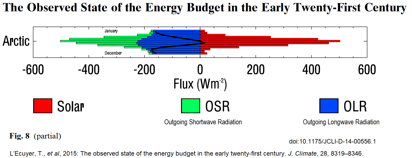
One thing that does NOT cause “Arctic Amplification” is darker water absorbing sunlight that sea ice would have reflected. (That’s a common misconception.) The Arctic is a net exporter of radiation about 11 months of the year, so reduced sea-ice coverage increases heat loss much more than it increases absorption of sunlight.
https://sealevel.info/2015_lecuyer_eeb_jcli_fig7-8.html
Dark water does not absorb EM (aka light). The water is dark due to optical depth of the medium. It absorbs and reflects sunlight due to it being liquid water.
In the same sentence you say “Dark water does not absorb EM (aka light)” and “It absorbs … sunlight”.
?
w.
Global temperature is a averaging error.
Global temperature is physically meaningless.
That too.
T2 is generally called the mid-range statistic, here a special case where there are only two data points available, although a mid-range can also be constructed from data sets that have enough points to calculate a true arithmetic mean. It is not a robust statistic, being particularly sensitive to outliers or erroneous readings. There is no associated Standard Deviation(SD) because one only has the range and the Empirical Rule in statistics says that that SD should be approximately the range/4. SD calculations based on formulas provide answers that do not agree with the Empirical rule or each other. If a data set is normally distributed, than the mean, median, and mode are equal. However, there is no way to determine if the T2 distribution is normally distributed with only two values. As Tim and Jim have pointed out, the sunlit change in temperature is a sinusoid and the night time decrease is exponential. One would not expect the 24-hour distribution to be Gaussian. There is no way to improve the precision of the daily mid-range because it is limited by definition to Tmin and Tmax.
It is a poor statistic to use to try to tease out small variations in a trend. The best that one can say with honesty is what the trend of the mid-range value is in a time-series, which may or may not be useful in describing changes or trends in the climate.
https://en.wikipedia.org/wiki/Mid-range
Thanks for the mention Clyde.
The creation of Tmax and Tmin was never intended to be put to the use it is currently is. At best the measurement uncertainty is a uniform distribution with [(a-b)/2](1/√3). Let’s say a diurnal range (Tmin to Tmax) of 60 to 85. That gives a mean of [(85-60)/2 = 72.5 ±12.5 and the uncertainty is 12.5 / √3) = ±7.2 for the measurement uncertainty.
I ran across a story about a design of a new water plant that was interesting. The river engineer wanted to provide the absolute best estimate possible of the river average depth. So he took the daily average for 25 years and found the average depth was 20 feet ± 6 feet. Wanting to appear very professional he proceeded to divide the SD of ±6 feet by the square root of (25 x 365) and ended up with an SEM of ±0.00066 feet. So the water plant inlet was placed at a depth of 15 feet since the average river depth varied so little. This worked fine for a while but there were long stretches where water had to be pumped because the river fell below 15 feet. It seems the river engineer forgot to tell them that 14% the time the depth would be less than 14 feet, that is the one sigma value.
Does anyone really wonder why averages and incorrect statistical treatment hides so much variance? What do you reckon happened t the bridge that was built with 6 feet of clearance above the average ±SEM?
This doesn’t begin to address the autocorrelation inherited from seasonal changes when the next day is likely to be warmer (colder) depending on spring (fall) changes. Other periodic phenomena such as ENSO and AMO introduce anomalous changes that can affect simple linear regression trends.
Would it not be better to measure temperatures with integrating instruments?
Aren’t sea levels measured that way?
Sam ==> Temperature is measured at automated weather stations more-or-less continuously and reported at six-minute intervals (averaged over the previous six minutes). — this supplies 10 measurements an hour, of which all 240 could be averaged to find the average daily temperature.
this would not be a bad method — as long as the data is not then thrown away — because for many purposes, the daily temperature PROFILE (graph of all the six minute temperatures against time) might be more meaningful
Averages HIDE data.
Just convert everything to Kelvin and add’em all up from midnight to midnight (as you mentioned somewhere already). Viola! degree-day values. An extensive property.
Tim ==> Degree-day values — a terrific idea but no one will do it….for reasons that are not scientific.
Averages hide INFORMATION. More specifically variances in the data. Averages make things appear more concise than they really are when the variance is ignored.
Jim ==> Absolutely correct — I wrote about that aspect of averages in A Beam of Darkness.
“Aren’t sea levels measured that way?”
Yes and no. Classically, sea level gauges were a float hooked to a recording device and placed in a :settling well that filters out “noise” from waves/wakes, etc. A sort of mechanical low-pass filter. Nowadays, a variety of technologies can be used depending on what seems best for a given site. What’s recorded and what has to be averaged/removed in processing. depends on the technology. See https://incois.gov.in/documents/ITCOocean/ITC001/ppts/L2-%20Sea%20level%20measuring%20systems.pdf
Hmm. The maximum number of legs Americans have is 2. The minimum is zero. Hence the N2 number of legs=(2+0)/2. The average American has one leg. It’s science.
It is understood that it is incumbent on those receiving funding via proposals intended to support the global warming narrative that they FIND global warming evidence. Certainly, models show a dramatic warming should be found for latitudes above the polar circle. That was the result of the early 70’s models quoted by Kellogg.
For the summit of Greenland and Antarctica, however, the data support NO significant warming at all. An example, for Greenland, is attached.
I think since the middle seventies we use continuous recording at most ws. The computer then calculates an average for the day.
Anyway, wishing you all a very blessed Easter. Our God is Truth an He is not dead!
https://breadonthewater.co.za/2025/04/16/easter-2025/
The data may be recorded. That doesn’t mean it is used. As far as I know, climate science still uses the (Tmax+Tmin)/2, the mid-range temperature, as it’s “average”. Only agricultural science and HVAC engineering seems to use the integrated temperature profile, i.e. the degree-day values instead of the mid-range temperature.
Henry ==> Amen to that, sir!
I thank the Imaginary Guy In The Sky for causing Schnucks to loss leader their Easter hams for $1.29/#. We will feast on one, kale/brussels sprout salad, Aldi’s buttermilk biscuits, and fishbowls full of Busch beer this PM. Then, heavenly leftovers….
ASOS stations were installed during the 1980’s in the U.S. I would have to dig further to see when the daily average started being reported in the data. I know current data retrieval files have both traditional and 24-hour averages of six-minute data. As Tim points our, the tradition two temperature average is still used in most cases because it “matches” traditional information from the past.
Many of the excuses of bias from CAGW advocates arise from this. It isn’t that the recorded temperatures are inaccurate, they are simply different. Changes in their values so they can be spliced to current records IS NOT scientific. Too many statisticians become familiar with “study bias” that can be removed through mathematical means. It is why there is a current problem with replication in experiments and studies. If you fiddle with the inputs, you also fiddle with the outputs
Henry, Tim, and Jim ==> ASOS (Automated Surface Observing System) and AWOS (Automated Weather Observing System), NOAA uses both for sightly differing automated weather stations, generally record six-minute averages from almost-continuous temperature readings. This method helps smooth out wonky instantaneous peaks and dips, but it does not eliminated them (they affect the six minute averages).
The metric used in all the major Earth-based (meaning, not satellite or weather balloon) temperature data sets is the T2 — (Tmin + Tmax)/2 = Tavg — which is then used upscale for local, regional, national, etc etc averages.
The data is recorded as six-minute values, and the data sets usually contain a separate T24 average as well — but only in the Integrated Surface Database-Hourly (ISD-H, [T24]), available from NOAA, it is used for up-scaled work.
Unfortunately, the Law of Averages was never passed.
A paper published about ten years ago by Cowtan and Way claimed that the polls were warming about 8 times faster than the rest of the planet. That means that the polls today should have warmed about 80 time more than the rest of the planet. (That would be huge unless the average warming for the Earth over the last ten years has been zero.)
Considering that the Earth is cooling (losing around 44 TW – that’s known as “cooling”), talk of “amplification” or “Greenhouse Effect” is just delusion.
Otherwise intelligent, well-educated and highly qualified people cannot seem to understand that thermometers are built to respond to heat, not CO2 or H2O.
Since the Industrial Revolution(s), the world’s population has increased massively, as has per capita energy use. Every single erg of this energy is either converted to “waste” heat, radiated in all directions until interacting with nearby matter like thermometers, or leaving the Earth to space more directly – as visible light, radio waves, etc.
If people wish to believe in fairytales peddled by GHE believers, that is their right. Throughout history people have managed to believe in all sorts of things which didn’t exist. Nothing seems to have changed.
Listen skeptic the average adult human has one large boob and a testicle and there are lots of educated people who think that’s the way it should be so where’s your qualifications?
Well, if you wait a monument, I could emulate Michael Mann and print myself a Nobel Prize award.
Would that be convincing enough?
Thanks, Kip. Good article. Perhaps we should now also talk about the problems associated with 1st-order trends and the bias that can by introduced by the selection of start and end intervals.
Is the trend up, or down over the last decade?
In this plot the start and end were determined by the extent of CO2 data. Clearly the temperature trend would have been higher if I’d fit the range 1975-2016.
I would argue that linear trends aren’t even appropriate for global temperature given that it’s largely comprised of periodic signals for intervals longer than 11 years.
“I would argue that linear trends aren’t even appropriate for global temperature given that it’s largely comprised of periodic signals for intervals longer than 11 years.”
Far too may climate scientists, statisticians, and computer programmers have absolutely no understanding of beat frequencies derived from multiple periodic waveforms. Pete forbid that any of those waveforms actually combine in a non-linear mixing form.
Robert ==> We could, but I try to keep the topics in my essays narrow enough for reasonable discussion.
I would be interested to see a well-written essay discussing the issue you bring up. If you write it and send it to me ( my first name at i4.net ) I try and get it posted here.
Is urban heating a factor?
I expect it would raise the night temperature more than the day temperature. But high latitudes are usually sparsely populated.
Daytime temps are ultimately limited by the ΔT –> ΔT^x (x = 4 for a black body, something less for the earth). That relationship is a negative feedback limiting T
After you complained above about scientists not understanding math, I fear you just massacred the S-B Law. That law says that the magnitude of the radiation output of an object is directly proportional to the fourth power of its surface temperature.
However, that law DOES NOT WORK for ∆T (the change in temperature), or in fact for temperatures in any units but Kelvins.
Sorry,
w.
Scared yet again? Learn some physics, and accept reality. No need for fear.
Pass. First Rule Of Pig Wrestling applies.
w.
Is that what you told X that got you blocked? I can’t say I blame them.
Willis,
I didn’t specify the measuring scale anywhere in my post. So I fail to see what I massacred.
T^4 is for a “black body”. The earth is not a black body. That’s why I said T^x. I don’t have a good estimate for what “x” is but I’m sure it isn’t 4.
If temperature determines radiation flux then the change in temperature, ΔT, will determine the change in the radiation flux as well. If radiation at y = T is
u W/m^2 then the radiation at T + ΔT will be u + Δu W/m^w. What Δu is will be related to the exponential power = x.
The radiation *will* go up faster than the temperature. That is a negative feedback and thus will set a boundary for ΔT at some value.
The real issue is that T and ΔT don’t tell you much about climate. Temperature is not climate. It *is* a factor in climate but there are lots of other variables as well.
I’m sorry, I guess I wasn’t clear. Perhaps an example will help explain.
Let me start with the Stefan-Boltzmann (S-B) law. It says:
Radiation = sigma * epsilon * Temperature^4
where sigma is the S-B constant, 5.67e^-8, and epsilon is the emissivity. For a blackbody, emissivity is 1, and temperature is in Kelvin.
Consider a blackbody at say 15°C, which is 288.15K. Since the emissivity of the blackbody is 1, this has a blackbody radiation of 5.67e^-8 * 288.15^4, which is 390.9 W/m2.
If the temperature increases by a ∆T of say 1°C, which gives a new temperature of 289.15K, the radiation increases to 396.35 W/m2.
From this, it’s clear that for a ∆T of 1°C from a starting point of 15°C, the change in radiation is 396.35 – 390.9 = 5.45 W/m2.
Now, let’s repeat the exercise, but this time starting at 30°C, which is 303.15K. This, in turn, has a blackbody radiation of 478.87.
If this new temperature (30°C) increases by a ∆T of say 1°C, it gives a new temperature of 304.15K, and the radiation increases to 485.22 W/m2.
From this, it’s clear that for a ∆T of 1°C, the change in radiation is 485.22 – 478.87 = 6.35 W/m2 … but the previous ∆T change only increased radiation by 5.45 W/m2.
The thing is, the blackbody radiation is NOT proportional to ∆T^4 as you incorrectly claim.
It is proportional to T^4, so a 1°C rise from 15°C does NOT give you the same answer as a 1°C rise from 30°C
Finally, you said:
Sorry, it doesn’t work that way. It is ALWAYS T^4, and the difference resulting from the Earth not being a blackbody is handled by using the actual emissivity of the Earth, not by varying the exponent as you incorrectly claim.
All of which is why I said you massacred the S-B Law.
Hope this helps,
w.
But what’s your point?
Are you trying to say that adding CO2 to air makes it hotter? Or just trying to be annoying for no particular reason?
Some dimwits are convinced that they can calculate the temperature of the Earth by using the S-B Law! You aren’t one of those, are you?
That would be about as silly as believing that adding CO2 to air makes it hotter!
a. As your own math shows, since this is an exponential relationship and not a linear one, using an average value of (Rmax + Rmin)/2 for W/m^2 doesn’t truly equate to total heat loss.
b. S-B only shows the W/m^2 at the surface of the emitting body. If there is a distance between the source and the measuring device and that distance is some media other than a vacuum, then the path loss of the media will change the W/m^2 received at the measuring device. Every “adjustment” they make to the satellite reading to account for the path loss through the earth’s atmosphere adds measurement uncertainty. And since that atmospheric path loss is highly variable, both in time and geography, the measurement uncertainty can be quite significant.
I’ve never really trusted any radiation budget model for the Earth. Since the radiation profile is related to the temperature profile and the temperature profile is sinusoidal during the day and exponential decay at night (approximately) the radiation profile over 24 hours is more complicated than (Rmax + Rmin)/2. But it’s not obvious that this is reflected in any radiation budget I’ve seen. For instance, at night the radiation profile would follow something like e^(-4λt). I’m too foggy this morning to work that out over a 12 hour nighttime, probably involve a (-1/4λπ) for an average value.
In any case, I sincerely doubt that the measurement uncertainty of the radiation budget is any less than the units digit. Meaning any differential calculated to the unit digit is questionable.
“T^x is *my* shorthand for εT^4.”
After that, I’m gonna pass. You’re off into Racehorse Haynes territory with that one. I’ll come back when you don’t use some secret mathematical “shorthand” in your claims.
Finally, I’m sorry, but the S-B equation does NOT work with ∆T, only with T, no matter what secret shorthand you are using.
Best of life to you,
w.
I’m not sure what you think εT^4 equates to other than something less than T^4, i.e. T^x. T^2 < T^4 with x = 2. T^3 < T^4 with x = 3. All ε does is scale T^4 down so it is something less than T^4. I.e. T^x.
I’m not saying that S-B works with ∆T. I’m saying that T^x goes up faster than ∆T. That should be pretty obvious.
Try to heat a 1’x1’x1/2″ piece of boilerplate out in space (no convection, no conduction) with a propane torch using a disposable tank. What happens? At some point the boilerplate will reach a temperature where it radiates any additional heat input from the torch away faster than the torch can add additional heat. The boilerplate won’t get any higher in temperature once that happens. ∆T = 0 no matter how long you hold the propane torch on the boilerplate.
The sun is that propane torch and the earth is that boilerplate. At some point the sun can’t heat the earth to any higher temperature because any additional heat will get radiated away faster than the sun can input more heat. I.e. ∆T is related to T^x. In the limit ∆T approaches 0. A boundary condition.
You are correct to say that εT^4 = T^x. However, what I objected to is your secret mathematical shorthand.
Yes, as you probably haven’t figured out,
x = log(ε) / log(T) + 4
… but why use that when we have the S-B law which is cleaner, far easier to use, requires less calculation, is long-established, and unlike your secret shorthand, understood by everyone?
Finally, there is STILL no ∆T in either formula, so your claim that
ΔT –> ΔT^x
still has no meaning related to the S-B equation.
You say that your secret meaning for the symbol ” –> ” is “a relationship exists” … but that’s not math, that’s handwaving. WHAT KIND of relationship exists, and how can we measure it?
In addition, you’ve invented your own meaning for a symbol that already has set meanings in math.
In mathematical logic, “A → B” means “if A is true, then B is also true.” This is called a material conditional and is read as “A implies B”. For example, x = 2 → x^2 = 4
In set theory and functions, “f: A → B” means that
f is a function with domain A and codomain B
In calculus, “x → a” means “x approaches a,” commonly used in limit notation.
But using it to mean “a relationship exists” means nothing.
Regards,
w.
Willis,
The bottom line here? I was trying to keep things simple for those who aren’t math inclined. You are nitpicking, pure and simple. Stop it. It’s not attractive.
You still haven’t refuted my assertion that radiation heat loss places a boundary condition on how high T can go. You still haven’t refuted my assertion that an increase in heat content does *not* automatically mean an increase in temperature, at least not when water and water vapor is concerned, thus trying to directly relate radiative flux to a temperature on the earth is a losing battle. It’s way more complicated than that. Most radiative balance models don’t seem to recognize that or allow for it. Just like they don’t seem to recognize the thermodynamic impacts of the earth (both water and land) as a large heat sink.
Thanks. Tim. You claim that replacing
εT^4
with
T^( log(ε) / log(T) + 4)
is “trying to keep things simple for those who aren’t math inclined”??
Got it. But why not say “thermal radiation varies proportionally with T^4” for the math-averse?
Next, you say:
“You still haven’t refuted my assertion that radiation heat loss places a boundary condition on how high T can go.”
Why should I? It’s basically true, with the caveat that it only is true when the amount of heat being added to the system per unit of time is constant.
Next, you say:
“You still haven’t refuted my assertion that an increase in heat content does *not* automatically mean an increase in temperature, at least not when water and water vapor is concerned, thus trying to directly relate radiative flux to a temperature on the earth is a losing battle.”
That’s a multi-part statement. Let me take it a bit at a time:
“You still haven’t refuted my assertion that an increase in heat content does *not* automatically mean an increase in temperature, at least not when water and water vapor is concerned.”
I’m sorry, but an increase in heat content DOES mean an increase in temperature. How much of an increase is calculable from the “specific heat” of the substance being heated, but it’s never zero.
I think you might mean an increase in heat INPUT does *not* automatically mean an increase in temperature, in which case your statement is true in certain warmest parts of the planet, particularly the temperature of the Pacific Warm Pool.
Finally, you say:
“… trying to directly relate radiative flux to a temperature on the earth is a losing battle
I fear you mistake non-linearity or complexity for no relationship. Here’s a scatterplot of solar flux absorbed by the planet’s surface versus the temperature of the surface, gridcell by gridcell.
As you can see, there’s a close relationship, albeit non-linear, between absorbed radiative flux and temperature. You can also see how at the highest temperatures, additional flux does nothing due to a combination of increased radiative heat losses and increased cloud and thunderstorm cooling.
Best regards,
w.
That doesn’t hold at the triple point of water, at least until all the solid phase has changed to liquid.
True indeed, thanks for noting the edge case.
w.
Well, it’s one of the two edge cases.
As much as I dislike the cold, the other edge case would be even more unpleasant 🙂
It doesn’t hold for the liquid to vapor temperature point either. And that point is highly pressure related.
“Got it. But why not say “thermal radiation varies proportionally with T^4” for the math-averse?”
because I didn’t have all day to formulate the post?
“Why should I? It’s basically true, with the caveat that it only is true when the amount of heat being added to the system per unit of time is constant.”
Most people consider the sun’s output to be pretty constant, at least over the short term (daily, monthly, annually).
“I’m sorry, but an increase in heat content DOES mean an increase in temperature.”
No, it doesn’t. I gave you the reason why. Evaporation is a cooling process. Downward radiation that causes evaporation doesn’t actually add heat to the surface, it cools it. It’s why the output temperature from the earth cannot be directly calculated from the radiative flux. The thermodynamic impact of the radiative flux is dependent on the physical process it causes.
“I think you might mean an increase in heat INPUT does *not* automatically mean an increase in temperature, in which case your statement is true in certain warmest parts of the planet, particularly the temperature of the Pacific Warm Pool.”
It’s true everywhere on the surface of the earth that has any water. Remember, evaporation requires an increase in heat energy – which then causes the evaporation. It’s a process. And it happens everyplace you find any water, both in the soil and the ponds/lakes/oceans.
So much of climate science is based on implicit, unstated assumptions. S-B is based on Planck and black body theory. And Planck’s theory is based on a body which is internally in thermal equilibrium. That is *not* the earth. The actual emissivity of the earth’s surface is not a constant, it is a huge heat sink with a widely varied characteristic thermodynamic factor. Yet climate science treats it as such. The emissivity factor is a “measured” and “averaged” quantity based on experimental temperature and radiative flux measurements. This injects a huge amount of measurement uncertainty into the average emissivity factor, yet that uncertainty is *never* included in any calculation of the earth’s temperature based on incoming radiative flux. As I’ve said before, I am of the opinion that the measurement uncertainty is in at least the units digit if not in the tenths digit for calculating the outgoing flux from the earth as well as in calculating the “temperature” of the earth from incoming radiative flux.
“I fear you mistake non-linearity or complexity for no relationship.”
No, it’s because of the measurement uncertainty associated with assuming a constant emissivity based on experimental data being averaged.
“As you can see, there’s a close relationship, albeit non-linear, between absorbed radiative flux and temperature. You can also see how at the highest temperatures, additional flux does nothing due to a combination of increased radiative heat losses and increased cloud and thunderstorm cooling.”
You just repeated what I’ve been saying, just using different wording. If the relationship is non-linear then using a constant average to calculate anything incurs a significant uncertainty. Where exactly does that uncertainty ever get stated? I seem to remember you speaking of a 3 W/m^w difference value – if the uncertainty is in the units digit it will subsume such a value.
Thanks, Tom. One issue at a time.
While the sun’s output is constant, the amount actually hitting the surface varies by minute, hour, day, month, year, century, and millennium …
First, if all the heat entering the area is instantaneously converted to evaporation as you postulate, there is no increase in heat constant.
Next, if the downward radiation is instantaneously converted to evaporation as you postulate, it does NOT cool the surface. The incoming radiation is simply converted to evaporation, so the surface neither gains nor loses heat.
Not true. My graph above clearly shows that over most of the world as absorbed solar radiation increases, so does the temperature.
The claim that climate science treats the earth’s emissivity as a constant is kind of true for the globe as a whole. The reason is that it doesn’t vary much over the months and years, with monthly global emissivity only varying from about 0.973 to 0.977 from 2003 through 2016. Since a difference in the third decimal point is meaningless to many calculations, it is often taken to be constant with virtually no change in the results.
Here’s an example. We measure the global upwelling longwave surface radiation. It varies from 386.4 to 411.5 W/m2, with a mean value of 398.19 W/m2
Using the mean emissivity from 2003 through 2016 of 0.975, this converts to a temperature of 18.17°C. Using the actual monthly variations of emissivity over that period yields a mean temperature of 18.16° … which is why it’s generally taken to be constant for global calculations.
I’m sorry, but you’ll have to give me an example of some scientist “using a constant average to calculate anything”. I’m not clear who or what you are referring to.
Regards,
w.
Rational ==> Normally the high latitudes/Polar Regions basically uninhabited — for UHI purposes.
Climate scientists, statisticians, and computer programmers are all afflicted with the meme of “numbers is just numbers”. Anything you can do with this one set of numbers you can do with any set of numbers and the relationship to the physical world is irrelevant. Thus an “average” temperature, be it a daily mid-range temperature or a global average temperature, can be calculated and used to describe “something”, just don’t look ask what that “something” actually describes in the real, physical world.
An average is just a statistical descriptor of a distribution of numbers. If those numbers don’t describe the physical world then the statistical descriptor is useless in the physical world because it can’t describe the physical world either.
It’s why ag science and HVAC engineering have moved on to using degree-day values. Their results have real-world, real-time consequences that are immediately (within a few months anyway) observable. They have to use data that actually describe the real world for use in estimating heat accumulation and air-conditioning sizing. Fifty years ago the mid-range temperature was the best data both disciplines had available. But not today. Yet climate science remains mired in using old, outdated methods and protocols. They refuse to admit that they could run new analysis methods (e.g. using degree-days and/or enthalpy) in parallel with the old ones – probably because they fear that the comparisons would highlight the inability of the old methods to actually describe physical reality.
I could go on about this for a long time, for instance why doesn’t climate science make more use of soil temperature data in their models? That has at least as much impact on “climate” as air temp taken at 6′ above the ground. Freeman Dyson’s main criticism of the climate models are that they are not holistic. Think about it.
Well said. Climate “Scientists” have never understood the basic points you make about temperatures and enthalpy amongst others, and clearly never will.
Tim ==> Yes, gee, how many times have we hashed all that out here on these [web] pages over the last decade?
If I say here: “One can’t average temperatures!” so many people just go nuts, even though it is true. (Your #3 above). GMST is just idiotic….adding temperatures in degrees, then dividing — grrr.
Thanks, Kip. While you can’t average temperature because it is an intensive property, you can convert it to thermal radiation which is an extensive property, average that, and convert it back to temperature.
Just sayin’ …
w.
Having said that, the differences may be small. If we have two temperatures of say 10°C and 16°C, the average is 13°C. Converting those to W/m2, averaging the two, and converting back to temperature gives us 13.05°C. Interestingly, this is independent of emissivity …
w.
W/m^2 is not enthalpy, i.e. heat. Enthalpy is measured in joules.
For moist air enthalpy is h = h_dry-air + h_water-vapor.
It is enthalpy that really determines climate. It’s the h_water-vapor that differentiates Las Vegas from Miami as far as climate is concerned.
Radiation loss/gain can change enthalpy while not changing temperature (at least very much). Incoming radiation can increase evaporation so that the increase in energy gets pushed into converting liquid water to water vapor instead of increasing temperature. Again, compare Las Vegas with Miami.
So converting temperature to radiation flux and then averaging still doesn’t tell you what you want to know, i.e. the impact on the climate.
Willis, sorry, but that’s just nonsensical.
Only pseudoscientific numbskulls believe that. Adding “thermal radiation” to “thermal radiation” gives you complete garbage – unless you know both the temperature of the emitters, and their emissivities. Completely pointless, in any case – just use a thermometer.
Just sayin’ . . .
Pass. First Rule Of Pig Wrestling applies.
w.
Willis, I don’t blame you for being flabbergasted.
KH, good post.
A fun reminiscence. When MIT Prof. Dick Lindzen kindly critiqued my long climate chapter in Arts of Truth (he actually critiqued the whole book for many hours) we had a brief discussion about Arctic Amplification. He said in 2011, ‘Of course it must exist, since heat flows from hot to cold. BUT we don’t know by how much, since is very complicated.’
Rud ==> Yes, heat must flow from warmer to cooler/hot to cold. But the hot has get be hot first — must exist — in order to create to flow to cold. Heat will generally flow pole-ward — which is not the same as “poles warming four/eight times faster”.
How does the ‘hidden heat’ in the deep oceans sneak past the thermocline?
Kip, you wrote –
Why is that? According to Fourier, during the night, all the heat of the day is lost, plus a little internal heat.
Nothing left to “flow” anywhere.
The Earth is cooling, slowly but surely, losing about 44TW. Energy being lost to outer space, never to be seen again. No pseudoscientific “energy conservation” at all.
Michael ==> The Earth system has many heat-energy moving system — air currents, ocean currents, rising air, falling air, all these move heat around. Warmer equatorial regions supply heat that is moved poleward.
Kip,
No, the Sun provides heat during the day. Air currents are convective , heated from below. Ocean currents are convective, heated from below.
No “heat moving poleward”. Neither hot water nor hot air wander off toward another part of the sphere. Nor does cold water or cold air.
Equatorial regions receive more sunlight, polar regions less.
Lithosphere, aquasphere, and atmosphere are subject to chaos. No more usefully predictable than can be achieved by a smart 12 year old assuming that the future is a mirror of the past.
Presumably, you don’t believe that adding CO2 to air makes it hotter, so I can’t quite figure out what you are trying to say.
Folks, this endless unpleasant kind of pseudoscientific psychobabble such as claiming that there is:
is why I gave up responding to Michael Flynn and simply say:
Here’s what a de minimis search of the subject reveals. References at the end. Note that the Encyclopedia Britannica has a whole section on the subject of poleward heat transfer.
Let me make three requests.
Best to all, here comes the science. Unfortunately, with 20 citations the text is too long for WordPress, so I’ve put the citations in the reply to this post
w.
===
Heat naturally moves from the tropics to the poles through a combination of atmospheric and oceanic circulation systems, transferring approximately 20% of the tropics’ excess heat to higher latitudes [1] [2]. This process moderates Earth’s climate by balancing the surplus of solar energy absorbed in the tropics and the deficit in polar regions.
Mechanisms of Heat Transfer
1. Atmospheric Circulation
-Differential Heating: The tropics receive more intense sunlight due to Earth’s curvature, creating a temperature gradient. Warm air rises at the equator, forming low-pressure zones, while cooler air sinks at the poles, creating high-pressure zones [1] [3].
-Global Wind Patterns: This temperature difference drives large-scale convection cells, such as the Hadley Cell, which transports warm air poleward in the upper atmosphere. The Ferrel and Polar Cells further redistribute heat toward the poles [3].
-Coriolis Effect: Earth’s rotation deflects these air masses, creating prevailing wind patterns (e.g., trade winds, westerlies) that enhance heat transport [3].
2. Oceanic Circulation
-Surface Currents: Wind-driven currents like the Gulf Stream carry warm tropical water northward, releasing heat to the atmosphere at higher latitudes [2].
-Thermohaline Circulation: Density differences from cooling and salinity changes drive deep-ocean currents. For example, the North Atlantic Deep Water formation sinks cold, salty water, pulling warm surface water northward in a “conveyor belt” system [2].
Quantifying Heat Transport
-Atmosphere: Responsible for ~60-70% of total poleward heat transfer via storms, jet streams, and large-scale air movements [3].
-Oceans: Contribute ~30-40%, primarily through surface currents and thermohaline processes [2].
This combined system ensures equatorial regions do not overheat and polar regions remain habitable, sustaining Earth’s climate equilibrium [1] [2] [3].
Citations for the above post, including those not mentioned in the text:
[1] https://bio.libretexts.org/Courses/Evergreen_Valley_College/Introduction_to_Ecology_(Kappus)/02:_The_Physical_Environment/2.02:_Differential_Heating_of_Earth's_Surface
[2] https://www.britannica.com/science/climate-meteorology/Poleward-transfer-of-heat
[3] https://atmos.washington.edu/academics/classes/2001Q4/211/notes_circulation.html
[4] https://www-jove-com-443.vpn.cdutcm.edu.cn/science-education/13664/mechanisms-of-heat-transfer-ii
[5] https://www.terc.edu/buildingsystems/wp-content/uploads/sites/13/2020/07/3.-How-earths-systems-move-heat-energy.pdf
[6] https://www.internetgeography.net/topics/how-do-ocean-currents-transfer-and-redistribute-heat-energy-around-the-earth/
[7] https://www.carbonbrief.org/guest-post-why-does-the-arctic-warm-faster-than-the-rest-of-the-planet/
[8] https://oceanservice.noaa.gov/facts/rossby-wave.html
[9] https://www.e-education.psu.edu/earth103/node/1008
[10] https://www.reddit.com/r/climatechange/comments/1bxi7s9/if_the_poles_are_heating_up_faster_than_the/
[11] https://www.metoffice.gov.uk/weather/learn-about/weather/atmosphere/global-circulation-patterns
[12] https://manoa.hawaii.edu/exploringourfluidearth/physical/density-effects/density-driven-currents/climate-connection-global-conveyor-belt
[13] https://sealevel.jpl.nasa.gov/ocean-observation/understanding-climate/the-earth/
[14] https://meteor.geol.iastate.edu/gccourse/atmos/atmos_lecture_new.html
[15] https://courses.lumenlearning.com/suny-physics/chapter/14-6-convection/
[16] https://rwu.pressbooks.pub/webboceanography/chapter/8-1-earths-heat-budget/
[17] https://open.oregonstate.education/climatechange/chapter/processes/
[18] https://ugc.berkeley.edu/background-content/atmospheric-circulation/
[19] https://www.counterpunch.org/2020/08/04/ocean-heat-from-the-tropics-to-the-poles/
[20] https://www.webpages.uidaho.edu/learn/ecology/lessons/lesson02/2_3.htm
Willis, I don’t blame you for resorting to an Actually Idiotic computer program to try to disguise your ignorance and gullibility.
Sorry, but the fairytale that “Heat” moves from the Equator to the Poles via either the atmosphere, aquasphere or lithosphere is just a lie told to children.
You wrote –
Anyone who uses the word “science” in that sense, doesn’t understand science or the scientific method, as Richard Feynman said.
Unfortunately, Willis, the globe is reasonably globular, so to speak. Every particle of the atmosphere, aquasphere and lithosphere is attracted toward the COG of this globe, no matter whether it is situated at the poles or the equator. Place a spherical ball on a flat surface of the Earth, hot or cold, and watch it stay where it is – no movement.
Whether it is hot, cold, wet or dry. Denser water or air descends towards the COG, no matter where it is. And there it stays, unless moved by a convective process (which involves heating from the bottom, not from the top), in general.
You wrote –
Oh dear, Willis. “Fact by consensus”, is it? Go for it. Maybe you can get people to agree with you that they are equally as ignorant and gullible as you seem to be, but not a single physical fact will be changed!
No GHE. Adding CO2 to air does not make it hotter. The Earth loses energy at around 44 TW. The phenomenon is called “cooling”.
Others can form their own opinions.
I provided 20 citations supporting my claim.
I invited you to provide 20 citations supporting your claim that there is “No “heat moving poleward””.
Instead, you’ve given me your patented mix of insults, handwaving, and bafflegab.
Still waiting … heck, give us 5 citations backing your claim.
w.
Why should I give you anything at all?
People can make up their own minds. You don’t have a problem with that, do you?
Aaaand as expected, Michael runs for the door without making the slightest effort to back up his untrue claims …
w.

Willis, you are being particularly idiotic today. As I said, No GHE. Adding CO2 to air does not make it hotter. The Earth loses energy at around 44 TW. The phenomenon is called “cooling”.
Feel free to quote me on that.
By the way, earlier you wrote –
Tell me, how did that work out for you? How outnumbered did I wind up being? What effect did it have on me?
Haven’t looked at the button. I’m just trying whatever I can to force you to produce even one citation to your ludicrous claim that there is “No “heat moving poleward””.
So far you haven’t had the spine to actually do that, instead resorting to childish insults that I guess on your planet pass for science.
w.
Willis, facts are not established by consensus. Unless you can demonstrate this “heat moving polewards”, it’s about as real as Trenberth’s “missing heat”.
You write –
I notice that in your usual hypocritical fashion you refuse to actually quote these “childish insults”. If you choose to feel insulted, that is your affair.
If you hope that people will feel sorry for you, that’s fine, but I cannot see what you hope to achieve. The equatorial regions will no doubt remain hotter than the poles, and the Earth will continue to cool.
I’m still of the opinion that the Arctic is not a feedback, it is the driver of the 60-70 cycle climate cycle. As such, there is no such thing as “Arctic amplification”. The Arctic temperature is driven by sea ice variability which is part of the Arctic.
Willis had a nice diagram showing how the warming of Earth is lopsided. It is highest near the north pole and falls as one moves south. This is exactly what one would expect if the Arctic was the driver.
We should also see more influence in moderating low temperatures during the warm phase as the Arctic would be producing less cold air. This is exactly what we have seen.
While the measurement system is likely to disagree on the exact amount of change, the overall cause of much of the warming we have seen is very likely coming from the Arctic.
Very nice Kip. I can’t understand the reason for using averages, averages seem meaningless to me. The average high in my hometown for July and August is 85F. A pretty worthless statistic when you are outside in 100F plus. The average low for December and January is 18F. Pretty meaning less when you stay hunkered down inside with a minus 20F outside.
Bob ==> I have answered this question in my various essays on averages and Average Temperatures. If one wants to know what kind of weather one might expect in Jul/Aug in your area, a chart of average Jul/Aug temps would help. This is pragmatic and not scientific, but helpful.
If one wants to beat the world over the head demanding that it stop using fossil fuels because Climate Change, one has to have the rising GMST statistic that shows we are all going to die.
Not necessarily helpful at all, as Bob pointed out.
Possibly fatal, even. The UK Met Office supplied averages to a group of eight SAS troopers who were kitted out to the “average” temperature. Two at least died of hypothermia, four were captured due to being operationally hampered by the cold conditions.
The UK Met Office. Besotted with averages – no appreciation of reality, not enough brains to explain that it’s extremes that kill, not averages.
About as bright as the US Air Force experts, who eventually realised that building fighter aircraft cockpits to suit the “average” pilot resulted in many avoidable deaths, before reality prevailed.
Climate can be said to be the “average” of weather. Just another meaningless description of the past – interesting, perhaps, but completely useless.
On average, of course.
Averages alone can be misleading. That is why the Gorman brothers and I regularly point out that the variance should be reported along with the mean to have descriptive statistics that are useful. If the probability distribution is skewed significantly, then the kurtosis should also be reported. Taking short-cuts in attempting to characterize a data set is fraught with potential problems.
Kip, I’d say that if measurements were used to create temperature chart, then it is the part of the Scientific Method where one records observations before trying to inductively formulate hypotheses. It is the hand-wavers who use undefined qualitative descriptors, and eschew measurements, that need to apologize, not you.
This does seem a rather extraordinary debate. If temperature were a sine wave over 24 hours, one would calculate the Tmax-tmin as 2 while the integral is zero.
The mid-range value would be [1 + (-1)]/2 = 0 as well.
Which is a caution to choose descriptive statistics bounds carefully so that one doesn’t end up with unuseful numbers. If one wants to buy shingles to cover the roof of a shed, the absolute area of the roof is important, not the net variation around the mean.
Richard ==> Thanks for commenting here…the problem with T2 — (Tmin + Tmax)/2 = Tavg — is that temperature is NOT a sine wave over 24 hours
I wrote a pretty good piece on this in 2018 titled: Daily Averages? Not So Fast…
The interesting thing in Zhou and Wang is that using T2 gives quite different results than T24 — and they conclude that T24 is the data that should be used.
If you start with a sphere and a sun that is always over the equator, each point on the equator receives a sine wave from 0 to π of insolation over 24 hours (sunrise to sunset). The average of a sine from 0 to π is 0.637 × peak. This makes the average insolation on the equator 1365 × 0.637 = 870 × 0.7 = 609. Assuming SB. ((609) / (5.67×10⁻⁸)).²⁵ = 322K.
As one moves from the equator to the pole, the insolation follows a cosine function. The average of a cosine from 0 to π/2 is again 0.637. That makes average over the entire 2π (609 × 0.637 = 388). So the average temperature would be (388/(5.67× 10⁻⁸)).²⁵ = 288K.
This is what one would see from a distant point in space with a geosynchronous orbit over the sunlit side and an instrument that gave an average reading. If you moved to a geosynchronous orbit over the dark side, the average temperature would be different due to a polynomial cooling function.
The real question is if averaging these two temperatures provides an accurate radiating temperature. This is where the averaging intensive question arises. I submit the average of the two different functions is a meaningless number.
A check on what the dark side would have to be to arrive at a 255K temperature is the following.
(255 × 2) – 288 = 222K
(288 + 222)/2 = 255K
A 222K is -51°C. Pretty doggone cold.
Remember, these are ideal calculations. Lots of other things to address such as eccentricity, elliptical orbit, sun variations, clouds, oblate spheroid shape, etc
As I reread this, maybe a better explanation might be worth it.
Assume you have an orbiting satellite that remains over the equator and is centered over the sunlit side. Then another similar satellite over the dark side. As above the sunlit side should read a 322K radiating temperature on the sunlit side. What would the dark side need to read to make an average of 255K? (255 x 2) – 322 = 188K. That is a -85°C. Again, pretty cold.
Mmm … here’s the result of a real-world example of your thought experiment … the temperature of the moon.
Best to you,
w.
https://wattsupwiththat.com/2020/02/13/fun-with-lunar-temperatures/