From Dr. Roy Spencer’s Global Warming Blog
Roy W. Spencer, Ph. D.
In a recent post I used our new Urban Heat Island (UHI) warming estimates at individual U.S. GHCN stations having at least 120 years of data to demonstrate that the homogenized (adjusted) GHCN data still contain substantial UHI effects. Therefore, spurious warming from UHI effects is inflating reported U.S. warming trends.
The data plots I presented had considerable scatter, though, leading to concerns that there is large uncertainty in my quantitative estimates of how much UHI warming remains in the GHCN data. So, I updated that post to include additional statistics of the regressions.
A Simple Example: High Correlation, But Low Confidence In the Regression Slope
The following plot of a small amount of data I created shows what looks like a pretty strong linear relationship between 2 variables, with a regression explained variance of 82% (correlation coefficient of 0.91).

But because there are so few data points, there is large statistical uncertainty in the resulting diagnosed regression slope (21% uncertainty), as well as the regression intercept (which is diagnosed as 0.0, but with an uncertainty of +/- 0.94).
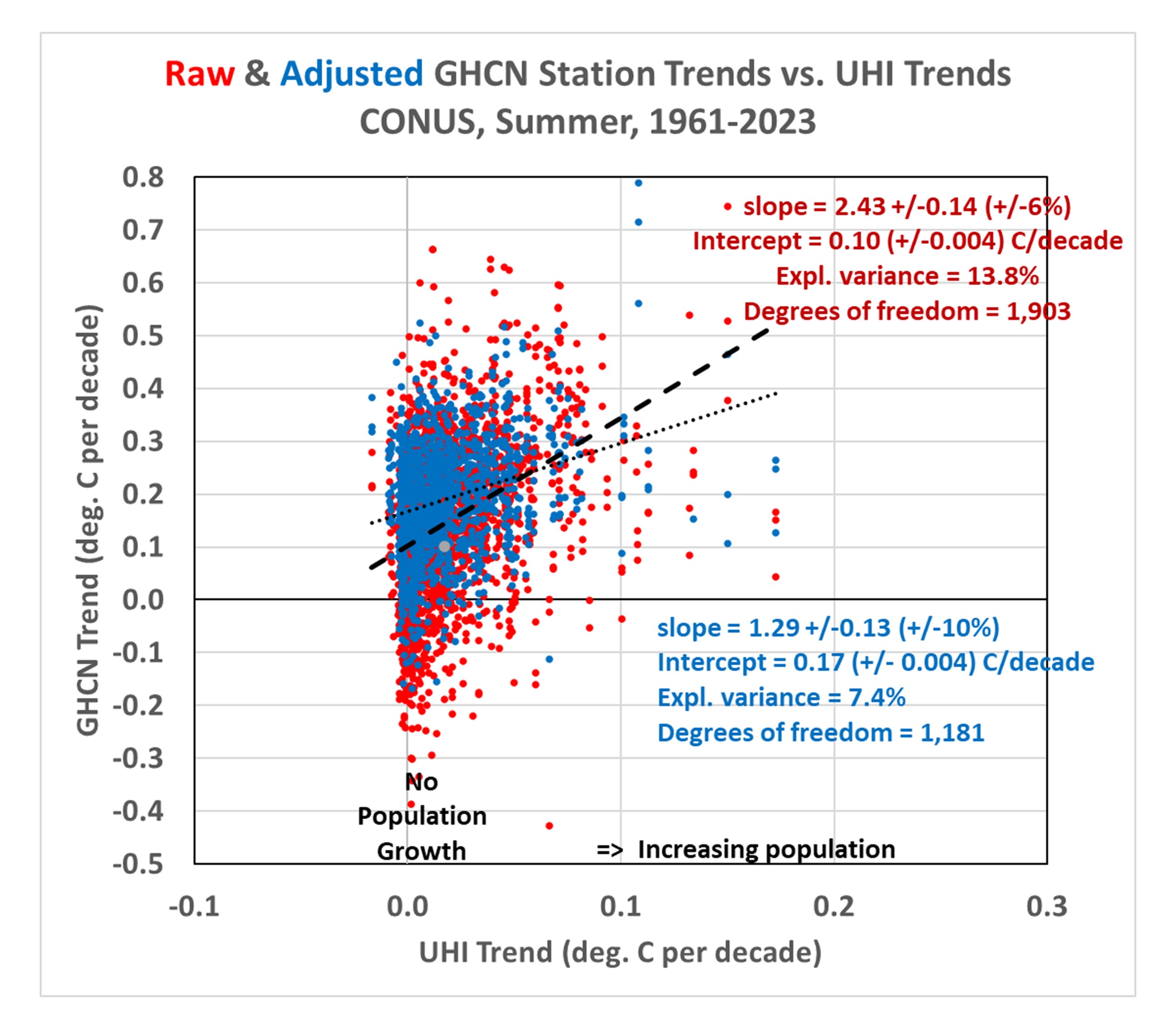
Now let’s look at the third data plot from my previous blog post, which demonstrated that there is UHI warming in not only the raw GHCN data, but in the homogenized data as well:

Importantly, even though the regression explained variances are rather low (17.5% for the raw data, 7.6% for the adjusted data), the confidence in the regression slopes is quite high (+/-5% for the raw GHCN regressions, and +/-10% for the homogenized GHCN regressions). Confidence is also high in the regression intercepts (+/-0.002 C/decade for the raw GHCN data, +/-0.003 C/decade for the homogenized GHCN data).
Compare these to the first plot above containing very few data points, which had a very high explained variance (82%) but a rather uncertain regression slope (+/- 21%).
The points I was making in my previous blog post depended upon both the regression slopes and the regression intercepts. The positive slopes demonstrated that the greater the population growth at GHCN stations, the greater the warming trend… not only in the raw data, but in the homogenized data as well. The regression intercepts of zero indicated that the data, taken as a whole, suggested zero warming trend (1895-2023) if the stations had not experienced population growth.
But it must be emphasized that these are all-station averages for the U.S., not area averages. It is “possible” that there has (by chance) actually been more climate warming at the locations where there has been more population growth. So it would be premature to claim there has been no warming trend in the U.S. after taking into account spurious UHI warming effects. I also showed that there has been warming if we look at more recent data (1961-2023).
But the main point of this post is to demonstrate that low correlations between two dataset variables do not necessarily mean low confidence in regression slopes (and intercepts). The confidence intervals also depend upon how much data are contained in the dataset.
Portland Oregon from 1859 to 1941 had its weather station in downtown Portland. By 1941, it showed a regular increase throughout. In other words, it was a continuous increase from the beginning to the end. Then, in 1941, the official weather station was moved to the Portland Airport, which was some 15 miles to the east, and sparsely populated. There was a sharp drop in recorded temperatures at first. (a spike down.) The curve of temperatures since 1941 is almost identical to that of 1859 to 1941. I used to be able to find and document that change, but for some reason, those records cannot now be found. The portland airport now is an international airport, and industry has built up around it. The number of jets has probably quintupled, but the weather station is trusted as the record of ‘climate’. SMH!!!
A nice microcosm of the “inconvenient truth:” Scientifically speaking, the instrument temperature record is crap in terms of being fit for measurement of any “climate” signal.
And when the data is crap, so is the science based on it.
Your station would be typical. A fixed station’s temperature will normally show an increase over time. It is due to the fading of the paint on the Stephenson screens, build-up of dust, spiders making webs in the corners of the enclosure, surrounding trees growing year by year and blocking some of the view of cold sky on many nights…. Followed at some point by cleaning and repainting and a tech recalibrating the sensors a bit on the high side to avoid explaining why the cleaning made so much difference.
Add all the stations together and you have continuous “climate warming” from systemic error….with probably some confirmation bias thrown in.
The story is not worrisome- easily attributable to humans making convenient choices.
“ I used to be able to find and document that change, but for some reason, those records cannot now be found.” is where I get suspicious. Publicly funded research seems to have become privately owned. It may always have been that way, I don’t remember. Here’s where the government charter should have been written “we will pay for your station and you shall publish the unmodified data”. THus I blame my own government (“us?”).
“So it would be premature to claim there has been no warming trend in the U.S. after taking into account spurious UHI warming effects.”
It would also be pointless. Population growth actually happened. There is no use trying to correct temperatures back to an unpopulated US. You can, if you want, try to say that some fraction of the warming was due to growth. But you can’t say, as a matter of measurement, that it didn’t happen.
The key question is whether the regional average is distorted by too many UHI-affected stations in the sample. But this analysis won’t help there.
The Probity, Provenance and Presentation of temperature “data” are abysmally flawed.
Why anyone with half a rational brain would put any trust in these “constructs” is beyond me.
And then to use these constructs as any sort of guidance for appreciation and/or understanding of the behaviors of the numerous unique climates around the globe is infantile reasoning.
Throw it all away and hire a soothsayer ffs.
Better chance of getting anything right that way.
The question is whether UHI is leading us to believe that global temperatures are rising when in fact they are not. When all that’s happening is that the instruments are showing changes in local temperatures due to purely local causes, while the general temperature of the planet or nation has not changed.
Its like you have 100 years of readings from the shore of Lake Michigan, and use them as a measure of the temperature of the lake. In fact, the temperature of the lake has not changed at all, but the readings have soared, because Chicago arrived with all that concrete. For instance.
The argument is that ‘we’, ie humanity, must keep the average of readings of worldwide temperature gauges from exceeding a 1.5C rise.
Why? What is so important about these particular points where we are measuring? In the UK the previous summer there was complete hysteria about high temperatures measured at places like air bases. Or winds measured at the most exposed places anyone would find.
Why do we care if RAF Marham is recording 40C for a few hours because planes are taking off more than usual this July? Or because some exposed clifftop in the west of the country measured a high speed gust?
To keep up the argument you have to believe that the readings are comparable throughout the series, and not influenced materially by anything other than rises in CO2. Otherwise they are just not measuring the variable of interest.
So now you are saying it makes no difference whether the cause of an apparent warning trend is due to CO2 concentrations in the atmosphere, or whether it is caused by urbanization and development. Because if that is what you’re saying now, you could have spared us all the argumentation over the last 40 years and just said, humans are heating the planet, and unless we ll go back to living in caves again, it’s unavoidable.
You guys .. you just keep slipping and sliding and squirming around like greased pigs, refusing to allow yourselves to pinned down on any of your assertions when the data says different.
No, Duane, that isn’t what Nick is saying here. It is what he’s said elsewhere, but not here.
OK, this is clearly dogpiling on Nick just because he’s Nick. Nothing he said here is unreasonable. Let’s try to be better than that.
For probably the first time, I agree with you.
Applying statistics to meaningless data is a waste of time
USCRN allegedly has no UHI
Spencer ignores USCRN
UAH covers the entire planet which is 29% land and less than 1% is urban land. That means UHI increases could affect anywhere from 1% to 29% of Earth’s surface. Far from 100%. No one knows how much. Spencer ignores his own UAH data.
NASA-GISS has an adjustment for global UHI. About five years ago I wrote an article on the subject. Their adjustment was tiny — only about +0.05 degrees C. warming caused by increased UHI over 100 years.
Why so small?
Because NASA-GISS claimed less UHI at almost as many land weather stations as they claimed had more UHI.
I recall that urban stations that were moved to rural or suburban airports were considered to have reduced UHI. That may be true for a year or two, but economic growth around airports and more jet traffic most likely soon caused an increasing UHI trend.
Exactly. USCRN is warming faster than the adjusted US data!
USCRN starts in Jan 2005. As of September 2024, its linear warming rate is +0.41C/dec compared to the (adjusted) ClimDiv rate of +0.34C/dec.
For comparison, over the same period, Dr Spencer’s UAH_USA48 data is currently +0.33C/dec; very close to the adjusted ClimDiv rate.
“UAH covers the entire planet which is 29% land and less than 1% is urban land”
It isn’t land/sea area that matters but the mix of measuring stations.
How many temperature sensors are on the 29% land versus how many on the 71% water and how, again, are they averaged?
There are essentially zero air temperature sensors on the oceans, ARGO measures water T.
As a point of interest how many stations in the Kalahari or Sahara?
Probably only where airports exist.
Correlation and confidence are independent are they not? One shouldn’t imply the other.
A tricky issue here is that the station trends likely cover different periods. I don’t think you’ll find 1905 US stations with good coverage from 1895 to now. And it is likely that rapidly growing places acquired their stations more recently. The trend plotted will be for this more recent time, where the warming overall was more rapid. Conversely places with stagnant population are more likely to have their stations cease to report. So their trends are from the earlier, non-warming time. But they all go into the regression with no allowance for that.
Certainly something that needs to be more rigorously addressed.
Very interesting. I am surprised this hasn’t been done years ago.
Rather than typical area gridding as a next step, consider CLT sampling then oversample the data. The result should be more robust.
Sampling is not really the issue. These are measurements where a comprehensive calculation of a “metric”, for lack of a better term, is being done. Declaring the final metric as a “temperature” requires following metrology methods and not statistical sampling methods.
Measurement observations are grouped into a random variable whose probability distribution determines the standard values for a stated values and its uncertainty. For temperatures, there are no multiple observations of each measurement. When looking at daily Tmax temps, these observations are a population. You can’t have 100 Tmax values in a month. Consequently, the mean (assuming a normal distribution) does not need to be estimated, it is the mean. Sampling by groups, or randomly, or stratification gains one nothing.
The sparse data with unknown pdf is a problem.
My stats prof years ago placed his faith in the eyeball over the numbers.
If the eyeball can’t spot the relationship on an XY graph, it doesn’t exists.
Well, this was evidently a response to my previous comment.
Lets do some common sense basic probability thinking before any fancy BLUE theorem statistics..
The posted x/y abscissa intercept must be highly uncertain. The slope must be highly uncertain because there are so few.far away outliers. No fancy T statistic based on more data can salvage those fundamental visual problems.
Despite the fancy math, statistics is at heart simple probability common sense.
I can’t help but wonder what happens to the regression lines if all the data > 0.1 were removed — seems like it wouldn’t be much more than an average.
Yes, I suspect that the few data points out to the right are having an undue influence on the slope and intercept.
Surely Nick Stokes, Roy Spencer, Anthony Watts and a few others here can come up with an agreed list of 100 weather stations with a hundred years of records that haven’t been tainted by city growth, re-location etc. And then look at the trend.
The New York Times reported on January 26, 1989 : “US Data Since 1895 Fail To
Show Warming Trend”
“After examining climate data extending back nearly 100 years, a team of
Government scientists has concluded that there has been no significant
change in average temperatures or rainfall in the United States over that
entire period.
While the nation’s weather in individual years or even for periods of years
has been hotter or cooler and drier or wetter than in other periods, the new
study shows that over the last century there has been no trend in one
direction or another.
The study, made by scientists for the National Oceanic and Atmospheric
Administration was published in the current issue of Geophysical Research
Letters. It is based on temperature and precipitation readings taken at
weather stations around the country from 1895 to 1987. ”
Why not look a that data set again?
Places, for example Dallas TX and Phoenix AZ, have changed since January 26, 1989
Yes, but that data set has not. The suggestion is to revisit the data from 1895 to 1987, unless I have misunderstood altipueri’s note.
AI uses huge amounts of data, for the purpose of high predictability of a process, such as writing an article, doing an interview, bots sounding like humans in their responses to additional questions, plus the data has to be accurate
Compare that to temperature measurements taken throughout the world, and using them. to conclude there was 1.23 C of warming since 1900.
Such a statement is off the charts ludicrous, because the temperatures are inaccurate by about the same amount, especially during the early years
Or simply just nonexistent.
0.8 C +/- 1.5 C
Even accounting for urban heat island effects, the range of those effects is very wide and is due to more than just urbanization, and very much depends upon where the current and historical temperature readings are collected.
In a place like Las Vegas NV or Phoenix AZ with relatively low ground cover by deciduous trees and turfgrass, the UHI will be relatively higher. In places with concentrated paved development such as areas with major vertical development (think Manhattan or Miami-Fort Lauderdale), or with major arterial road intersections, freeway intersections and exits, or with large institutions with large parking lots and buildings (like factories, shopping malls, etc.), or with major regional airports, the UHI will be greater than in the low rise residential suburbs with lots of turf grass and deciduous trees. It’s all urbanization, but it isn’t the same.
It also matters even in completely undeveloped areas – those that have large expanses of bare rock or mostly unvegetated desert surfaces have a large rural heat island effect, and they will be affected mostly by how much cloud cover there is (presumably all such areas have relatively low rainfall). While undeveloped areas that are mostly forest (deciduous or conifer) or grasslands will have different non-urban heat effects.
The later matters because the UHI for dry places, despite heavy urbanization, may not be all that great because the undeveloped natural ground performed much like rooftops and paving in terms of absorbing daytime heat from sunlight then giving it back at night.
There is no one “urban heat island” effect, but a very large range of same.
What needs to be determined is the net impact of significant urbanization over the last several hundred years on Earth’s average atmospheric temperature … and subtract that impact from whatever the warmunists are blaming on elevated CO2.
One factor in UHI is the increased surface areas of buildings relative to the base foundation.
Consider a 1 m^2 of concrete. Now consider a 1 m^3 hollow cube with walls of that same thickness The cube has 5x the surface area as the slab. More surface to absorb energy. More surface to emit energy.
Dr. Spencer, your articles are instructive. I read them several times to extract the information you provide.
I have one nit to pick however. The regression lines you are using assume the data points are 100% accurate, i.e., no uncertainty whatsoever. That is far from what measurement uncertainty gives you.
Anomalies should carry the measurement uncertainty of the random variables used to calculate them. Since those random variables are subtracted, the variance is added using RSS. Looking at NIST TN 1900 Ex 2, the expanded uncertainty is ±1.8°C. This is a minimum value for a monthly anomaly. One should also recognize that the NIST example assumed that measurement uncertainty was negligible.
Creating a new random variable called “decadal average”, one ends up with a random variable containing 120 values and whose individual uncertainties add in RSS. That uncertainty should then be added to the dispersal of the 120 values.
The operative statement from the GUM is:
F.1.1 Randomness and repeated observations
Repeated observations of a single sample is done when the monthly anomaly is calculated. Differences among samples is the standard deviation of the 120 values.
“I have one nit to pick however.”
I’ve lots of nitpicks, but as usual your one has no relation to the issues.
This is about regression lines, and in fact the regression line of sets of slopes, yet for some reason you are obsessed with the uncertainty of monthly anomalies. Which is odd as Spencer isn’t using anomalies, and even if he was, any slope would be the same regardless of the base temperature.
“Looking at NIST TN 1900 Ex 2, the expanded uncertainty is ±1.8°C.”
For one month, for one specific station with incomplete data. And as I keep pointing out the uncertainty is not the uncertainty of the actual average temperature of the month. It’s the uncertainty assuming each daily maximum is an iid random variable. It’s the uncertainty of what might be the underlying temperature for that month, not the measured temperature.
“Creating a new random variable called “decadal average”, one ends up with a random variable containing 120 values and whose individual uncertainties add in RSS.”
Completely wrong, and if you actually understood 1900 Ex 2, you would understand why. Each monthly average is a value from a random variable. The uncertainty of the average would be calculated in the same way as you did for the the monthly value. The standard deviation divided by √120. But then you have to allow for the lack of IID given the seasonal pattern. Use anomalies for each month for example. But you definitely do not want to just add the individual uncertainties, that’s just going to give you the uncertainty of the sum of the 120 months, not the average.
And none of this has anything to do with the uncertainty of the regression. That’s already taking into account the variation of the data around the regression line.
The uncertainty of the regression line is no better than the uncertainty of the data used to create it. End of story.
Draw a line between two points. Say (1,1) and (10,10). Now let’s say each value has an uncertainty of ±1. That means the line could be from (0,1) to (10,11) as an example. There are several other options too. How uncertain does that make the line?
So tell us why uncertainty doesn’t affect a regression line in this manner. Your assumption is purely based on 100% accurate data. No one that has dealt with measurements will buy that.
You’ve no excuse for not understanding this by now. A linear regression is not a case of joining two points. It’s the best fit (for some definition of best) through all the points. The uncertainty is based on the probability of all the points arising from a given line. The more points the less uncertainty. This is the point Dr Spencer is making in this post.
However, the point I was making is that this uncertainty depends on the entire variance of the points about the line – not just the uncertainty of the individual points. In this case the points are varying by several tenths per decade. This variation already includes any variation caused by the errors in the individual points, but is mostly due to actual variance in the trends of the individual stations.
I’m not going to waste time trying to educate you.
Each number there has measurement uncertainty. That measurement uncertainty WILL modify the best fit regression line equation. Every combination of possible stated values will change the equation of the regression line. That is the uncertainty in the slopes and intercept resulting from measurement uncertainty.
If you want to ignore it, that is your prerogative.
Try educating yourself. You could start with 8.4 of Taylor which explains how to determine the uncertainty of the regression line. You can find the same equations in different forms in any decent stats book.
What you say is not wrong, every error contributes to the uncertainty – but that means the uncertainty decreases with sample size. What matters is the deviation of the residuals. That deviation includes the measurement errors – it is not ignored. But in cases like this, where there is a lot of natural variation, the effect of measurement errors will only be a tiny part of that variation.
The sample size of each measurement IS 1 (number of 1). There is one reading of one temperature. n = 1. √1 = 1.
If you collect multiple temperature readings of different temperatures into a random variable look to the GUM Section 4.2 for finding the dispersion of measurements surrounding the mean of the random variable.
See what the GUM Section F.1.1.2 says:
Look at the bolded part. A component of variance arising from differences among samples. What do you think TN 1900 does?
Look at an uncertainty budget. Tell us what repeatability uncertainty is and what conditions are used. Think measuring the exact same thing.
Then tell us what reproducibility uncertainty is and what conditions are used.
Measurement uncertainty isn’t about sampling, it is about probability distributions and the ability to define internationally agreed upon definitions of what intervals should be used to describe the dispersion of measurements.
“The sample size of each measurement IS 1 (number of 1).”
I’m so glad you’ve given up pretending to teach me. This tiresome nonsense is just as wrong as it was every other time you’ve used it. If you don’t like the term sample size, just call it the number of observations, of number of data points.
In this case the data points are the slopes the temperature trend of individual stations measured over 130 years, compared with the trend in population over the same period. There are about 100 individual stations, and that means the sample size is 100. That is the N that goes into the calculation for the uncertainty of the trend lines in Spencer’s paper.
“Measurement uncertainty isn’t about sampling, it is about probability distributions …”
What do you think the uncertainty of the trends are? They are probability distributions, based on the assumed probability distributions of the residuals. These distributions include any errors resulting from measurement uncertainties.
This is all standard, basic, statistics, and there are lots of reasons why I think Spencer’s analysis is dubious. But you can’t hope to understand this unless you understand how the uncertainties are calculated, and why measurement uncertainty in daily measurements are not going to be a big issue.
Until you can admit and deal with the fact that the numbers you are dealing with to create trends have large uncertainties, you will always fall back to the claim that trend uncertainty is based on the residuals.
You have no appreciation of physical measurements nor their measurement uncertainty. If you did you could quote the sources from the GUM that support your assertions.
If you would read Sections 8.3 and 8.4 in Dr. Taylor’s book you would see how to calculate the uncertainty of σᵧ, the uncertainty in the “y’ variable and how it effects the linear equation uncertainty. As much as you would like to compare the data uncertainty to the residuals of 100% accurate data points, that just isn’t the case.
“If you would read Sections 8.3 and 8.4 in Dr. Taylor’s book…”
You mean the bit that I keep telling you to read. The part that tells you how to calculate the uncertainty of the regression line.
“…you would see how to calculate the uncertainty of σᵧ,…”
I know how to calculate σᵧ, it’s the standard deviation of the residuals. And in the case of Taylor’s examples the measurement uncertainty – given that this is assumed to be the only source of error.
It effects the uncertainty of the slope, because that’s given by
√[σ²ᵧ / Σ(x – x̄)²]
The denominator is equivalent to N ✕ Var(X), hence the more observations the smaller the uncertainty. Just as Spencer is trying to explain.
(Granted, Taylor doesn’t make the equation clear with his Δ symbol, but if you follow the algebra you should see his equation is the same as the above.)
If you don’t agree with this, you need to explain exactly how you would calculate the uncertainty of a simple linear regression slope, and provide some reference.
No, the part that shows you that Δy, the uncertainty in the y values, modifies the y-intercept of the regression equation, thereby moving the regression line.
Technically, since you are using a time series, the x-axis is made up of counting numbers that have no uncertainty, therefore the slope does not change.
Do yourself a favor and change the y-intercept value by a measurement uncertainty value of ±0.5°C and see what range of values are possible with your simple regression.
Lastly, Dr. Taylor’s discussion of regressions is most pertinent to those where “x” and “y” have a linear functional relationship. Show us your functional relationship of time and temperature. Maybe, just maybe, you should learn about time series analysis to get a better understanding of what you are actually calculating when time is the independent variable.
Why not do what I said, and explain exactly how you think the uncertainty should be calculated? There are so many misunderstandings and distractions in this one comment, I’m not sure if it’s worth pointing them all out.
“No, the part that shows you that Δy, the uncertainty in the y values, modifies the y-intercept of the regression equation, thereby moving the regression line.”
Firstly, I was talking about the slope of the line not the intercept. That’s what matters to Spencer’s argument.
Secondly, I’ve already given you the equation for the uncertainty of the slope, and it shows how σᵧ affects the uncertainty. The bigger it is the more uncertainty. But the bigger the variance in X, and the more observations, the less uncertainty. This is the point Spencer makes, and you keep dancing around.
Thirdly, for the uncertainty of the intercept the equation is
√[(σ²ᵧ Σx²) / NΣ(x – x̄)²]
As with the uncertainty of the slope, the uncertainty of the intercept decreases with the number of observations.
“Technically, since you are using a time series, the x-axis is made up of counting numbers…”
We are not “using a time series”. Spencer’s regression is comparing temperature trends to population trends. The x axis is the population trend for each station, not time.
And in a time series the x-axis can be in whatever numbers you want, integers or real numbers, depending on how you want to measure time.
“…that have no uncertainty, therefore the slope does not change.”
You have an amazing ability to demonstrate you don’t know what you are talking about. All simple linear regressions assume there is no uncertainty in the independent variables. This does not mean that the “slope does not change”.
This does raise one of my concerns about Spencer’s regression. As his x-axis has uncertainty, it may well be better to use Demming regression.
“Do yourself a favor and change the y-intercept value by a measurement uncertainty value of ±0.5°C and see what range of values are possible with your simple regression.”
What has that got to do with anything? You can;t change the y-intercept by ±0.5°C, because that’s not the units it’s measured in. If you mean ±0.5°C / decade, then the slope will be radically altered. But it’s a meaningless exercise.
Here’s a wild guess as to what the line would look like if you fixed the intercept at +0.5°C / decade. It would certainly show there is no warming from UHI.
“Lastly, Dr. Taylor’s discussion of regressions is most pertinent to those where “x” and “y” have a linear functional relationship.”
Indeed, the assumption of this linear model is that the relationship is linear. That’s one of the main assumptions of a linear regression. It would certainly be a good idea if Spencer tested against other models.
But the relation ship does not have to be functional. That’s why there is an error term. A simple linear regression model is of the form y = A + Bx + ε, where ε is assumed to be a random value – hence not a functional relationship.
“Show us your functional relationship of time and temperature.”
Again, that is not what Spencer’s argument is about. He’s comparing temperature trends to population growth. (What he calls UHI trend, is I think modeled on a regression between trend and population.) It is definitely not a functional relationship, as should be evident from the graph.
“Maybe, just maybe, …”
You should try to explain how you think this should be done, rather than assuming you understand this better than everyone else. And Maybe, you should try to understand that this is not a time series.
Looking closely at the UHI graph there is something goofy going on. The data is clumping, leaving gaps on the X axis. This strongly suggests there is a non random element in the data which violates the statistical assumption you are dealing with a random sample.
Your sample does not look random to me.
I still would oversample the data randomly and see how it affects the results.
It has been my experience that one sees such vertical columns when the data have low precision or are rounded off to far fewer significant figures than the x-axis increments. That is, if one plots integers with a continuously varying abscissa, you will get the effect seen in Roy’s graph.
That was my thoughts also. LOP errors. Or degrees C/F conversion errors.
In any case there is a hole in the X axis at 0.06 or so.
Myself I would be looking at that because it is unexpected.
Might be something interesting.
Dr Roy Spencer,
Much as I would like to agree with your analysis, I have a problem or two to report.
Australia is good for UHI studies because there are many candidates for “pristine” stations, that is, those so distant from people and action that they have no plausible, measurable UHI effect at all. As well, there are numerous lengthy official BOM records to tap.
Here is a graph of the temperature/time series for the 45 longest, most pristine sites I could find. This version shows daily Tmin that the graphing program has converted to smoothed annual presentations for available years. There are some artefacts caused by missing data, but let’s skip that for the moment.
http://www.geoffstuff.com/pristtmin.jpg
An immediate impression is noise. These stations do not show any feature in common that might allow a definition of “pristine”. Some stations show upward peaks at the same time that others are downwards.
The next feature is the trend. It is far from constant, with the highest value in deg C per century being 3.1 deg C per century equivalent and the lowest being 0.15.
….
Please correct me if I am wrong, but your method of UHI analysis seems to assume that differences in trend are related to population alone (or mostly). This has to assume that you have not included trend variations from unknown effects, perhaps because you assume that they are small. (As in a smooth baseline). This Australian data shows trend differences are not small. (I accept that your US data might be of different quality).
Further, you seem to assume that trend differences are related to population changes at unspecified times. Some of this Australian data (if there were UHI effects) has peaks and troughs all over the place, sometimes more than one large peak in the data from one station. This presentation in my link has no reasons to explain why the peaks or troughs are absent, present solo, or multiple. I am suggesting that the same roughness of texture is present in your USA station data and that it puts a rather big question mark over your method.
Do you have any eqivalent USA data to compare with mine?
All the best Geoff Sherrington
Geoff,
You are looking at variance in the data. That isn’t really noise. Think of volume variation in an audio waveform. The variance is what contributes the the uncertainty in a measurement. In other words, the 1σ and 2σ variations tell one the variation in measurements that can be considered to be within those intervals.
Jim,
In 1950 when I was 10, my Dad was into am radio for domestic use after his war experience. The small house was filled for hours with radio noise of various quality. One type was sound like music or speech of varying fidelity that waxed and waned in intensity over cycles from minutes to parts of days like afternoons to nights.
This is how I see this “noise”. There is an am frequency on a carrier wave that varies in intensity over months. This is not a conventional view. I am floating it to see if it has support.
Geoff S
I have been a ham radio operator since I was 14, 60 years ago. Believe me I have heard everything you mention.
Noise in a radio signal is extraniously generated EM waves that combine at a receiver. The non-signal EM can mask the wanted signal by being “stronger” when demodulated. When this occurs, the wanted signal is lost. AM signals are very prone to this.
The key here is unwanted non-signal interference that has the same properties as the signal. From a temperature standpoint, what would be noise? UHI. Poor siting. Poor maintenance. Anything that generates a portion of a temperature reading that modifies the intended measurement. That is ultimately, all the uncertainty categories contained in an uncertainty budget.
Variation in temperature readings is not noise. Seasons are one example of a variation in temperature that are not noise. Seasonal variation IS THE SIGNAL.
This is different from what statisticians call noise. To a statistician, residuals of a regression are noise. Kurtosis and skewness are noise indicators. Basically, any data that does not perfectly fit into a probability distribution that is known a priori.
How does a statistician eliminate statistical noise? Averaging is a big method. You arrive at just one number that has no indication of the underlying variation, i.e., noise. If you average averages, you eliminate even more statistical noise. If you create anomalies, you reduce the magnitude of any variation thereby reducing statistical noise. Then you can divide the indicator of dispersion, σ, by the √n to reduce the noise figure even further. The original variation in the signal becomes obscured under layers of calculations.
The statisticians here need to realize measurements and metrology embrace the variations. The GUM even quotes that you must state the variation (uncertainty as a standard deviation) when quoting a stated value of a measurement. Propagating those variations throughout any all calculations is necessary to adequately address the original variations in measurements.
Metrology is the science of measurements. The GUM was developed as a primer containing methods to arrive at internationally agreed quantities of stated values and dispersion around those stated values. Probability distributions are used to calculate the stated values and standard intervals of dispersion. That is where the use of statistics(?) ends when dealing with measurements descriptions.
Jim,

My idea is that there are unrecognized or poorly recognized factors that cause peaks and troughs in the time series that I show. The signal that is sought, the temperature, is moved up and down at a timing of months peak to peak, guaranteeing that the graphs I show have essentially no straighht line sections of any significant duration. The type of interference (for ham radios, might be level of atmospheric moisture that the radio signal passes through, more, more). The type of mechanism includes Anthony Watt’s paint quality on the thermometer screen, but I favour other drivers that so far are beyond my imagination.
I have another study of Melbourne and 20 or more stations in its suburbs and outlying villages up to 40 km way. I have applied corrections for altitude (lapse rate) and latitude to try to make them more the same, but one station Coldstream, persistently captures the news as the coldest night around Melbourne. I cannot imagine or suggest why it is persistently colder. It is almost as if Stevenson screens and other screens have a feature that causes month to year length ups and downs. Almost as it trees were casting shadows with seasonal influence as well as gardeners and tree trimmers. I cannot lay down my winning hand and cry Trumps yet, but I cannot fold my hand on the idea of this puzzling interference. It is in the signals, but who can explain, explicitly and site by site, why the signal goes up or down on any specified date, which might not be the same answer as another station gives 5 km distant.
Geoff S
Many of the things you mention are systematic in nature, even those that are seasonal. Seasonal uncertainty is entirely possible and will cause various times to be incomparable without adjustment. This is where time series analysis steps in and is what should be used to arrive at temperature trends. Stationarity is something that should be accomplished before making conclusions about time series data.
Doing regressions on averaged data is a joke. During my career at the telephone company we went from frequency multiplexed carrier systems to time division carrier systems. Frequency multiplexing worked kind of like an AM/FM radio. The incoming signal was applied to a number of filters that only passed certain bands of frequency thereby breaking out an individual conversation. These were pretty much limited to about 12 conversations per cable.
Time division multiplexing was a whole new ballgame based on sampling a conversation at a given rate with discrete amplitude levels. Nyquist played heavily in this.
Without getting too much in the weeds, if I sampled an audio signal at 100 times a second, averaged the readings into one second sound bites, and then tried to play it back, it would sound terrible. The signal reproduction would not be very good because I just destroyed the variations that make up the signal. The same thing is going on with temperatures. Average after average after average simply destroys any chance of recognizing the real signal.
Mathematicians and statisticians are after only one thing, THE MEAN. That is all they have been trained to do. Sample, resample, average after average so the mean can be portrayed as being known to many decimal places. Who cares what spurious trends are introduced? Who cares what the variations are at the beginning?
It should be apparent that when looking at individual stations, there are many all over the world that show little or no growth in temperature. Why is that? Does averaging and not propagating uncertainty in the measurements have anything to do with that?
The unadjusted data is N=1903 data points. Randomly oversample this at n=45 (sqrt N) and plot 200 separate regressions of 45 data points on a graph. Does the resulting spaghetti graph tell you more than a single line? Does it help the error term converge?
Ferd, N is not 1903. 1903 is the number of samples, not the sample size.
What you are dealing with is a random variable with 1903 observations of a measurement of a measurand.
Assuming a normal distribution of the observations, the GUM in section 4.2 says the random variable mean is μ = Σxi/1903 and the uncertainty is σ = √[(1/1902)(Σ(xi-μ)². σ(xi) is the dispersion of the quantity values being attributed to the measurand.
One can calculate [(σ(xi)/√n) = s] to obtain how closely the mean μ estimates the stated value but this doesn’t inform one of the dispersion of the observations that contribute to the μ.
If one first defines the measurand it is easier to visualize what the measurements actually determine.
Assuming a normal distribution of the observations,
=≈======
It most certainly is. It why the GUM spends so much time dealing with probability distributions.
From JCGM 104:2009
The GUM and metrology in general is not about detailed statistical analysis of the data. The purpose is to recognize a probability distribution and the resulting standard intervals that best describes what values may be disbursed around the mean. Sigmas of a normal distribution best describe standard intervals of the values dispersed around a mean. A uniform distribution has a different method of describing an standard interval where the dispersion of measurements will lie.
Dividing a σ by the √n should give an interval where the mean may lay that far exceeds the appropriate significant digits of the stated values. Quoting a temperature as 25.1±0.01 makes no sense in metrology. That is where climate science has ended up – millikelvin temperatures and even better uncertainties from measurements with a resolution of 0.1°C