by Joachim Dengler
This post is the first of two extracts from the paper Improvements and Extension of the Linear Carbon Sink Model.
Introduction – Modelling the Carbon Cycle of the Atmosphere
When a complex system is analyzed, there are two possible approaches. The bottom-up approach investigates the individual components, studies their behavior, creates models of these components, and puts them together, in order to simulate the complex system. The top-down approach looks at the complex system as a whole and studies the way that the system responds to external signals, in the hope to find known patterns that allow conclusions to be drawn about the inner structure.
The relation between anthropogenic carbon emissions, CO2 concentration, and the carbon cycle has in the past mainly been investigated with the bottom-up approach. The focus of interest are carbon sinks, the processes that reduce the atmospheric CO2 concentration considerably below the level that would have been reached, if all CO2 remained in the atmosphere. There are three types of sinks that absorb CO2 from the atmosphere: physical oceanic absorption, the photosynthesis of land plants, and the photosynthesis of phytoplankton in the oceans. Although the mechanisms of carbon uptake are well understood in principle, there are model assumptions that cause divergent results.
The traditional bottom-up approaches are typically box-models, where the atmosphere, the top layer of the ocean (the mixed layer), the deep ocean, and land vegetation are considered to be boxes of certain sizes and carbon exchange rates between them. These models contain lots of parameters, which characterize the sizes of the boxes and the exchange rate between them. The currently favored model is the Bern box diffusion model, where the deep ocean only communicates by a diffusion process with the mixed layer, slowing down the downwelling carbon sink rate so much, that according to the model 20% of all anthropogenic emissions remain in the atmosphere for more than 1000 years.
I challenge this claim by questioning some of these assumptions. How does the Bern Model explain the high yearly absorption rate of more than 6% of the 14C from the bomb tests for 30 years after 1963? How does a downwelling diffusion model work, when the CO2 concentration in the deep ocean is higher than in the top layer? Empirically there is evidence that ocean absorption is still increasing and there is no sign of saturation.
The top-down models in contrast do not typically look at the details of the sink mechanism. On the basis of mass conservation, they measure the actual empirical sink rate as the difference between anthropogenic emissions and the CO2 concentration growth in the atmosphere, and investigate how this empirical sink rate is related to CO2 concentration. This is justified with the assumption that all contributing sink effects can be approximated with sufficient accuracy by linear functions of CO2 concentration.
The Linear Carbon Sink Model
Atmospheric concentration growth is the difference between all emissions and all absorptions – this is the carbon mass balance described by the continuity equation. Emissions are split between known anthropogenic emissions and unknown natural emissions. For simplification, the relatively unknown emissions caused by land use change are included in the unknown natural emissions. This is justified on the basis that the measurement error of land use change emissions is very large anyways, and by transferring a badly known contribution to the unknown contributions, we do not lose important information.
Obviously emissions, absorptions, and concentration must be measured using the same unit. The natural unit for evaluating mass conservation would be Pg (petagram), but atmospheric masses are usually measured as concentration, relative to the total mass of the atmosphere. For emissions and absorption, their masses translate into potential concentration change. Therefore, ppm is used here consequently, where 1 ppm (parts per million) is equivalent to 2.12 PgC (Petagram Carbon).
The difference between the unknown absorptions and the unknown natural emissions is defined as the sink effect during the time interval of typically a year, implying tacitly that the annual net absorptions are larger than the annual net natural emissions. On the other hand, the same sink effect is known from measurements of anthropogenic emissions minus the concentration growth. Together both statements are equivalent to the continuity equation, where annual concentration growth equals all (anthropogenic and natural) annual emissions minus all annual absorptions. This is displayed in Figure 1. The sink effect is modelled linearly with a constant absorption coefficient a expressing the proportionality of the absorptions to CO2 concentration and a constant n representing the annual natural emissions

Figure 1. The measured yearly sampled time series of anthropogenic emissions and yearly CO2 concentration growth. Both effects are measured in or have been converted to ppm, in order to guarantee comparability. Their difference is the growing carbon sink effect.
The estimated parameters of the least squares fit with annual data from 1959 to 2023 are a=0.0183, n=5.2 ppm. The equilibrium concentration which is reached when anthropogenic emissions are assumed to be zero, is C0= n/a = 284 ppm.
When reconstructing or predicting modelled CO2 concentrations, it is carried out by calculating the concentration growth from the mass balance equation and recursively reconstructing the concentration from emissions (equation (6) in the paper).
Figure 2 shows the comparison of the actual measured CO2 concentration with the predicted concentration data 2000–2020, using only data from 1950–1999 for the estimation of the model parameters. This shows the high quality of the prediction based on the linear model, using only data before the prediction time interval for estimating the model parameters. The 95% confidence interval of the prediction error, displayed as the grey shaded area, is extremely small, the actual deviations are much smaller still.

Figure 2. Model estimation with measured data from 1950–1999. The prediction of CO2 concentration is done by using the real emission data and the model. The grey error bar shows the estimated 95% confidence interval based on error propagation of the modelling residual error variance. Direct prediction comparison is possible due to the availability of the actual concentration data from 2000–2020.
Another way of getting a sense for the quality of a model is to compare the model reconstruction with the original data within the range, from which the model was built. Figure 3 displays the comparison of the actual CO2 concentration data with their model reconstruction based on the linear model over the whole time range from 1959 to 2023. Surprisingly, the actual concentration is a bit smaller than the one predicted by the model. This suggests that in the near future no saturation of the sink effect is to be expected.

Figure 3. The measured CO2 concentration (in ppm) is compared with the concentration reconstruction based on the linear model. The parameters of the model are estimated from emission and concentration data of the whole time range from 1959–2023.
Identifying the Inflection Point in the CO2 Concentration
An important consequence of the linear sink model needs to be mentioned. When we look again at Figure 1 we clearly see that the large short term variability of the concentration growth is reflected in the sink effect. This variability is removed in the sink model, without changing the trend of the data. Therefore, the reconstructed concentration growth also does not exhibit its original short-term variability; its only “noise” is caused by the anthropogenic emission data.
From a recent publication of the CarbonBrief Project, we know that global emission data have been constant for more than 10 years. For constant emissions the linear sink model implies declining concentration growth, due to increasing sink effect while concentration increases. Figure 4 shows that the measured yearly concentration growth data have an absolute maximum in 2016 and a declining trend afterward. But the concentration growth data, when stripped of short-term effects by means on the linear sink model, have their maximum already in 2013 and are declining since then. This means that the concentration graph has an inflection point in 2013, turning from concave to convex behavior. The effect appears even clearer when emission data are also smoothed. This is a remarkable validation of a model prediction — the fact that atmospheric carbon concentration growth is declining since 2013 has not been published before.

Figure 4. Comparison of the measured atmospheric CO2 concentration growth (in ppm) with the reconstruction of concentration growth by means of the linear sink model from both the original anthropogenic emission data as well as the smoothed anthropogenic emission data.
Figure 4 also explains why the significant Covid-19 related drop in anthropogenic emissions in 2020 did not have any visible effect on concentration growth. The reconstructed “noise-free” concentration growth clearly reflects the drop in emissions. But it so happened that this coincided with a positive spike in the “random” component of the concentration growth originating from natural emissions.
Making Land Use Change Emissions Consistent
When comparing the ex-post prediction in Figure 5 of 2000–2020 concentrations using the linear model with data from 1950–1999, where emissions caused by land use change were included (copied from the previous post), with the new prediction in Figure 2 without explicit land use change emissions, it is obvious that the predictive quality has become considerably better when discarding explicit land use change emission data for estimating the model parameters.

Figure 5. Prediction of 2000–2020 concentration with data from 1950–1999 from previous post. Emissions caused by land use change had been included as anthropogenic emissions. This graph is included for comparison with the better prediction in Figure 2, which does not explicitly include emissions from land use change. The grey area represents the 95% confidence interval of the predicted data.
This does not mean that there are no land use change emissions; it rather means that the best assumption is that they have been constant between 1950 and 2000 and beyond. It is a direct consequence that constant annual land use change emissions are interchangeable with natural emissions, and we are free to interpret a part of the measured natural emissions as land use change emissions.
The most likely annual value of the land use change emissions during this specific time interval can be inferred from the assumption about the equilibrium CO2 concentration by postulating an equilibrium concentration value without land use change emissions, and let land use change account for the difference to the actually measured equilibrium concentration. This obviously assumes that the ocean and land sink mechanisms have remained rather stable over the time of observation.
Let’s postulate that the “real” equilibrium CO2 concentration value should be the same as the preindustrial assumed value of 280 ppm. The estimate of the equilibrium based on anthropogenic emissions is 𝐶0=284 ppm. Therefore, we can infer that between 1950 and 2020 the most likely annual value of the Land Use Change emissions LUC is
𝐿𝑈𝐶=((284ppm−280ppm)*0.0183)*2.12 PgC/ppm = 0.15 PgC
The measured data constrain the possible range of the land use change emissions. Increasing their assumed value implies lowering the equilibrium CO2 concentration. With the most likely equilibrium concentration of 280 ppm the best estimate for land use change emissions, they are 0.15 PgC per annum. Obviously changing the assumption of the “real” natural equilibrium value to e.g. 270 ppm, would consequently change the inferred Land Use Change emissions to 0.54 PgC.
The postulated value of land use change emissions may contradict the state-of-the-art literature, depending on the value of the assumed equilibrium concentration. I see, however, no other possibility to reconcile the four constraints of anthropogenic emission measurements, concentration growth measurements, consistent sink coefficient, and equilibrium concentration consistent with preindustrial value of 280 ppm. The satisfied consistency of these constraints is reflected in the quality of prediction, as shown with the ex-post prediction of the 2000–2020 concentration data in Figure 2.
Future Emission Scenarios
To make predictions, assumptions about future CO2 emissions have to be made. Obviously, the standard scenarios of IPCC AR6 are a possible first choice. They have, however, severe handicaps. Originating from the time of exponential emission growth, at least 2 IPCC scenarios (SSP5-8.5 named “Avoid at all costs” and SSP3-7 named “Dangerous”) are so far from reality and even from the availability of fossil fuel resources that it is not meaningful to discuss them. For more than the last 10 years, global emissions have been constant within the range of measurement error. This knowledge is not yet reflected adequately in official emission statistics of the International Energy Agency, but also in these statistics there are no significant global emission changes since 2018.
Therefore, approximately constant emissions are to be considered as the worst-case scenario in the real world. This is slightly above the IPCC scenario SSP2-4.5 named “Middle of the road” during the second half of this century.
At the other end of the scale, the IPCC scenario SSP1-1.9 named “Most optimistic” is equally in denial of reality, because it assumes global emissions will to be cut to zero by 2050. None of the large countries that dominate global emissions has any plans to reduce emissions to zero. Also, SSP1-2.6 named “Next best”, with zero emissions after 2050, ignores industrial transition times, even if there was the political will. Both these scenarios also ignore the stabilizing effect of natural carbon sinks on CO2 concentration, which is the key message of this post.
Therefore, I want to focus on four scenarios, displayed in Figure 6, which are less restrictive than SSP1-2.6. First, the mentioned worst-case reference scenario with constant future emissions, extrapolating the recent 5 years.

Figure 6. Historical CO2 emissions until 2022 and from 2023 emission scenarios 0%, 0.3%, 1%, and 2% annual emission reductions.
Then, the IEA “Stated Policies” scenario, which is the most likely future emission scenario according to extensive research about existing policy decisions, approximately reducing worldwide carbon emission by 0.3% per annum, strictly speaking after 2040. This, in fact, corresponds closely to the IPCC SSP2-4.5 emission scenario.
A more severe emission reduction scenario would be 1% per annum, reducing worldwide emissions by 50% every 70 years, and finally the most aggressive reduction scenario with 2% reduction per annum, reducing emissions by 50% every 35 years. This comes close to the SSP1-2.6 “Next best” scenario without reducing to zero completely.
The predictions based on the discussed linear carbon sink model for all four scenarios are shown in Figure 7. With the linear carbon sink model, all four emission scenarios will not raise the CO2 concentration beyond 520 ppm, and the three emission reduction scenarios will reach the peak concentration within this century. I do not draw conclusions about consequences for global temperature here, because the difficult question of climate sensitivity is clearly beyond the scope of this post.

Figure 7. Historical CO2 concentration time series until 2022 and from 2023 concentration prediction scenario from linear carbon sink model with 0%, 0.3%, 1%, and 2% annual emission reductions.
For future historians, I include Figure 8, in order to be able to compare the same scenarios with the CO2 concentration predictions after 2022 from the Bern model of the 2013 publication. The IPCC predictions are based on similar models to the Bern model, with comparable outcomes.

Figure 8. Historical CO2 concentration time series, measured in ppm, until 2022 and from 2023 concentration prediction scenario from Bern model with 0%, 0.3%, 1%, and 2% annual emission reductions.
The prediction result of the 1% per annum reduction scenario from the Bern model corresponds to the constant emissions prediction scenario result from the linear sink model, and the 2% per annum reduction scenario from the Bern model corresponds to the 0.3% reduction scenario from the linear sink model. Therefore, the question of which model is correct may greatly affect future policy decisions.
Within the next 10 to 20 years, it will be easier to see which model will come closest to reality.
Conclusions
The linear carbon sink model is primarily a consequence of mass conservation resp. the continuity equation. From measurements we see an increasing sink effect which has been a strict linear function of CO2 concentration for the last 65 years. When this statistically highly significant model is accepted for the past – where its validity is obvious –, important implications follow.
By removing the “noise” from the CO2 concentration growth while keeping the trend, the modelled concentration growth data exhibit a clear maximum in 2013 and a declining trend since then. This is fully consistent with the fact that since more than 10 years anthropogenic emissions have been approximately constant. The fact that concentration growth declines when emissions are constant, is a nice validation of the linear carbon sink model.
The linear carbon sink model introduces a strict relation between the measured data, and the model parameter of equilibrium concentration. When the traditional natural equilibrium without anthropogenic emissions of 280 ppm is accepted, then the assumed constant rate of land use change emissions of the last 65 years is restricted to 0.15 PgC per annum.
The linear carbon sink model has proven to be of high predictive value. The concentrations of the years 2000-2020 have been predicted with high accuracy from the 2000-2020 anthropogenic emissions and the model built with the 1950-1999 data.
There is one potential weakness in the linear carbon sink model. The oceanic and photosynthesis sink systems are of finite size, but the model assumes no saturation effect. This contrasts with the box and diffusion models used by other researchers. The Bern model, in particular, claims that the foreseeable capacity of the natural sink systems is effectively only 4 times larger than the atmosphere, with the result, that 20% of all emissions remain in the atmosphere for at least 1000 years. Up to now, not the slightest sign of saturation of the natural sink systems can be detected. We can assume, therefore, that there will be no drastic change of this in the near future.
The simple fact that both models can explain the emission and concentration data of the past very well, makes it necessary to check the deviations in the future. For this purpose, 4 possible emission scenarios have been evaluated by both models, and future researchers and historians will find out which model will have made the better predictions of CO2 concentrations.
The switching between carbon and carbon dioxide was confusing for me. Carbon, a solid, does not have the same physical characteristics as CO2, a gas, and carbon is not what is being restricted. No one ever said stop selling diamonds. No more graphite fishing rods. Etc.
A carbon atom is not being accused of causing climate change. CO2 molecule is.
Climatrons cannot speak in whole molecules.
L O L
If they were being consistent they would refer to water as hydrogen. Precision and lack of ambiguity is essential in science.
Boys will be girls.
And anything in between.
LOLA, la la la la LOLA.
“dihydrogen monoxide”
Someone is always offended. In previous publications I used consistently ppm as a measurement unit. But one of the reviewers of the paper got angry about that and insisted that emissions should be measured in PgC. Before the paper is rejected, I better comply. Now you may have the fun with it.😉
Good work!
Context is important as far as units are concerned but ppm is a unit for concentration and PgC is for mass. Volume needs to be known in order to convert one to the other.
The problem begins when you have atmospheric concentration (unit ppm) and global emissions (unit PgC) in a single equation. What would be the adequate volume of the atmosphere? Fortunately IPCC has provided a pragmatic factor which is widely used: 1 ppm = 2.12 PgC
“PPM” is the native units that are reported by those measuring atmospheric CO2, as is also the case for methane. It is precise for a given station at a given altitude. On the other hand, a lot of assumptions about the average thickness of the atmosphere, variations over time with air masses moving past, and how one defines the top of the atmosphere leads to an estimate for total mass that has less precision and accuracy than PPM concentration at a particular station.
Carbon is black and CO2 is invisible.
Coincidence? I don’t think so.
Clear or transparent carbon is more valuable.
Both are. I read a report in the past week that talked about all the uses of CO2. It was an astonishing long list.
tt is actually carbon that is being added to the atmosphere. The existing atmospheric oxygen just becomes bonded to the new carbon. So the oxygen in the CO2 is not adding to atmospheric mass.
It is atmospheric mass that regulates Earth’s energy balance through temperature regulation of the tropical oceans. So added mass does increase the surface temperature.
The existing atmospheric mass is close to 5E21g so adding 4E15g a year is not having much impact on mass. Accordingly, the impact of CO2 on the energy balance is too small to measure despite so many scammers believing otherwise.
That makes sense, the interesting thing about fossil fuel combustion is, yes, they have carbon bound from the atmosphere eons ago. But they also have hydrogen bound within them, which gives us our energy needs, but also allows for the creation of H2O molecules which are not so easily broken. So, point is there is no buildup of atmospheric carbon, there is an annual increase. But there is a buildup of anthropogenic H2O on this planet, every gallon of fossil fuel combusted essentially creates an equivalent amount of water.
The hydrogen being reclaimed is very important to us, because it is the rarest of gasses on this planet.
Fossil fuels are carbon wrapped in hydrogen, the plants need the carbon, and we need the hydrogen, it’s a win, win scenario. As long as we are willing to deal with warming effects of the anthropogenic H2O in the Stratosphere, from aviation exhaust.
“….the modelled concentration growth data exhibit a clear maximum in 2013 and a declining trend since then.”
There was a short negative blip from 1979-80 in Fig.4 that didn’t change the overall positive trend, so you could be seeing a temporary respite in 2013 towards a still possible future upward-going trend.
“Emissions are split between known anthropogenic emissions and unknown natural emissions. For simplification, the relatively unknown emissions caused by land use change are included in the unknown natural emissions.”
While there is potential in this model, it has a missing component, like Dr. Roy Spencer’s model.
By assuming all the increase in atmCO2 is only from man-made emissions (MME), you have completely left out the ongoing and growing positive ocean contribution to atmCO2, which according to my analysis has grown with the ocean temperature increase and ocean warm area size ≥25.6°C, while the ocean CO2 sinking area below this threshold has diminished in size.
Great comments, I enjoy them.
Around 1980 there was indeed a temporary zero emission growth, long enough to exchange the governments in the US and Germany, but as you said, emissions increased afterwards. Now we have already more than 10 years of emission stagnation, and according to IEA Stated Policies scenario, we’ll have continued stagnation for some years and then a slight decline.
Therefore I am confident that the reduction of concentration growth continues. (I don‘t start crying now about the deindustrialization of Europe).
Regarding the temperature dependence of natural emissions I thank you for your nice graphics, and I am pleased to invite you to either look into the original paper referenced at the top of this post or wait for part 2.
In fact I come to similar conclusions as you and can explain, why the simple linear model shows no temperature trend.
If CO2 lags ocean temperature by 5 months, how do you explain the fact that the northern hemisphere seasonal CO2 peak (MLO) every year is in May, when the trees leaf out, and the CO2 concentration declines until about September or October when the photosynthetic activity stops? Is your graph for the entire globe or a particular hemisphere? It appears to me that there is, at most, about a 2-week lag in CO2 response for the northern hemisphere. How much does the SST temperature lag solar insolation in each hemisphere?
There are two distinct processes involved in terms of the net effect of atmospheric CO2 growth variations due to different source/sink combinations. This is clearly demonstrated by the use of Keeling plots which are based on mass balance principles. Since both 13C and 12C are stable isotopes, both must be compliant. The relevant equations lead to a plot of atmospheric δ13C (which reflects the 13C/12C ratio) against the reciprocal of atmospheric CO2, where the intercept reflects the average net value of the δ13C of the incremental CO2.
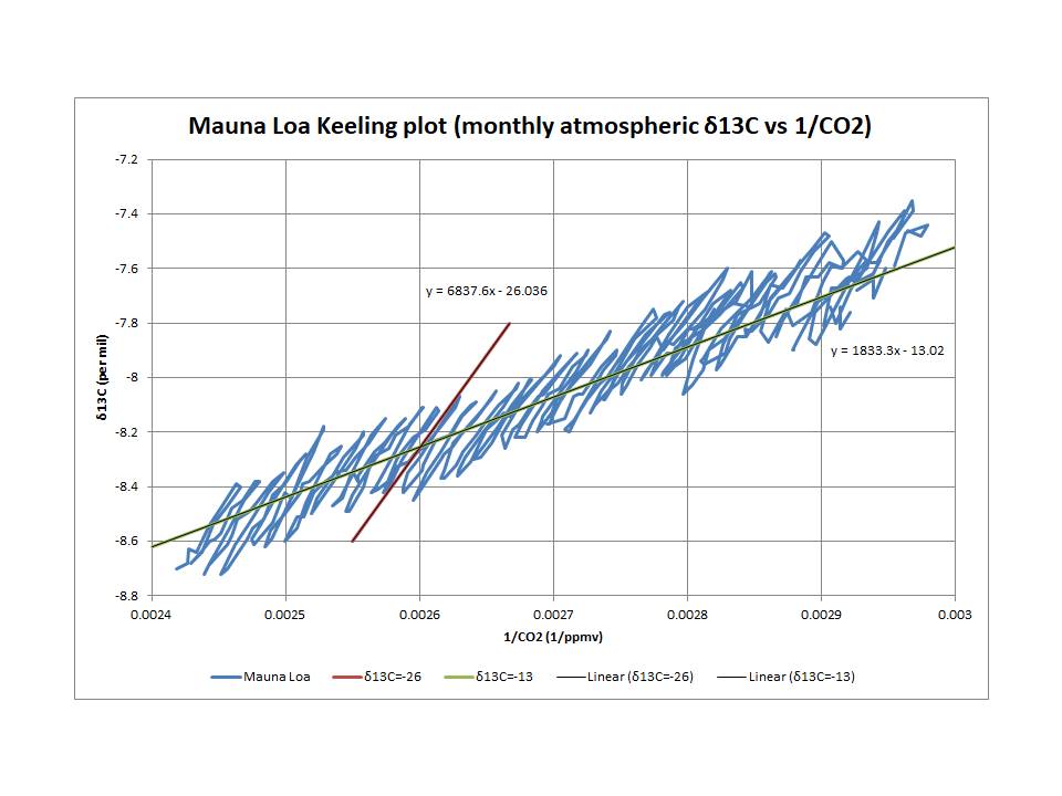
As shown, the annual cycle reflects a roughly -26‰ δ13C, which is consistent with photosynthesis/respiration, while the longer term trend reflects a significantly higher δ13C value of -13‰. This latter trend dominates over the longer term (more than a year) and incorporates δ13C variations due to ENSO and Pinatubo. (As you probably know, the δ13C of fossil fuel burning is estimated to be around -28‰.)
MLO does not measure and record ocean temperatures near shore or at a reasonable distance out. Summers heat up. Winters cool down. The amount of CO2 drawn in the water is a function of partial pressure in air and water and temperature of air and water. Temperature is dominated by water and partial pressure by air. I simplified. The concentration of CO2 in water is not partial pressure, but it has a similar effect.
Clyde, the use of the 12-month-average-change removes the seasonal signal while preserving all the data, and the ERSSTv5 ≥25.6°C 12ma∆ is for the whole ocean, not hemisphere specific.
I claim there are two processes in parallel that make the annual ML cycle work.
The primary one being the result of the annual solar insolation cycle that peaks in the southern hemisphere at the December solstice with help from the perihelion in early January, with it’s cumulative ocean warming effect peaking in March that steadily increases CO2 outgassing until May, after the peak outgassing effect from the SH summer ends and the NH spring CO2 drawdown secondary process begins.
The NH CO2 drawdown is concurrent with the Niño3 region temperature dropping below the 25.6°C outgassing threshold, enabling seasonal Niño3 CO2 sinking. Both mechanisms act to reduce the ML CO2 from it’s annual May peak.
This is reflected in the detrended monthly annual Niño3 and ML data which were used to determine the outgassing temperature threshold.
In the next graphic, the green annual net ML CO2 flux is the difference between the red annual ML rising phase and the light blue annual ML sinking phase timeseries. Assuming the average annual 80.8% ML sink rate vs the annual ML rise rate, the annual man-made portion of the annual ML rising phase in black is also sunk by the same 80.8% amount to the gold-colored line, which is noticeably less than the green annual ML net CO2.
Part of the difference between the net annual ML in green and net annual MME in gold is the outgassing contribution, which is a larger percentage than MME.
If no one recognizes these relationships, their models will predict less future CO2 than nature will actually continue to provide in the event of reduced MME.
Bob, your model seems to neglect some contributions to the annual changes. Most notably, there is no mention of the contribution to the seasonal ramp-up phase from respiration from the roots of dormant trees, particularly the boreal forests in North America and Siberia. These are obviously important because the seasonal CO2 variance increases going from the South Pole to Point Barrow.
The other thing that is important is the bacterial and fungal decomposition of terrestrial vegetative detritus, accompanied by marine photosynthetic die-offs as the sun gets low on the horizon and no longer provides sufficient illumination to sustain the surface populations. As the plankton dies, it immediately starts to decompose, and in shallow water will de-gas rather than dissolve in water as happens at greater depth.
If I remember correctly, Englebeen has claimed that Henry’s Law doesn’t adequately explain the natural CO2 sources, and I believe my remarks above provide reasonable alternative sources to out-gassing from the oceans.
“your model seems to neglect some contributions to the annual changes.”
True, those contributions were not included in my simplified explanation.
“These are obviously important because the seasonal CO2 variance increases going from the South Pole to Point Barrow.”
The spatial variance is due to a larger cold water CO2 sinking surface area of the southern ocean compared to the smaller northern ocean cold sinking surface area.
“Englebeen has claimed that Henry’s Law doesn’t adequately explain the natural CO2 sources”
Englebeen is one who hasn’t recognized the positive contribution from ocean outgassing (the red line in my last image), so his conclusions are wrong.
“By assuming all the increase in atmCO2 is only from man-made emissions”
When manmade emissions are approximately double the atmospheric CO2 increase, nature MUST BE a net CO2 absorber.
This is not a mere assumption
Nature has been a CO2 absorber for billions of years. This is not a new trend.
That naturally absorbed CO2 is currently sequestered as carbon in rocks, shells, oil, gas and coal.
That is also not an assumption
The ocean’s contribution to atmospheric CO2 has been zero for a long time. The oceans are merely absorbing slightly less of the manmade increase in atmospheric CO2 because they are slightly warmer than in the past. Your conclusion is wrong
Annual manmade CO2 emissions = 2x
Annual nature absorption of CO2 = (-1x)
Annual Increase of atmospheric CO2 = 1x
Annual manmade flux 4% of total
Annual Natural flux 96% of total
Because nature cannot tell the difference, basically all man-released CO2 is absorbed into an INCREASING carbon cycle.
Natural warming means there the Natural releases increase, on land and at sea.
They are NOT static. !
BeNasty, you are the dumbest commenter here. I am confient that some leftists pay you for science denying posts that embarrass conservatives.
YOU ARE COMPLETELY IGNORIN ANNUAL NATURAL CO2 absorption that is slightly LARGER than annual natural CO2 emissions.
Over time nature has been a net CO2 absorber.
That’s why atmospheric CO2 was down to 180 ppm just 20,000 years ago, not far above a level that would seriously harm C3 plant growth.
Ignoring the simple fact that natural processes are a major contribution to increased atmospheric CO2 is the same error made by IPCC. Just in the case of oceans a small increase in ocean temperature releases many more times CO2 than anthropogenic CO2 emissions.
Oceans have been absorbing CO2 for over a century, not adding to atmospheric CO2
You are clueless.
That’s stupid. Of course they absorb but they also emit. If you deny that you are ignorant about some basic physical laws.
Although I find Richard‘s insult unacceptable, his argument about nature being a net carbon sink, in particular the biological world is correct. Every carbon atom, that you or your cow expire, must have previously been extracted from the atmosphere via photosynthesis ( https://klima-fakten.net/?page_id=8076&lang=en ).
Regarding the ocean, things are a bit trickier. You both make a correct point. It is true that increasing temperature increases natural emissions, but it is also true that oceans are net sinks. My paper referenced in the first line of this post proposes an elegant explanation, also for the weird phenomenon, why the sink rate described in this post apparently shows no temperature trend at all, despite the fact that global temperature has risen considerably over the last 65 years.
The fact is that natural to anthropogenic CO2 is 20:1 both in terms of emission and absorption. There is no evidence that this ratio has changed to any great extent during modern times and is consistent with the minimal effect of the pandemic on MLO measurements. During this time temperature has increased which has a huge positive impact on ocean emissions and at the same time anthropogenic emissions steadily increased (contrary to Hausfather’s flat anthropogenic emissions for 10 years). Using global values for the past century or so shows that net ocean outgassing (increase in atmospheric CO2 (220) + soil&vegetation (620) – anthropogenic (480)) is about 360 GT C which is not quite a net absorber even though the estimated values are undoubtedly rough.
“world anthropogenic emissions”
“contrary to Hausfather’s US flat anthropogenic emissions for 10 years”
Due to the fact that absorptions are proportional to concentration, even during the time of rising emissions the airborne fraction (concentration growth divided by emissions) reduced from 60% to 50% over the last 64 years. With constant emissions the annual increase of atmospheric CO2 decays exponentially with a time constant of 50 years, as shown in my previous contribution: https://wattsupwiththat.com/2023/03/25/emissions-and-co2-concentration-an-evidence-based-approach/
P.S: The blue graph in Figure 7 also shows how concentration growth declines.
The photosynthetic impact in the oceans is much speed-ed with CO2 levels rising. The bottleneck is Fe.
This in my view explains the lower CO2 levels near the surface.
With populations flattening and fertilizer use rising farm area will peek or even fall these are very positive impacts for the world.
0.3% fall is almost to much for a well fed world.
I like your graph, Bob.
I reached the same conclusion, that temperature preceeds CO2 growth, but I got there by a different route. I watched a video by the late Dr. Murry Salby in which he said there was a corellation between changes in temperature and changes in CO2 growth.
I thought this was interesting so I downloaded the UAH lower troposphere data, calculated the annual average for each year, and plotted some graphs of annual temperature and annual CO2 growth but also change in temperature and change in CO2 growth.
Your use of the sea surface data is going to give better corellations than using atmospheric temperature data but the relationship does show up.
The change in global average temperature and change in global CO2 growth is below. When there is an prolongued or large increase in temperature, there is an increase in CO2 growth. That is an increase in the rate of increase.
More importantly, when there is a decrease in temperature, there is a decrease in the rate of increase. A decrease in CO2 growth. This cannot be the CO2 driving the temperature change since a decrease in the rate of increase is still an increase in CO2 concentration.
An increase in CO2 concentration is supposed to cause an increase in temperature, not a decrease.
Therefore, temperature has to be the independent variable, and CO2 growth the dependent variable.
Something to note is that when calculating the average yearly temperature, the mean centres around the middle of the year. When NOAA calculate the CO2 growth, they average the values for December and January, so that value centres around the end of the year. This puts a 6 month delay in the CO2 growth values.
I have also got quite good corellations using other temperature data. So far I have looked a GISSTemp, NCEI and HadCRUT5. The relationship shows up in all of them.
“Therefore, temperature has to be the independent variable, and CO2 growth the dependent variable.”
Outstanding, and great initiative. It’s definitely an eye-opener.
Thanx for your comment John.
There are a number of studies that find CO2 follows temperature in both the historical and instrumental period. Humlum’s website, climate4u.com, has quite a bit of information.
Oops. I just noticed the left hand y-axis on my graph is incorrectly labelled in that graph.
It should be either dG/dt (Change in growth over time) or dCO2/dt^2 (change in CO2 over time squared.)
One thing your model quite clearly shows is the ability to “turn back the clock” CO2-wise.
If your model is close to the real world (and I do not see why not – seems certainly more real than the Bern outputs to me), once the CO2-hypothesis is proven and there is clear evidence for harm by anthropogenic CO2 (contrary to the current observation of global greening),
mankind has the ability to respond within a decade or two!
Simply reducing the CO2 output by 20% or 40% will reduce the atmospheric CO2 concentration quickly to a level not seen in 50years.. (and this is a relative statement, so it can be done at any future point on that curve, there is absolutely no reason for any panic)
Comment says:”…mankind has the ability to respond within a decade or two!”
There can be no grand response that causes ppm CO2 to decrease without the death of millions. I for one have no stomach for the unnecessary culling of the human race.
That seems right. Overt culling would be bad. Population growth is being intentionally attacked or curtailed, however.
Not sure if I understand this claim you are making here.
How many people died in the USA as a direct consequence of lowering the CO2 emission in the US by about 20% over the last 15 years?
Realistically we should accept something between constant emissions and 1% yearly reduction, depending on the speed of nuclear and PV development.
In both cases we do not expect a catastrophic outcome.
Please explain why we need any reduction in CO2.
We do not need reductions. I am describing what we can realistically expect.
Realistically we should be concerned with our air pollution and not CO2 emissions.
There is zero evidence that increasing atmospheric CO2 has caused harm and strong evidence it has been beneficial.
More so for water pollution and landfills and dumping in the oceans.
Or the growth of Gas and decline of coal. With nuclear obviously solar is a joke in general.
“Simply reducing the CO2 output by 20% or 40% will reduce the atmospheric CO2 concentration quickly to a level not seen in 50years”.
That is a fantasy
Reducing GLOBAL annual CO2 emissions by 20% to 40% would require a similar sized reduction in global GDP.
That’s not going to happen.
175 of 195 nations have no interest in reducing their CO2 emissions.
Also, no climate scientists with sense claims that existing atmospheric CO2 can be removed quickly. You seem to have invented a new theory.
>> That is a fantasy
Because you say so?
>> Reducing GLOBAL annual CO2 emissions by 20% to 40% would require a similar sized reduction in global GDP.
How much did the USA GDP shrink in the last 15 years while the US CO2 emission went down by about 20%?
>> Also, no climate scientists with sense claims that existing atmospheric CO2 can be removed quickly. You seem to have invented a new theory.
Or you dont know what you are talking about! From the article above:
“””How does the Bern Model explain the high yearly absorption rate of more than 6% of the 14C from the bomb tests for 30 years after 1963? “””
Maybe your climate scientists dont know what they are talking about either.
I would start with the claim that there currently is about 30% more CO2 in the atmosphere compared to the presumed equilibrium 200 or so years ago and the oceans temperature and CO2 solubility has not changed significantly for this estimate.
Together with the Revelle factor that means that physical exchange rates between oceans and atmosphere are increased by about about 30%/10 = 3% into the oceans and depressed by about 3% getting CO2 out of the oceans (real world actually shows a two step process as the near surface sea water is close to equilibrium with the atmosphere, but these 6% per year are quite explainable with diffusion and some greening of the planet)
A higher atmospheric partial CO2 pressure of course leads to more removal per year and more global greening.
Maybe your climate scientists should remember some high school science.
Atmospheric CO2 levels are up 50% since 1850 not up 30% in 200 years as you falsely claimed
You can’t even get the most basic climate science fact correct.
story tip
Seeking carbon-free power, Virginia utility considers small nuclear reactors
https://www.nbcwashington.com/news/local/seeking-carbon-free-power-virginia-utility-considers-small-nuclear-reactors/3661076/
What about shell production? Life in the ocean converts CO2 into CaCO3, which is eventually subdued by plate tectonics to produce limestone, which is further reduced by iron to form rock and natural gas.
That‘s definitely part of it. The nice thing about a top down model is that you do not have to deal with each individual contribution. Eventually the results of all individual effects have to be consistent with the top down result of global measurements.
What about Lake Nyos? It shows that CO2 rich sinks of near infinite capacity may exist on the floor of the ocean deep.
Wow.
Science.
Take a look at http;//www.retiredresearcher.wordpress.com/about and click on Nature’s Net-zero.
Thanks, looks very promising
I read only the Conclusion
From the conclusion, I read:
“the fact that since more than 10 years anthropogenic emissions have been approximately constant.”
I looked up manmade CO2 emissions
in billion metric tons
2012 34.94
2022 37.15 (Up +6.2%)
Up 6.2% is slower than the prior decade but
does not fit my definition of approximately constant. If the author can not get a simple fact right, that took one minute for me to look up, then he is an unreliable author.
We don’t need any models to know that humans are adding CO2 to the atmosphere faster than nature is absorbing the extra CO2. The open question is whether that will be a problem in 100 to 200 years if the trend continues.
The growth rate of CO2 emissions may be declining due to Nut Zero in some nations, but there are still a lot of coal power plants being built in other nations. EVs are not having a strong growth rate anymore.
If you take the trouble to actually read the post, you might have noticed that the statement, that emissions have been constant for more than 10 years, is from Zeke Hausfather at CarbonBrief.
So in your wise judgement, Hausfather is an unreliable author. Good to know, I thought he was a sincere scientist, and I took his work seriously.
Why would you include a statement that you believe to be false in your conclusion? With no comment saying that it is false?
That make no sense.
if Nut Zero stops the growth of the annual ris of atmospheric CO2 at +2.5%, the effect will be as follows:
The annual rise rate of CO2 of +2.5 ppm a year will gradually become a smaller annual percentage of total atmospheric CO2
So what?
The atmospheric CO2 will still grow +2.5 ppm a year
So far there is no reduction in the global annual output of CO2 emissions.
Anyone who mentions a 20% to 40% reduction of global annual CO2 emissions is living in a fantasy land and shul be ignored.
it seems that ALL of the inputs to these models are WAG’s and in many cases bad ones … its a chaotic system which by definition CAN’T be modeled with any accuracy … this is simply an intellectual circle j*rk and a waste of brain cells …
Shall we continue to model indiviual molecular interactions on a 25 kilometer grid?
The greatest thing climate models have taught us over the last few decades is how truly ignorant we are.
Congratulations, Joachim Dengler, on a great article!
I have also been analyzing the relationship between CO2 concentrations measured at Mauna Loa since 1959, and global CO2 emissions over the same time period.
I’m not clear where the 2.12 PgC/ppm ratio came from. If this is extrapolated to CO2 by multiplying by the ratio of the molecular weight of CO2 (44.01) to the atomic weight of carbon (12.01), then the ratio is 7.77 Pg CO2 / ppm. Based on an average atmospheric pressure of 101.3 kPa and a molecular weight of dry air of 28.96, I get a ratio of 8.006 Pg CO2 / ppm. But this is only a 3% difference, so that it doesn’t make much difference to the linear model.
In my regression, I used 5-year averages for increases in CO2 concentrations and emission rates, to smooth out some of the variations, resulting in a natural emission rate of 39.92 Pg/yr, and a rate constant of 0.140 Pg/yr-ppm for the natural sink. This would correspond to a = 0.0175 yr^-1 and n = 4.986 ppm/yr in the notation of Joachim Dengler’s article.
I have also seen slightly different estimates for global anthropogenic CO2 emissions, which show that they have continued to increase through 2022, although the rate of increase has slowed considerably since 2012. The latest value I saw was 37.15 Pg/yr CO2 in 2022, which would correspond to 4.64 ppm/yr. It is possible that global CO2 emissions have continued to increase, since it may be difficult to measure CO2 emissions from China, which has shown the most rapid increase in national CO2 emissions since 2000.
If global CO2 emissions leveled out at 37.15 Pg/yr, the linear model would result in an equilibrium concentration of 551 ppm, but it would take over 200 years for the concentration to reach 550 ppm.
The year 2012 (or 2013) definitely seems to be an inflection point. Starting in 2012, the rate of world population growth started to decline, from 89 million/yr to 70 million/yr in 2022, and the CO2 emissions per capita have also decreased steadily since 2012. A continuation of these same trends would lead to a peak in CO2 emissions of about 41 Pg/yr around 2060, with declining emissions thereafter.
A linear model for the natural CO2 sink makes sense from a theoretical point of view. Photosynthesis is a chemical reaction with CO2 as a reactant, so the linear model would assume that its reaction rate is proportional to concentration, for a first-order reaction. Absorption of CO2 into the ocean also depends on Henry’s law, which is also a linear relationship for a given ocean temperature.
Thanks, especially for the plausible reasons, why photosynthesis and ocean absorption/emission are linear processes. I couldn‘t have said it better.
Given the improved productivity of the biosphere, surely accelerating atmospheric CO2 would be the desirable target. China and India are currently doing most of the heavy lifting in this regard.
😂🤣😂
Harold the Organic Chemist Says:
ATTN: EVERYONE!
RE: CARBON DIOXIDE DOES NOT CAUSE WARMING OF AIR!
Using Google, you should search for: “Still Waiting for Greenhouse”.
This is the website of the late John Daly.
From the home page, scroll down to the end of the page, and then click on
“Station Temperature Data”. On the “World Map”, click on “North America”,
and then click on “Pacific”, scroll down and finally click on “Death Valley”.
Shown in the Figure, are plots of the annual seasonal average temperatures
and the annual average temperature. The plots are fairly flat, especially the
annual average temperature. In 1923, the concentration of carbon dioxide was
300 ppm by volume. This is only 0.589 grams of carbon dioxide per cubic meter
of air. By 2001, the concentration of carbon dioxide had increased to 370 ppm
by volume. This is 0.727 grams of carbon dioxide per cubic meter of air.
Based the above data, I have concluded that the increase in carbon dioxide
from 1923 to 2001 in Death Valley did not cause any measurable heating of
the desert air.
At the MLO in Hawaii, the concentration of carbon dioxide is 427 ppm by volume
for March. This is only 0.839 grams of carbon dioxide per cubic meter of air. At
20 deg C, 1 cubic of air has a mass of 1.20 kilograms. This small of amount of
carbon dioxide in air can only heat up such large mass of air by a very small
amount.
Based on the above data and analysis, I have concluded that the claim by the
IPCC that carbon dioxide is the “cause” of the recent “global warming” is a lie.
Since there is only a trace amount of carbon dioxide in air, we need not worry
about it, and we should not be wasting so much time and effort on studies and
investigations of this gas in the air.
P.S.: I am retired organic chemist with a B.Sc.(Hon) and Ph.D.
The IPCC is focused on “human-induced” climate change as dictated by their charter. As a result, they do not include, for example, studies showing that CO2 lags temperature and so cannot be the cause of increased temperature. The lag in my view is the clearest empirical evidence that the AGW hypothesis is nonsense.
“There are three types of sinks that absorb CO2”
I think rain is an overlooked process. Each raindrop scrubs nitrogen and CO2 from the atmosphere on its way to the surface. Depending on surface temperatures the CO2 will either renter the atmosphere or it will come into contact with the surface and remain in fluid within the soil, at which time a variety of chemical and biological processes will consume it.
The dwell time on average of an atmospheric CO2 molecule on this planet, is one (1) year.
The amount of CO2 the oceans will hold is based on temperature and the density of ions such as Magnesium and Calcium Ions that mineralize CO2 on contact instantly. This is a hostile planet for CO2, its barely hanging on, that is why it is a rare gas.
The pH of the ocean is about 8.1 to 8.2. When CO2 enters the ocean, a portion of it is
converted mostly to bicarbonate and some to carbonate anions. This is a buffer that helps maintains the pH in the 8.1 to 8.2 range.
A large portion of the CO2 is fixed by phytoplankton and aquatic plants via photosynthesis as evidenced by the abundance of plants and animals which feed on these. Magnesium and calcium do not react with CO2.
On land another large amount of CO2 is fixed by plants via photosynthesis.
At the MLO in Hawaii, the concentration of CO2 in air is 427 by volume. This is only 0.839 grams of CO2 per cubic meter of air. This low amount of CO2 in air can not
cause global warming.
Hi Harold.
You said “The pH of the ocean is about 8.1 to 8.2.”
You are not wrong but it’s worse than that.
On page 293 of the IPCC Fifth Assessment Report (AR5) it says that “The mean pH (total scale) of surface waters ranges between 7.8 and 8.4 in the open ocean, so the ocean remains mildly basic (pH > 7)”
The normal range of oceanic pH is much larger than the so called effect of increasing CO2.
I like to use the official IPCC statements to show that the claims do not make sense.
Hi LT3
I agree that rain is an overlooked process.
Check out https://retiredresearcher.com/
This site has some very good analysis of the CO2 problem.