UAH Global Temperature Update for April, 2024: +1.05 deg. C

From Dr Roy Spencer’s Global Warming Blog

Roy W. Spencer, Ph. D.

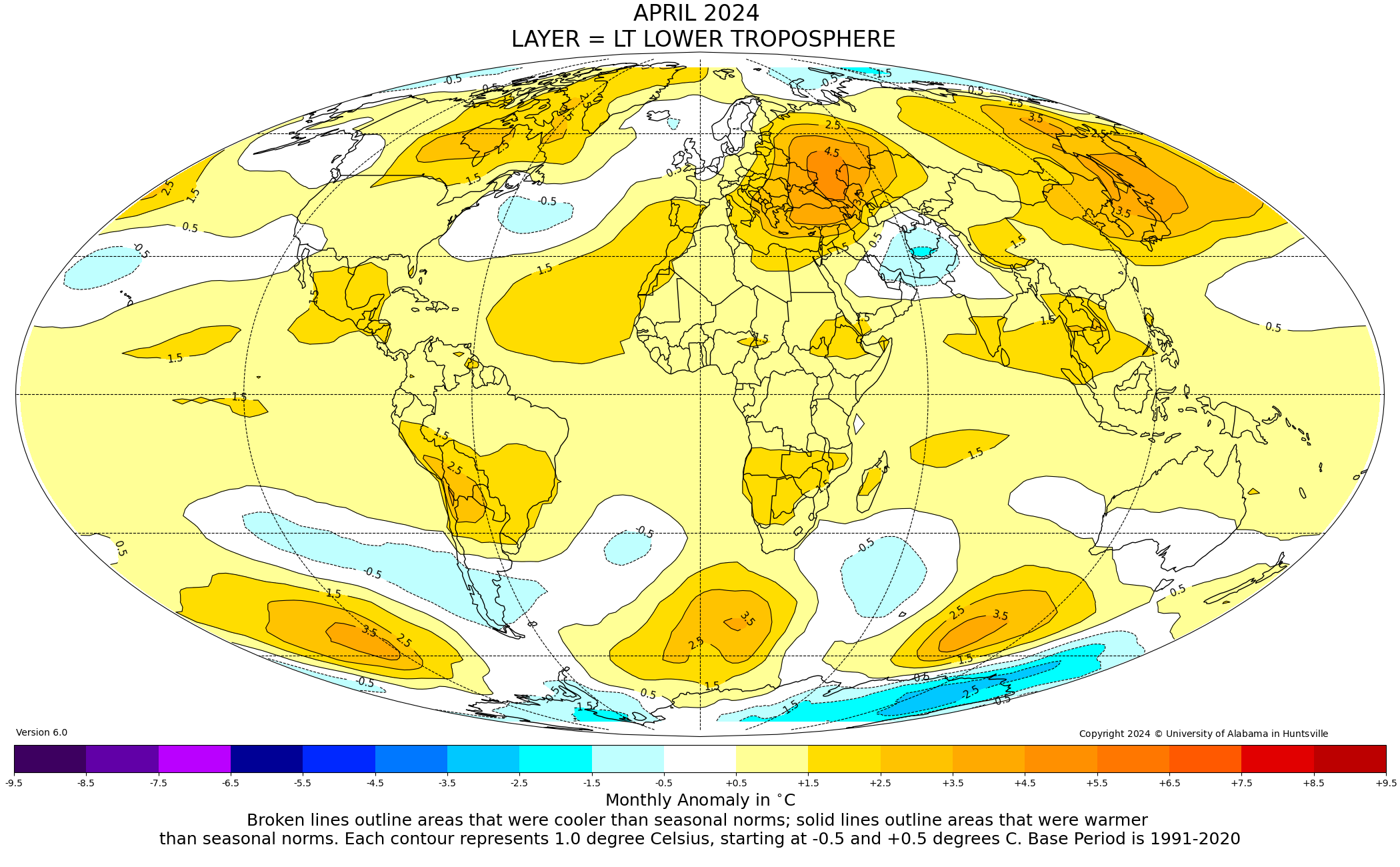
The Version 6 global average lower tropospheric temperature (LT) anomaly for April, 2024 was +1.05 deg. C departure from the 1991-2020 mean, up from the March, 2024 anomaly of +0.95 deg. C, and setting a new high monthly anomaly record for the 1979-2024 satellite period.

The linear warming trend since January, 1979 remains at +0.15 C/decade (+0.13 C/decade over the global-averaged oceans, and +0.20 C/decade over global-averaged land).

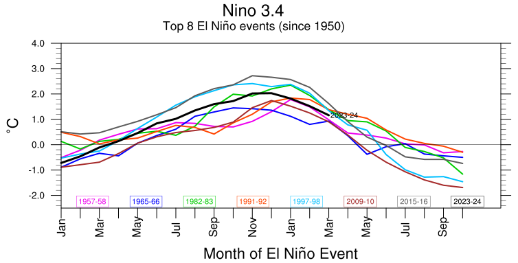
It should be noted that the CDAS surface temperature anomaly has been falling in recent months (+0.71, +0.60, +0.53, +0.52 deg. C over the last four months), while the satellite deep-layer atmospheric temperature has been rising. This is usually an indication of extra heat being lost by the surface to the deep-troposphere through convection, and is what is expected due to the waning El Nino event. I suspect next month’s tropospheric temperature will fall as a result.

The following table lists various regional LT departures from the 30-year (1991-2020) average for the last 16 months (record highs are in red):

YEARMOGLOBENHEM.SHEM.TROPICUSA48ARCTICAUST
2023Jan-0.04+0.05-0.13-0.38+0.12-0.12-0.50
2023Feb+0.09+0.17+0.00-0.10+0.68-0.24-0.11
2023Mar+0.20+0.24+0.17-0.13-1.43+0.17+0.40
2023Apr+0.18+0.11+0.26-0.03-0.37+0.53+0.21
2023May+0.37+0.30+0.44+0.40+0.57+0.66-0.09
2023June+0.38+0.47+0.29+0.55-0.35+0.45+0.07
2023July+0.64+0.73+0.56+0.88+0.53+0.91+1.44
2023Aug+0.70+0.88+0.51+0.86+0.94+1.54+1.25
2023Sep+0.90+0.94+0.86+0.93+0.40+1.13+1.17
2023Oct+0.93+1.02+0.83+1.00+0.99+0.92+0.63
2023Nov+0.91+1.01+0.82+1.03+0.65+1.16+0.42
2023Dec+0.83+0.93+0.73+1.08+1.26+0.26+0.85
2024Jan+0.86+1.06+0.66+1.27-0.05+0.40+1.18
2024Feb+0.93+1.03+0.83+1.24+1.36+0.88+1.07
2024Mar+0.95+1.02+0.88+1.34+0.23+1.10+1.29
2024Apr+1.05+1.24+0.85+1.26+1.02+0.98+0.48

The full UAH Global Temperature Report, along with the LT global gridpoint anomaly image for April, 2024, and a more detailed analysis by John Christy, should be available within the next several days here.

The monthly anomalies for various regions for the four deep layers we monitor from satellites will be available in the next several days:

Lower Troposphere:

http://vortex.nsstc.uah.edu/data/msu/v6.0/tlt/uahncdc_lt_6.0.txt

Mid-Troposphere:

http://vortex.nsstc.uah.edu/data/msu/v6.0/tmt/uahncdc_mt_6.0.txt

Tropopause:

http://vortex.nsstc.uah.edu/data/msu/v6.0/ttp/uahncdc_tp_6.0.txt

Lower Stratosphere:

http://vortex.nsstc.uah.edu/data/msu/v6.0/tls/uahncdc_ls_6.0.txt

4.9 12 votes
Article Rating
Subscribe
Notify of
668 Comments
Oldest
Newest Most Voted
Inline Feedbacks
View all comments
CD in Wisconsin
May 4, 2024 2:07 pm

“…… and setting a new high monthly anomaly record for the 1979-2024 satellite period.”

This will surely send the alarmists into hysteria mode. “See, we told ya!”

Rich Davis
Reply to  CD in Wisconsin
May 4, 2024 2:30 pm

If the earth were going through a multi-decadal slight cooling trend, I wonder if the commie parasites would be saying that we’ve got to stop burning fossil fuels to save The Planet ™? Oh wait they did that already in the mid 70s.

Reply to  Rich Davis
May 5, 2024 12:27 pm

I remember because I was there. In the winter of 77 it seemed infinitely plausible, while I was standing in six feet plus of snow with drifts up to the power wires on the telephone poles, but like all their predictions the apocalypse failed to appear. I quit listening long ago🤷‍♂️🤔

Bryan A
Reply to  CD in Wisconsin
May 4, 2024 6:49 pm

User…
User…
Here ya go!!!

Bryan A
Reply to  Bryan A
May 4, 2024 11:15 pm

Hmmm
9+ hours into the conversation and who’s missing?
The one constant complainer that a post was missing
Myusername

Stokes is here (but Nick wasn’t complaining)
Walton is here (but Isaac wasn’t complaining)
Bellman is here (but Bellman wasn’t complaining)
TheFinalNail is here too (but TFN wasn’t complaining)

The missing person in this debate is Myusername who was fervently complaining in an unrelated post that this particular post was missing because the skeptical side found the data to be inconvenient.

User…
User…

Reply to  Bryan A
May 5, 2024 7:33 pm

Love Ferris Username’s day off, great fun.

May 4, 2024 2:16 pm

It’s an El Niño year. El Niño years are always hotter and break trend.


El-Nino-years
Nick Stokes
Reply to  John Reistroffer
May 4, 2024 2:33 pm

Yes. But they are now also hotter than earlier El Niño years . As your plot shows, this whopper is not a particularly strong El Niño.

Rich Davis
Reply to  Nick Stokes
May 4, 2024 2:42 pm

Yawn, hotter!
6°C this morning in Northern Connecticut.
I’ll happily take about 20° warmer thank you very much.

Reply to  Nick Stokes
May 4, 2024 2:45 pm

” not a particularly strong El Niño.”

Enso index is only a small part of the El Nino region.. a good indicator of “when” but not of how wide-spread.

The amount of energy released has been enormous.

Enough to heat the whole atmosphere in only a couple of months and hold it there for several more, spreading it widely.

Note however, that the Tropics, where all this energy emanates from, seems to have dropped a bit.

Indian ocean dipole is also in a very warm phase.

Thomas
Reply to  bnice2000
May 4, 2024 3:30 pm

This is usually an indication of extra heat being lost by the surface to the deep-troposphere through convection, and is what is expected due to the waning El Nino event. I suspect next month’s tropospheric temperature will fall as a result.

This is why global average temperature tells us nothing of value about whether heat was added to, or removed from, the ocean/atmosphere system. In an El Niño hot water that was buried deep in the Pacific warm pool sloshes back across the Pacific and is exposed to the atmosphere, so the troposphere warms as the ocean cools. Overall, the system cools during an El Niño. The troposphere warms as the heat travels from the warm pool to deep space but the overall system cools.

The fact that the key metric for “global warming” (average tropospheric temperature) goes up when the earth system is cooling is a pretty good clue that the metric is not fit for purpose. There are also other reasons that it isn’t fit. Like the fact that temperature is not a measure of the heat content of atmospheric air.

To borrow from Jonny Cochran, “If the metric don’t fit, it ain’t legit.”

Chris Hanley
Reply to  Nick Stokes
May 4, 2024 4:45 pm
bdgwx
Reply to  Chris Hanley
May 4, 2024 7:18 pm

It’s not perfect, but the relationship looks decent to me.

comment image

Reply to  bdgwx
May 4, 2024 7:26 pm

Your stupid little conjecture driven model, yet again.

Hilarious! And not remotely science.

resiurkigam
Reply to  bdgwx
May 4, 2024 7:29 pm

What is your forecast for July 2028?

bdgwx
Reply to  resiurkigam
May 4, 2024 7:52 pm

I don’t have one.

resiurkigam
Reply to  bdgwx
May 4, 2024 8:44 pm

What utility does a model provide without the ability to forecast?

Bryan A
Reply to  resiurkigam
May 4, 2024 10:37 pm

You can dress them up and sell their pictures to the media for a prophet

Keith Van
Reply to  Bryan A
May 5, 2024 12:24 pm

If we could sell them for a real prophet then he could tell us what the temperatures will be decades from now. But for now, they will just settle for obscene profits. 😀

Tom Johnson
Reply to  resiurkigam
May 5, 2024 4:48 am

A useful model can provide insight to the process being modeled, and insight can provide better understanding of the science involved. (Remember the George Box idiom “All models are inaccurate, some are useful”) Models rarely, if ever, provide precisely accurate forecasts. In general, the higher the complexity, the higher the inaccuracy. Few models are as complex as climate models.

bdgwx
Reply to  resiurkigam
May 5, 2024 6:20 am

Assuming we define “prediction” as a statement of an outcome given a set of conditions and “forecast” is a subset of a “prediction” whose statement of an outcome involves the future then my answer is that the ability to forecast is not necessary to make a prediction. And it’s only prediction that is a trait that is necessary for a model to be useful. An example…PV=nRT is a model without a time dimension. But it still makes predictions and is useful in that respect despite its inability to forecast (on its own). I often see the words diagnostic and prognostic used in literature to describe models that only make predictions vs those that make forecasts.

The model I show above is classified as diagnostic not unlike the PV=nRT model. I do show a forecast out to 2024/10 but that’s only because I use a separate prognostic model for the ENSO forecast in the future and then use that as input.

Reply to  bdgwx
May 7, 2024 6:53 pm

An important distinction for PV=nRT versus climate models is that it is correct for any time, given that one knows two of the three variables accurately for the time of interest. Thus, if one can predict two of the variables accurately for some time in the future, the third variable can similarly be predicted with the same accuracy. Climate models are so poor that they are unreliable for any time.

bdgwx
Reply to  Clyde Spencer
May 9, 2024 6:12 am

CS: An important distinction for PV=nRT versus climate models is that it is correct for any time

Nah. It’s correct only for ideal gases. No gas is actually ideal so applying the IGL is wrong most of the time. But, it’s still useful because it is close enough most of the time. F=ma is another example of this concept. We know that it is wrong. But, it’s still useful because it is close enough most of the time.

My point still remains. A model only needs to make predictions to be useful. It does not need to make forecasts.

Reply to  bdgwx
May 9, 2024 6:37 am

Don’t make strawman arguments. The Ideal Gas Law is correct for an ideal gas ALL the time. F = ma is correct for non-relatistic calculations. The real problem is not the formula but measurement uncertainty. It is hard to measure temps to the micro-kelvin or mass to the micro-gram or micro-moles of a gas. The uncertainty in measurement leads to the great unknown!

Reply to  bdgwx
May 8, 2024 1:00 pm

You just made a strawman argument. PV = nRT is the Ideal Gas Law. It is a law that accurately relates the components specified. Time is not part of the relationship, therefore the strawman.

If you want to include time you could develop a gradient with a time factor such as with Temperature, then integrate it to find how one of the components change over that time while holding the others constant.

Many here seem to think a time series is a tool that can be used to predict CAGW. Believe me, if that was the case everyone would be rich from investing based on a stock’s time series and simple regressions.

Reply to  bdgwx
May 4, 2024 8:03 pm

Where is the the more or less monotonic increase in the atmospheric CO2 concentration. that you responded to, in your graph?

bdgwx
Reply to  philincalifornia
May 4, 2024 8:22 pm

It’s the 1.8 * log2(CO2lag1/CO2initial) term.

Chris Hanley
Reply to  bdgwx
May 4, 2024 9:07 pm

Here are similar plots using HadCRUT and Mauna Loa, it looks to me that the rate of change in CO2 lags the rate of change in temperature.

bdgwx
Reply to  Chris Hanley
May 5, 2024 7:58 am

It’s not similar though. That graph is showing changes in temperature and CO2 over a 1 year period and not the actual temperature and CO2 values themselves. Regardless you can see that the blue and red plots (temperature) are flat while the green plot (CO2) is going up so while there is a relationship between temperature changes and CO2 changes on short time scales as a result of natures ability to buffer carbon decreases/increases as temperature increases/decreases there is no relationship between temperature changes and CO2 changes on long time scales. And again…it’s still a presentation of the changes in the quantities and not the quantities themselves and is very different from the first graph you posted.

bdgwx
Reply to  Chris Hanley
May 6, 2024 7:53 am

I should add that my discussion here is in response to the claim that there is no relationship between CO2 and UAH temperatures. As I show in the model above there is clearly a relationship. The model (by itself) is not proof that CO2 or any of the 4 factors necessarily modulate the temperature; we need extra information for that. But it is proof that there is a relationship. That is what I was addressing with my comments to you.

Reply to  bdgwx
May 6, 2024 1:26 pm

‘The model (by itself) is not proof that CO2 or any of the 4 factors necessarily modulate the temperature; we need extra information for that.’

Neither proof nor evidence.

bdgwx
Reply to  Frank from NoVA
May 6, 2024 3:47 pm

It’s definitely evidence that falsifies the hypothesis that there is no relationship between CO2 and temperature. It’s not, however, evidence that CO2 or the other 4 factors are causes of temperatures. For that you need a different kind of evidence. But that’s not the scope of my posts here. The scope of my posts here is to falsify Chris Hanley’s hypothesis.

Bryan A
Reply to  Nick Stokes
May 4, 2024 6:52 pm

Not particularly strong???
An anomaly of 2.05°C in the Niño 3.4 region makes it the 4th strongest El Niño on record. That’s extremely strong, almost unprecedented.

Izaak Walton
Reply to  Bryan A
May 4, 2024 7:25 pm

So if the 4th strongest El Nino counts as “almost unprecedented” how would you describe 10 months of record high temperatures?

Bryan A
Reply to  Izaak Walton
May 4, 2024 10:38 pm

Expected!

Reply to  Izaak Walton
May 5, 2024 1:33 am

Where are these record high temperatures? Certainly not in Northwest Europe, where I live. It has been remarkably cold in Belgium and the UK this year.

Reply to  Graemethecat
May 5, 2024 4:14 am

No record high temperatures here in the central U.S.

Richard Barraclough
Reply to  Graemethecat
May 5, 2024 10:34 am

Cold in the UK?

The Central England Temperature for January to April has been the second highest in the 364 years of records.

Reply to  Richard Barraclough
May 6, 2024 5:48 am

Why is it so damned cold then?

Reply to  Izaak Walton
May 5, 2024 8:03 am

If you are referring to the surface temperature record, I would describe it as poor data skewed by urban heat effects.

bdgwx
Reply to  Mark Whitney
May 5, 2024 8:41 am

He’s referring to the UAH dataset. But even at the surface Dr. Spencer’s analysis showed that UHI bumps the global average temperature by around 0.03 C. It’s important to point out that this is a real effect so its inclusion isn’t skewing anything.

Reply to  Bryan A
May 7, 2024 6:58 pm

The duration of the temperature peak of the “not particularly strong” El Niño is also anomalously long.

resiurkigam
May 4, 2024 2:19 pm

Nothing says the planet can’t abruptly descend into near-glacial conditions at any point in the future.

Reply to  resiurkigam
May 5, 2024 7:49 am

Indeed, we have no idea about short-duration changes preceding a glacial advance. A series of strong positive ENSO events could be a sign of planetary thermal changes leading to a glacial episode. CO2 may have no real influence at all.

resiurkigam
Reply to  Mark Whitney
May 5, 2024 8:51 am

Mark Whitney,

Thanks for the reply. I’ve been reading up on an event that took place ~11,000 – 12,000 years ago. Proxies tell us that there was a sharp cooling of 4-10°C over the span of just a couple of decades. If the processes that shaped this event started happening today, even older people would witness Little Ice Age conditions, at least.

I am cautious when it comes to interpreting the conclusions of proxies, regardless of whether it comes from skeptics or enthusiasts. But anything can happen is the main point.

This type of event would pose a real challenge for life on Earth, including humanity since it would be really hard to foresee and prepare for. We should be grateful to live in the climate we have today.

comment image

May 4, 2024 2:26 pm

This is the warmest April by 0.43°C. The previous record was set in 1998, but statistically tied with 2016.

 1 2024 1.05
 2 1998 0.62
 3 2016 0.61
 4 2019 0.33
 5 2020 0.27
 6 2022 0.27
 7 2005 0.20
 8 2010 0.20
 9 2017 0.19
10 2023 0.18

This makes 10 record months in a row.

The next couple of months will be interesting for records. May and June’s records were both set in 1998, 0.52C and 0.44C. If those records hold, it will mean a record drop in anomalies over the next two months – so either way records will break.

Reply to  Bellman
May 4, 2024 2:29 pm

Here’s a side by side comparison of the three main El Niño events in the UAH data set.

comment image

It’s interesting how much temperatures have increased since the start of the year, when it looked as if the peak had already been reached last October.

Rich Davis
Reply to  Bellman
May 4, 2024 2:38 pm

Isn’t it so exciting?

Warmer is better and more CO2 means more life.

Reply to  Bellman
May 4, 2024 2:48 pm

Yep, It has been a particularly strong and prolonged El Nino event.

Huge amounts of energy released,

Started early and just keeps going.

Nobody in their right mind could possibly blame anything humans have done..

….and in fact no-one has been able to show any human causation whatsoever.

Reply to  bnice2000
May 4, 2024 5:29 pm

Yep, It has been a particularly strong and prolonged El Nino event.

You keep asserting that, but never give any evidence. Most indicators suggest this has neither been particularly strong or prolonged, compared to 1998 and 2016.

comment image

https://psl.noaa.gov/enso/dashboard.html

Huge amounts of energy released,

and why do you think there was more energy to release?

Reply to  Bellman
May 4, 2024 5:37 pm

The evidence is in the response of the atmosphere which you have pointed out several time yourself.

The Nino 3.4 area is a tiny indicator of “when” there is an El Nino.

… and does not indicate how wide-spread it is.

Denial of your own data and own graphs.. That is a pretty stupid thing to do.

Noted that you, yet again, ducked the issue of human causality.

Why do you keep doing that, I wonder.. 😉

Reply to  bnice2000
May 4, 2024 7:34 pm

The Nino 3.4 area is a tiny indicator of “when” there is an El Nino.

I gave you a link to a number of different indicators. Apart from region 4, I couldn’t find any suggesting this El Niño is a strong as 98 or 16, or any indication that it is more prolonged.

The evidence is in the response of the atmosphere which you have pointed out several time yourself.

You keep going round in circles. You claim the record temperatures are caused by the strength of the El Niño, then claim that the strength of the El Niño is proven by the record temperatures.

Noted that you, yet again, ducked the issue of human causality.

This is your own monomania. My argument above has nothing to do with whats casing the warming.

But I keep giving you “evidence” of a link between CO2 and temperature – you just reject it. The fact that there is a statistically significant correlation between CO2 and global temperature is evidence.

If you want more evidence you will have to ask people who understand it more than me. I’m just interested in pointing out what the data says, regardless of what it means.

Reply to  Bellman
May 4, 2024 7:46 pm

Here for example is a somewhat out out of date linear fit for the HadCRUT data set, based on just CO2, ENSO conditions and the AMO. Not perfect, but it captures the main raise in temperature.

TSPauseHAD08
Reply to  Bellman
May 4, 2024 7:51 pm

The red line is the predicted temperature based on the various independent variables. This is trained on the data in green, that is up to just before the pause.

Here’s the same, but I took CO2 out of the equation.

The point is non of this proves CO2 caused the warming, but you do need something to explain the warming trend – and I doubt it’s the price of stamps.

.

TSPauseHAD09
leefor
Reply to  Bellman
May 4, 2024 8:03 pm

You mean like sunlight warming the oceans? Less cloud cover? 😉

Bryan A
Reply to  leefor
May 4, 2024 10:41 pm

Not to mention spurious adjustments to temperature datasets
Both recent (upwards) and historic (downwards)

Reply to  Bryan A
May 5, 2024 4:20 am

Yeah, I think that explains the warming trend.

The warming trend exists only in the computers of climate alarmists.

Richard M
Reply to  leefor
May 5, 2024 5:40 am

Yup, last I looked there’s been about a 1% increase in solar energy reaching the surface since the 2022 Hunga Tonga eruption. That’s on top of a 1.5% increase over the first two decades of the 21st century. Most of this due to cloud reductions.

It’s been added to the El Nino warming over the past year.

Reply to  Bellman
May 5, 2024 11:18 am

Again, these are not normalized to a similar starting point. In January, normalize them to start at 0.0 deg C. That will show that 2023-24 is one of the strongest and reduce 2016 El Niño.

bdgwx
Reply to  Renee
May 5, 2024 12:04 pm

The graph Bellman posted is already normalized at 0 since it is using ONI. The 2023/4 El Nino peaked at 2.0. 1997/8 peaked at 2.4. 2015/6 peaked at 2.6. 1997/8 and 2015/6 were stronger than 2023/4.

Reply to  Renee
May 5, 2024 12:27 pm

You have hit a point that I have fallen into also. The assumption is that ΔT’s can be averaged with no worries or effects statistically really makes little sense. Once aversged you have no way to determine what the global baseline actually is. A global anomaly one month might come out +1.5°C @ 50° and the next month be 2.0°C @ 47°C.

The assumption is that if the baselines of individual stations are always the same then the GAT baseline is always the same. But that ignores the various “weighting” that occurs with varying values at different stations.

Reply to  Renee
May 5, 2024 1:37 pm

I’ve no idea what point you think you are making.

The ENSO index I showed was not my graph, it’s NOAA’s own data. They page I linked to shows a number of ways in which the strength of an El Niño can be assessed. It’s strength is the value of an index, not the amount it climbed from some arbitrary point.

bdgwx
Reply to  Bellman
May 4, 2024 2:50 pm

It’s looking more likely that the UAH response to this El Nino cycle may behave inline with the typical 4-5 month lag behind ONI afterall.

Reply to  Bellman
May 4, 2024 2:52 pm

And the cause is Man and not Natural?
After “The Claim” does not mean because of “The Claim”.

Reply to  Gunga Din
May 4, 2024 2:59 pm

Would you deprive Man of reliable energy to be prepared for the next “ice Age” or the next … what did they call the last “Warm Age”?
Maybe they don’t believe there ever was a “Warm Age”?
(“One too many hits with the Hockey Stick!”)

Reply to  Bellman
May 4, 2024 3:07 pm

For a comparison of the El Niño years, shouldn’t you normalize the beginning of them to start at zero? That would make this one more comparable to the 1997/98 years.

Reply to  Renee
May 4, 2024 4:37 pm

Rather than that, I can remove the linear trend across the UAH data.

comment image

The peak of 2024 is now much closer to that of 1998, though it still started earlier, and ’98 was stronger than 2016.

This illustrates the point, that there has been a warming trend, which means successive El Niños are working from a higher base.

Reply to  Bellman
May 4, 2024 5:44 pm

Again, the Nino3.4 area is an indicator .

It does not and can not tell you how wide-spread the event is or how much energy is released.

All you have to do is look at the atmospheric response.

Started earlier, warming for several months and much more prolonged.

That is according to your own graph. !!

Why the continued idiotic denial of what you yourself has posted. Just dumb !!

Reply to  bnice2000
May 4, 2024 7:42 pm

He seems oblivious to the obvious that the huge warming spikes occurs when there is a significant El-Nino ongoing, the blindness is simply amazing!

bdgwx
Reply to  Sunsettommy
May 4, 2024 8:25 pm

Bellman is aware of ENSO and even factors it into his analysis. See an example here.

Reply to  Sunsettommy
May 5, 2024 5:12 pm

I specifically said it’s warming in response to an El Niño.

Here’s a side by side comparison of the three main El Niño events in the UAH data set.

I really wish WUWT had better threading. Nobody seems capable of following the thread to see how it started.

0perator
Reply to  Bellman
May 4, 2024 4:03 pm

Wow. Spring was so much warmer than winter. Amazing.

Reply to  0perator
May 4, 2024 4:20 pm

They’re anomalies.

Reply to  Bellman
May 5, 2024 8:55 am

Isn’t everything an anomaly?

Reply to  0perator
May 5, 2024 8:55 am

Not in Britain, the last few weeks were reminiscent of February rather than mid spring.

Richard Barraclough
Reply to  JohnC
May 5, 2024 10:55 am

The second half of April, according to the Central England Temperature series, was just below the long-term average, but what made it feel colder was that the first half of April was more than 3 degrees warmer.

Reply to  JohnC
May 5, 2024 1:48 pm

Only becasue this February was so warm.

comment image

Reply to  Bellman
May 5, 2024 12:26 am

Can you include solar activity on your graph? Can you include ultraviolet irradiation levels from the sun?
As sure as eggs is eggs, taking a single phenomenon out of a complex system can be used to prove anything. Even the BBC now includes El Niño in its reports. Also, water will release carbon dioxide into the atmosphere as it warms.

Grumpy Git UK
Reply to  Bellman
May 5, 2024 6:36 am

As you are so convinced that CO2 controls the temperature perhaps you can explain to everyone how the global temperature dropped from around 25C down to 11C while CO2 was at 4000ppm and then went back up to 25C when CO2 was still at 3000ppm and went from 11C to 25C while CO2 was at 1500ppm 200million years later?

Thomas
Reply to  Bellman
May 4, 2024 3:43 pm

To put it in perspective, if all the warming shown in the 45 year UAH global temperature record were to occur in the place where you are situated as you read this sentence, you probably wouldn’t even notice that it happened.

bdgwx
Reply to  Thomas
May 4, 2024 7:10 pm

You probably didn’t mean it this way, but I thought it would be fun to calculate the result if the energy which caused the warming were hypothetically focused onto a single 1 km2 column of atmosphere where you are situated. UAH shows about 0.50 C of warming in the TMT layer. It’s a bulk atmosphere measurement in the troposphere which has a mass of roughly 3.8e18 kg and specific heat capacity of 1 kj/kg.C. That’s about 1.9e18 kj of energy. Focus that 1 km2 column of atmosphere in the place you are situated and it would cause a temperature of 1 kg.C.kj-1 * 1.9e18 kj / (3.8e18 kg / 510e6 km2 * 1 km2) = 255e6 K. You would dissociate into a plasma instantly and be completely unaware that it happened. So yeah, under that scenario you wouldn’t even notice.

Of course you probably were thinking your place warmed by 0.65 C (what UAH shows for the TLT layer). Given a laboratory grade thermometer with a low enough uncertainty and you’d almost certainly notice. I suspect you actually meant that you’d use the good old fashioned skin test though which I wholeheartedly agree would go unnoticed. I can’t speak for everyone, but my own “skin thermometer” has a rather large uncertainty of several degrees C.

Reply to  Bellman
May 6, 2024 7:17 am

As people keep asking where records are being set, here’s a graph showing exactly which grid cells were a record for each specific month. This only goes up to March 2024, as we are still waiting for the April update.

It’s clear that the tropics are the most consistent at setting records. This might reflect the fact that this has been the are with the greatest warming. But it might also be because the tropics have a lot less variability.

20240506wuwt2
Reply to  Bellman
May 6, 2024 7:27 am

This graph shows the number of monthly records set in the past year.

It again shows how prolific the tropics have been at setting records. Some places have had a record month for most of the year. In contrast the central band of the USA has managed to avoid any monthly record.

20240506wuwt1
Reply to  Bellman
May 7, 2024 7:47 pm

In case anyone’s actually interested, the map for April has now been published

comment image

Eastern Europe and Western Russia seem to be the biggest hot spot, along with Japan. And the section of South America that seems to have been above average for ages, is still well above average.

All of the tropics still warm, but it does look like the ENSO region is cooling down a bit.

Rich Davis
May 4, 2024 2:33 pm

This is the Rusty Nail’s favorite topic, where is that bot boy?

Reply to  Rich Davis
May 4, 2024 3:01 pm

Possibly still hunting for some human causation for this El Nino… and not finding any. 😉

Does this El Nino give GW… yes… for a short period…maybe another small up-step as a result

AGW… NOPE !!

May 4, 2024 2:50 pm

Tonga has been a distinct anomaly since Jan ’22 thrusting 40+ trillion gallons of water vapor into the greenhouse system.

Nick Stokes
Reply to  John Shewchuk
May 4, 2024 2:56 pm

It did it just once, in Jan ’22.
This is April ’24

Reply to  Nick Stokes
May 4, 2024 3:05 pm

Comment was expected. Several studies have shown multiple, oscillating effects of terrestrial eruptions (see image) … however, we have no modern-day record of a large submarine eruption (like Tonga) — therefore we are still watching & learning.

Volcanoes
Reply to  John Shewchuk
May 5, 2024 4:27 am

Yeah, what unprecedented event occurred in the Earth’s atmosphere recently?

Still watching and learning about underwater volcanic eruptions into the statosphere.

It looks like last month’s high temperature just about equals the 1934 temperature in the United States. Hansen said 1934 was the hottest year in the U.S., and was 0.5C warmer than 1998.

Reply to  Nick Stokes
May 4, 2024 6:08 pm

OMG, Nick thinks that a volcano that spewed water vapour far into the atmosphere, didn’t also heat the ocean.

That is just hilarious.!

Milo
Reply to  Nick Stokes
May 4, 2024 8:39 pm

Most of the mass of injecte water is still in the stratosphere.

Richard M
Reply to  Milo
May 5, 2024 6:15 am

Exactly, it is too light to fall out. It will eventually react with other things lowering the concentration but no one knows how long it will take.

Initially there were also cooling gases such as SO2, but they did fall out and that cooling effect has almost completely ended. That’s probably why we didn’t see an immediate warming effect.

https://acd-ext.gsfc.nasa.gov/Data_services/met/qbo/h2o_MLS_vLAT_qbo_75S-75N_10hPa.pdf

Milo
Reply to  Richard M
May 5, 2024 12:45 pm

That’s one big reason, for sure.

You’re also right that water is lighter than air, unlike CO2. However, its molecules can clump together to form droplets, as in fog or clouds, or ice crystals, as in cold clouds.

Raining or snowing out of the stratosphere is not trivial, though.

Phil.
Reply to  Milo
May 6, 2024 12:46 pm

Based on the phase diagram of water it’s not going to form droplets in the stratosphere

Bryan A
Reply to  Nick Stokes
May 5, 2024 7:23 am

And most of that upper atmospheric water vapor is still in the column
comment image

sherro01
Reply to  Bryan A
May 5, 2024 3:36 pm

Bryan A,
Please try to start the Y axis at zero when the data cover a range not far from zero. Even if you copied the art work of another author, there is no restriction on a small modification to show better practice with a note saying why you did it. Not a major gripe, I’m trying to be helpful. Geoff S

Reply to  sherro01
May 5, 2024 5:42 pm

Disagree. Brian A wanted to highlight the increase in [water vapor] from the eruption, and what we know now about it’s return. I think he did so.

Now, let’s review the dat based comments here on it’s actual impact…

bdgwx
Reply to  John Shewchuk
May 4, 2024 3:01 pm

If the belief is that 150 MtH2O can cause that much warming then it seems it would be cavalier to dismiss the effect of the 90000 MtCO2 that got thrusted into the greenhouse system since Jan ’22.

Reply to  bdgwx
May 4, 2024 6:24 pm

[Assuming those figures are accurate] The CO2 IR bands are pretty much saturated already. For H2O it isn’t, and absorbs across a much larger length of the spectrum. Water vapor can also form heat-trapping cirrus clouds. The H2O will remain up in the stratosphere for a while. Carbon dioxide emitted into the troposphere can be sequestered quickly by the biosphere. Is that 90,000 Mt gross or net?

Richard M
Reply to  johnesm
May 5, 2024 6:18 am

CO2 is also a well mixed gas. This turns out to be very important part of the science. It keeps the energy flowing up through the atmosphere at a consistent rate.

sherro01
Reply to  Richard M
May 5, 2024 3:41 pm

Richard M,
Well mixed it might seem, but look at the big temperature differences between lower tropo over Australia ang global over the last decade. This looks like CO2 does not have much involvement in temperatures. Geoff S

Reply to  sherro01
May 6, 2024 4:22 am

“This looks like CO2 does not have much involvement in temperatures.”

Good point.

Milo
Reply to  bdgwx
May 4, 2024 8:41 pm

How much CO2 was injected into the stratosphere?

bdgwx
Reply to  Milo
May 4, 2024 8:56 pm

Conservatively…about 10% disperses into the stratosphere. That’s around 9000 MtCO2 injected. Subtracting off the amount buffered naturally that’s around 4000 MtCO2 retained. Hopefully that addresses johnesm’s question regarding the net as well.

Richard M
Reply to  bdgwx
May 5, 2024 6:22 am

CO2 is a well mixed gas. After low atmosphere saturation, this works with Kirchhoff’s Law of Radiation to move energy upwards through the atmosphere at a fixed rate independent of the concentration.

bdgwx
Reply to  Richard M
May 5, 2024 7:42 am

That’s not relevant here. Radiative transfer has little to no influence on how much CO2 humans injected into the atmosphere or how much is buffered by natural processes. A say little here because radiation does breakdown the molecule in the thermosphere starting at around 80 km.

Richard M
Reply to  bdgwx
May 5, 2024 5:58 pm

What I said was the concentration is irrelevant. How is that not relevant?

bdgwx
Reply to  Richard M
May 5, 2024 7:29 pm

Milo is asking how much of the anthropogenic CO2 emissions made it into the stratosphere during the period after the HT eruption. How CO2 interacts with radiation has little do with how much CO2 went into the stratosphere.

bdgwx
May 4, 2024 2:51 pm

At it’s peak the Monckton Pause lasted 107 months starting in 2014/06. Since 2014/06 the warming trend is +0.32 C/decade. As I’ve said before that is a lot of warming for a period that was taken by some as the be-all-end-all proof that warming had stopped.

Rich Davis
Reply to  bdgwx
May 4, 2024 3:03 pm

BDG
The point behind the Monckton Pause was to emphasize that CO2 cannot be The Master Control Knob ™ that the Big Brother Climastrologers claim it is, if CO2 can maintain its relentless rise while temperature stays flat in the same period. Yet we’re told that no natural factors have any significance, it’s all CO2!

Ironically CO2 is in fact a master control knob of sorts. If the enemies of western civilization can demonize CO2 and convince us to commit economic suicide by cranking down on the CO2, it will destroy ‘capitalism’ (free markets and individual freedom). And of course that’s the plan.

Nick Stokes
Reply to  Rich Davis
May 4, 2024 4:31 pm

Yet we’re told that no natural factors have any significance, it’s all CO2!”

Who told you that? Quote, please.

Reply to  Nick Stokes
May 4, 2024 5:12 pm

Yet we’re told that no natural factors have any significance, it’s all CO2!

No one has said that.

Where are you getting this nonsense from?

Reply to  TheFinalNail
May 4, 2024 5:50 pm

No-one has yet produced any evidence that CO2 has any effect at all.

If the AGW scammers don’t think CO2 is the “control knob” then why all the absolutely moronic economy-destroying “Net Zero” in place.

You can’t have it both ways, unless you are a far-left politically biased hypocrite. !

Rich Davis
Reply to  TheFinalNail
May 4, 2024 6:28 pm

Oh there you are Rusty. Thank goodness you haven’t rusted through.

I would be happy to concede that you commies have used weasel words to only imply that it’s all CO2 while the literal words don’t say more than it may be could be is likely to be mostly CO2.

Be honest. You want communism. Climastrology is just the mythology to trick people into committing economic suicide. Be honest now.

Bryan A
Reply to  Rich Davis
May 4, 2024 10:58 pm

I believe they use “Human Emissions of GHGs” without actually naming CO2 but making virtually ALL of their solutions ABOUT CO2

bdgwx
Reply to  Bryan A
May 5, 2024 5:08 pm

Bryan A: I believe they use “Human Emissions of GHGs” without actually naming CO2 but making virtually ALL of their solutions ABOUT CO2

IPCC AR6 considers 52 GHGs. You can see the breakdown in IPCC AR6 WGI AIII starting on pg. 2139.

Reply to  TheFinalNail
May 5, 2024 5:27 am

No one has said that.

Where are you getting this nonsense from?

Why don’t you explain Net Zero in terms that include anything other than CO2 and methane. The proof is in the need to destroy economic choices available to the general populations.

resiurkigam
Reply to  Nick Stokes
May 4, 2024 5:22 pm

Nick Stokes,

Who told you that? Quote, please.

https://www.carbonbrief.org/analysis-why-scientists-think-100-of-global-warming-is-due-to-humans/

“In fact, as NASA’s Dr Gavin Schmidt has pointed out, the IPCC’s implied best guess was that humans were responsible for around 110% of observed warming (ranging from 72% to 146%), with natural factors in isolation leading to a slight cooling over the past 50 years.”

^^^^

Nick Stokes
Reply to  resiurkigam
May 4, 2024 5:38 pm

He said that for a particular period, natural factors were slightly negative in trend. That can happen. Doesn’t mean natural factors can’t be a factor. With careful choice of timing after a (natural) El Nino, you can get a few years pause, until the next one comes along.

resiurkigam
Reply to  Nick Stokes
May 4, 2024 5:53 pm

Nick Stokes,

I cannot speak for Rich Davis’ interpretation, but the significance of the pauses seems to be that the global temperature anomaly is not marching in lockstep with emissions. It is just evidence against the mainstream hypothesis.

With no physical relationship observed between the two time series, one cannot deterministically conclude that man-made emissions are the dominant variable causing temperature rise.

bdgwx
Reply to  resiurkigam
May 4, 2024 6:33 pm

It is just evidence against the mainstream hypothesis.

The mainstream hypothesis is that the global average temperature fluctuates a lot over short time scales but goes tends upward over long time scales. The UAH dataset is consistent with the mainstream hypothesis.

resiurkigam
Reply to  bdgwx
May 4, 2024 6:50 pm

The mainstream hypothesis says that emissions are the primary control knob. This dataset just shows a rise over time.

bdgwx
Reply to  resiurkigam
May 4, 2024 7:43 pm

Maybe the confusion is that you were not aware of what the mainstream hypothesis actually is. The mainstream hypothesis is that ENSO is the primary (but not the only) control knob for short term variation and that GHG emissions are the primary (but not the only) control knob for the long term trend. It’s probably important to point out that aerosols emissions impact the long term trend as well; just in the opposite direction as GHG emissions.

To help people better visualize this I created the following simple model. It’s simple because I’m only considering 5 factors. The mainstream models consider hundreds of factors. But it is interesting to see that with only 5 we can explain a significant portion of UAH’s behavior both on short and long time scales.

comment image

Reply to  bdgwx
May 5, 2024 1:41 am

According to Karl Popper, a scientific hypothesis must be falsifiable. Here’s a little challenge for you: provide a means of falsifying your hypothesis that CO2 has a warming effect on Earth’s climate.

bdgwx
Reply to  Graemethecat
May 5, 2024 4:57 am

Place IR lamps with a 15 um filter and thermopiles on opposite ends of two cuvettes one filled with CO2 and one with a vacuum or filled with N2 which acts as the control. Turn the lamps on. If the thermopile in the CO2 cuvette records the same flux as that in the control cuvette then you have falsified the hypothesis that CO2 can warm the climate by trapping energy.

Reply to  bdgwx
May 5, 2024 5:25 am

You have merely demonstrated that CO2 absorbs and re-emits IR radiation. The Earth is not a glass vessel.

bdgwx
Reply to  Graemethecat
May 5, 2024 6:05 am

You asked me to provide a means of falsifying the hypothesis that CO2 has a warming effect on Earth’s climate (which BTW isn’t my hypothesis). I provided you an example of doing just that. If CO2 does not absorb/emit IR radiation then it can’t have a warming effect on Earth’s climate.

Reply to  bdgwx
May 7, 2024 7:22 pm

It is a naively simple experiment that leaves out the real-world feedback loops of clouds. What we are concerned with is whether there is net warming, not whether there is warming in a particular potential forcing.

Reply to  Graemethecat
May 7, 2024 7:19 pm

Nor does his glass vessel contain water vapor and clouds.

Reply to  bdgwx
May 5, 2024 5:42 am

You do realize that this experiment has little to do with enthalpy in the atmosphere, right? You do know that H2O absorbs IR with little to no change in temperature, right, i.e., latent heat? It also doesn’t include the daily cycle of heat on/heat off. Does CO2 “trap” heat as is claimed? Your experiment doesn’t test that does it?

Reply to  Jim Gorman
May 5, 2024 7:02 am

It does, however, give him the answer he desires.

Richard M
Reply to  bdgwx
May 5, 2024 6:26 am

The mainstream hypothesis is … that GHG emissions are the primary (but not the only) control knob for the long term trend.

And in the process they completely ignore the huge increase in solar energy (ASR) warming the oceans over the last 30 years.

bdgwx
Reply to  Richard M
May 5, 2024 7:37 am

Richard M: And in the process they completely ignore the huge increase in solar energy (ASR) warming the oceans over the last 30 years.

[Loeb et al. 2021]

[Donohoe et al. 2014]

[Wetherald & Manabe 1988]

I can actually track the discussion of increased ASR back to the 1960. At the time it isn’t known if the hypothesis had merit. By the 1980’s scientists thought there was enough evidence of increasing ASR to give that hypothesis some of the merit that is now widely given to it today. It is the opposite of “completely ignore”.

Richard M
Reply to  bdgwx
May 5, 2024 6:43 pm

Referencing nonsense doesn’t solve your problem. Loeb et al use “guesses” to try and solve the ASR problem. Donohue et al creates run away warming which doesn’t exist in the historic record.

The issue is we have ASR increasing due to cloud reductions with no possible relationship the CO2 levels.

bdgwx
Reply to  Richard M
May 5, 2024 7:24 pm

Richard M, I’m responding to your statement “they completely ignore the huge increase in solar energy (ASR)”. It’s a false statement. The possibility that ASR would increase was discussed as early as the 1960’s; earlier if you include the ice-albedo feedback.

Reply to  bdgwx
May 4, 2024 7:30 pm

UAH data shows no warming from human CO2…

… only at El Nino events.

That is NOT the mainstream hypothesis.

Who pays you to make a fool of yourself ?

Reply to  bdgwx
May 5, 2024 4:39 am

The UAH data set is consistent with the warming part of a warming/cooling cycle. The type of cycle the temperatures have been on since the end of the Little Ice Age.

After a warming cycle, a cooling cycle comes along.

Apparently climate alarmists don’t believe that will happen this time around because of CO2.

Time will tell.

Reply to  Tom Abbott
May 5, 2024 5:45 am

It isn’t just apparently. Look at any of the GCM’s. They turn into a linear projection of ever increasing temperatures until artificial boundary conditions are met. In other words, CO2 never reaches a saturation point, EVER! Just a hockey stick until the water all boils.

Simon
Reply to  Tom Abbott
May 5, 2024 12:41 pm

Time will tell.”
And at what point Tom will you acknowledge that “time has told?” How long will you need? CSD’s have been saying we are going to cool for some time now. I recall bets being had and lost that this warming would reverse. Seriously, how much warming would it take for you to acknowledge we have a problem? Is there any amount?

Reply to  Simon
May 6, 2024 4:36 am

I think another degree C would put the temperatures above normal.

Currently, the high temperature of today is matched by the high temperature of 1934. After 1934, the temperatures cooled down through the 1970’s by about 2.0C, to the point that climate scientists of the time were fretting that the Earth was headed into another Ice Age.

There was no Hunga Tonga volcanic eruption in 1934. So 1934’s warmth didn’t get any help (assuming Hunga Tonga added warmth).

So without an unprecendented event like the Hunga Tonga eruption, I would say another one degree C rise in temperatures from here would cause me to reconsider my position.

But there was a Hunga Tonga eruption so how can we be sure that this is not the cause for the extra warmth?

As Geoff noted above, he sees no connection between CO2 and Australia’s temperature profile.

Anyway, if temperatures go much higher, then they will be above the warmest temperatures since the Little Ice Age ended, regardless of the cause of the warmth.

Here is the U.S. regional chart (Hansen 1999) to give all an idea of the temperature profile we are talking about. The U.S. temperature profile is the Real temperature profile of the planet. It refutes the bogus Hockey Stick chart “hotter and hotter and hotter” profile.

comment image

Simon
Reply to  Tom Abbott
May 6, 2024 11:47 am

Currently, the high temperature of today is matched by the high temperature of 1934. “
Why do you keep saying this Tom. It is not even close….
https://www.climate.gov/news-features/understanding-climate/climate-change-global-temperature

Reply to  Simon
May 6, 2024 2:05 pm

Tom Abbott’s graph was for US temperature, not global temperature (if such thing exists, of course).

bdgwx
Reply to  Graemethecat
May 6, 2024 3:44 pm

Tom Abbott failed to inform readers that the version of the graph he posted does not include the corrections for the instrument change bias and time-of-observation bias.

Simon
Reply to  bdgwx
May 6, 2024 5:40 pm

Or the last 20 years…. Here you go the updated current version. And wadaya know. Look at that. It’s warmer today.
https://imgur.com/v26AS6M

Reply to  Simon
May 7, 2024 4:03 pm

Without the distorted temperature record, climate alarmists would have nothing to scare people with.

That’s why they defend this lie so strongly. It’s all they have. And it’s bogus as hell.

Simon
Reply to  Tom Abbott
May 7, 2024 5:22 pm

Ok let’s just assume it is all a big con. Why is it that not a single skeptic has ever been able to find where the fraud is. It is one thing to say the data is corrupt, it is another to find where and why it is. When you can do that you will a lot closer to proving the statement… the data is corrupt.

Reply to  Simon
May 8, 2024 12:12 pm

It isn’t all fraud although there probably some. It is indoctrination. Have you never been in a class where a professor tells you something, you put it in your notes and regurgitate it later. No one has the time, ability, or resources to investigate everything you’re told in collage. Misinformation gets a foothold and spreads everywhere. That is why sceptics are needed. To root out misinformation, none needs it more than renewable energy and CAGW.

Reply to  bdgwx
May 7, 2024 5:39 am

instrument change bias

Instrument change bias is a made-up climate science description that is not done in any other physical science endeavor. Normally if an instrument change causes a mismatch between old and new device readings the old record is discontinued and a new one started. Old data is NOT changed by saying it was biased and so as to maintain a long record we will change the old data. It is one reason metrology requires the same device is used to obtain repeatable measurements.

Look at the GUM, 2.16.

NOTE 3 Reproducibility may be expressed quantitatively in terms of the dispersion characteristics of the results.

If you want to maintain a long record then you develop a quantitative value showing the dispersion of data that includes both devices. Otherwise you stop the old record and start a new one.

Changing data destroys any credibility of trends that include it. You are essentially making a decision that the old data was in error without any evidence.

Reply to  bdgwx
May 7, 2024 4:01 pm

That was the purpose of posting the version I posted. The “corrections” are bogus and bastardizations of the record done to promote the climate change scam.

Reply to  Simon
May 7, 2024 3:58 pm

I keep saying it because that’s what the Hansen 1999 chart says.

Global temperature charts before the satellite era (beginning in 1979) are science fiction.

The written temperature records from around the world, the ones that have not been bastardized by unscrupulous temperature data mannipulators, show a similar temperature profile to the U.S. chart. None of them have a Hockey Stick “hotter and hotter and hotter” temperature profile. Why is that?

So what are we to believe? A written temperature record that was recorded before CO2 became a political issue, or a computer-generated global temperature chart that was created as a result of the CO2 issue with the objective of rewriting temperature history so that it conforms with the CO2-is-dangerous narrative?

I choose to believe the written, historic unmodified temperature records that had nothing to do with politics.

Simon
Reply to  Tom Abbott
May 7, 2024 11:23 pm

The written temperature records from around the world, the ones that have not been bastardized by unscrupulous temperature data mannipulators, show a similar temperature profile to the U.S. chart. “
Are you sure about that Tom? My understanding is the unadjusted data sets show more warming than the adjusted. This is what the people at NASA (yes the highly regarded scientists who put the first people on the moon) have to say. If you take the time to read it, I think you will be hard pushed to see any fraud. Quality science is what I read here.
https://science.nasa.gov/earth/climate-change/the-raw-truth-on-global-temperature-records/

Reply to  Simon
May 8, 2024 4:15 am

I pose the same question to you: how long before you accept that your GW hypothesis is false? What would you need to see before you accept that you were wrong?

Simon
Reply to  Graemethecat
May 8, 2024 12:39 pm

Excellent question and one I ask myself regularly.
I think if we saw temperatures fall (on average) for 20+ years (so reverse this trend) then it would be sensible to question whether the science has got things right.
I also trust the integrity of organisations like NASA. I just don’t believe a place like that with a proven high level of integrity would jeopardise it all by being involved in such and easily provable scam. When they start questioning, then that would be an alarm bell.
I also think we would see large numbers of leading scientists in the field raising questions. But quite the opposite is happening. Even the most skeptical scientists (Spencer, Christie, Curry) all accept the warming effect of CO2. They just don’t think the end result is going to be worth all the upheaval that results from trying to reduce our CO2 output.
Hope that helps.

Reply to  Tom Abbott
May 7, 2024 6:35 am

the temperature plots show no sign of turning down. There possibly will be the usual el Nino fall back to a higher-than-last-fallback. But this will still show warming. There is no evidence of cyclical warming. There is no evidence that we have reached a peak. There is no scientific explanation for the cycles. (solar input is falling. Sunspots are high. sea surface temps are high. Rainfall is high.

Reply to  ghalfrunt
May 7, 2024 4:10 pm

“There is no evidence of cyclical warming.”

Here, look through these 600 unmodified, regional temperature charts and see if you can find any evidence of a “hotter and hotter and hotter” Hockey Stick temperature profile.

https://notrickszone.com/600-non-warming-graphs-1/

What you would find if you looked, would be cyclical warming like is shown in the Hansen 1999, U.S. regional chart. The fact is there has been cyclical warming and cooling since the Little Ice Age ended.

You can say it ain’t so, but there it is in “black and white”. Are you going to deny your own eyes?

Do you think a computer-generated record is better than the written record? Why? Why would that be the case?

Reply to  bdgwx
May 5, 2024 5:37 am

The mainstream hypothesis is that the global average temperature fluctuates a lot over short time scales but goes tends upward over long time scales.

And it is due to CO2 as your own model shows, right?

If the current rise in temperature is due to something other than CO2, why do you never, ever decry the destruction of economies and societies in order to reach Net Zero.

Take a stand, you either believe that CO2 is the only cause or you believe Net Zero is not a solution to the current warming. You can’t have it both ways.

sherro01
Reply to  Jim Gorman
May 5, 2024 3:58 pm

Jim,
Yes, the bdgwx explanation requires a buffer storage to hold temperatures fairly constant between El Nino events. I know of no such buffer. The control knob theory has to admit that control cannot be turned on and off, something has to be done with the heat that CO2 is said to be affecting day and night, 365.25 days a year. Geoff S

bdgwx
Reply to  sherro01
May 5, 2024 4:48 pm

If you think my explanation requires temperature to be constant and that control knobs are turned off then you’ve misunderstood my explanation. In fact, my explanation is the exact opposite of this. My graph here is the best way to visualize what is happening. Notice that this simple model uses 5 influencing factors that are always turned on and reproduces most of the temperature fluctuations in the UAH record including increases, declines, pauses, spikes, etc.

Reply to  resiurkigam
May 7, 2024 7:16 pm

And, I have made the point that the seasonal CO2 ramp-up is very similar in all years except El Niño years. Those years, the ramp-up has a steeper slope and higher peak. This is strongly suggestive that temperature is controlling CO2, not the other way around.

resiurkigam
Reply to  Clyde Spencer
May 7, 2024 9:16 pm

Bdgwx’s model is simplistic and one-dimensional.

It doesn’t mimic the behavior of El Niño and La Niña events correctly. El Niño promotes less cloudiness but also redistributes the energy from incoming shortwave radiation.

Depending on where the energy goes, it can lead to an increase in albedo at a certain location or a decrease in albedo at other locations.

Bryan A
Reply to  Nick Stokes
May 4, 2024 11:02 pm

WHOA THERE
Stop the Presses
Nick Stokes says natural climate factors still apply.
Mans emissions can still be trumped by nature.
CO2 isn’t the be all do all climate control knob.
Do you hear that Mr Mann?

Reply to  Bryan A
May 5, 2024 1:44 am

Note that Stokes’s assertion that anthropogenic factors can be overwhelmed by natural factors means that there is no way of falsifying it.

Reply to  Nick Stokes
May 5, 2024 5:32 am

He said that for a particular period,

Yet Net Zero is based upon thousands of years of data, right? It is now warmer than it has ever been since homo sapiens began roaming the earth, right? If these aren’t true, then why are we upending economies and even whole societies to accomplish Net Zero by 2035?

Reply to  Nick Stokes
May 4, 2024 7:00 pm

Who told you that?

Wasn’t it the IPCC who said that if it wasn’t for human co2 the Earth should be cooling?

bdgwx
Reply to  Mike
May 4, 2024 7:47 pm

Probably. Just understand that just because the Earth would cool sans anthropogenic CO2 emissions does not mean that CO2 is the only thing considered. In fact, it would be proof that the IPCC considered other factors like those that act to cool the planet.

Reply to  bdgwx
May 5, 2024 5:49 am

You keep dancing around the issue. Probably in the hopes you can, at some time, claim, see I was correct, regardless of what occurs.

You need to explain why you never criticize Net Zero and the way it is being implemented. That lack of criticism implies that you believe that CO2 is the control knob.

Reply to  Nick Stokes
May 5, 2024 5:26 am

Net Zero for one. I don’t think I’ve ever seen that term applied to anything but methane and CO2. Net Zero will result in decreasing CO2 through eliminating hydrocarbon oxidation and is necessary TO PREVENT CLIMATE CHANGE.

Why don’t you show us some references whereby other natural causes than those two things will result in the increasing temperatures being seen? Include those natural causes that are included in the Net Zero plans!

Reply to  bdgwx
May 4, 2024 3:12 pm

And “The Cause” is?
Nature rules. Man drools..

PS He never said that warming has “stopped”. Only asked IF Man’s CO2 , and only Man’s CO2 caused the warming, then why “The Pause”?
There should not have been a “pause” for that long if Man’s CO2 was the “driver” that overrode natural variation.

Reply to  Gunga Din
May 4, 2024 5:22 pm

What pause?

How long was this supposed ‘pause’?

The running 30-year trend in the UAH data fluctuates between +0.10 and +0.16C per decade; currently back up to +0.16.

When was this ‘pause’?

Reply to  TheFinalNail
May 4, 2024 5:55 pm

You know that trend is based purely on the El Nino warming events…

Near zero trend from 1980-1998 El Nino

Near zero trend from 2000-2016 El Nino.

COOLING from 2017 until this El Nino

36 years out of the 45 years of UAH data have been near zero trend or cooling.

Do you have any evidence of human causation of these long near zero trend period…
… or the El Nino events that cause the only warming in the satellite data?

Or are you going to keep ducking the fact that you have no evidence.

bdgwx
Reply to  Gunga Din
May 4, 2024 7:25 pm

I mean…in 2013 he predicted that temperature would cool 0.5 C. Regardless I wasn’t talking specifically about Monckton; only that some took it to mean that the warming had stopped.

Reply to  bdgwx
May 5, 2024 6:07 pm

In 2013, it became apparent to everyone living in the United States that you weren’t going to get to keep your doctor and that you were not going to save $2500 annually in health insurance premiums.

I mean, that was predicted by lots of important people, but it just never actually happened.

So much for believing that important people can predict the future.

Reply to  doonman
May 6, 2024 4:52 am

Good example.

I remember all those lies Obama and cronies told about Obamacare. Skeptics referred to it as the Unafforable Health Care Act.

Trump intends to put something better in place if elected.

Izaak Walton
Reply to  Gunga Din
May 4, 2024 7:34 pm

Have a look at the UAH temperature record. The ’98 El Nino caused a one year increase in temperature of about 0.6 degrees while the linear trend is 0.15 degrees per decade so you would expect “Monckton pauses” to last almost 40 years given
the way that he calculated them. There are natural oscillations in the global temperature plus a lot of noise and a long term warming trend caused by increased CO2. So over a short time frame the temperature can go up down or be steady non of which means that CO2 isn’t causing a long term trend of rising temperatures.

Rod Evans
Reply to  Izaak Walton
May 4, 2024 11:02 pm

Izaak. This is a genuine question. What level of CO2 in the atmosphere is considered ideal and won’t cause increasing temperature?.
My second question is what is the ideal temperature of the lower troposphere for comfortable life on Earth?
As CO2 in the atmosphere predates fire starting human existence, at levels much higher than today’s 420 PPM. The Earth was also much warmer in past periods and clearly periods where it was much colder too.
What is considered ideal for the Earth?

Izaak Walton
Reply to  Rod Evans
May 5, 2024 12:13 am

The simple answer is that there isn’t an ideal level. What is true however we have built a low resilient civilisation that supports just
over 8 billion people with very little margin of error. Covid showed just interconnected and fragile our global economy is. There are also 10’s of million of people living on flood plains or sufficiently near the coast that sea-level rise is a real issue. All of which means that a rapidly changing climate poses far more problems than it would if there was only 10 million people living in Africa.

Nor is there a globally optimal level. If you are a farmer in Siberia or Northern Canada then you would probably find life easier and the growing season longer if CO2 levels were higher. If on the other hand you are growing rice on a plot of land 1 metre about sea level then your livelyhood would be at risk with rising sea levels. And what is true is that there are more people in the later situation than the former.

Rod Evans
Reply to  Izaak Walton
May 5, 2024 1:20 am

OK thanks for that. So we agree there is no ‘ideal ‘level for CO2.
In which case we have to ask why are so many people fixated with it?
Also I agree there is no absolute ideal world average temperature, so again we have to ask why are so many people focused on reducing it?
They keep banging on about increasing average temperature but never state what they would like it to be.
Here in the UK the temperature variation every day is multiples of what the climate alarmists consider ‘dangerous’ i.e. an increase of 1.5 deg. C.

I would take issue with your low resilient civilisation construct.
You are of course right, in the sense we are just one harvest failure away from mass uprising events. That is probably how it has always been in human history.

Simon
Reply to  Rod Evans
May 5, 2024 12:47 pm

In which case we have to ask why are so many people fixated with it?”
WHAT???? Did you even read his answer?

old cocky
Reply to  Simon
May 5, 2024 11:56 pm

Sea level rise and only sea level rise?

Reply to  Izaak Walton
May 5, 2024 1:47 am

Walton asserts, “Covid showed just interconnected and fragile our global economy is.”

Correction: Overreaction to Covid showed just interconnected and fragile our global economy is.

Simon
Reply to  Graemethecat
May 5, 2024 12:49 pm

Overreaction”
Tell that to the families of the 1,219,487 in the US (alone) who have died. And that’s with the overreaction.

Reply to  Simon
May 5, 2024 2:06 pm

You have no idea what the death toll would have been like without lockdown. Sweden had no lockdown, and excess mortality was comparable with or lower than that in countries which did.

Reply to  Izaak Walton
May 5, 2024 6:37 am

Nor is there a globally optimal level.

You can’t weasel out that easy. If you don’t know what the optimal temperature is, then how do you support Net Zero? Have we already passed the optimal temp or not? If not, what is the optimal temp? It is a simple question that is fundamental to policy decisions.

If on the other hand you are growing rice on a plot of land 1 metre about sea level then your livelyhood would be at risk with rising sea levels.

Now you are making up strawman arguments. Show us a study where rising temps have reduced food production worldwide. The abolition of fossil fuels are more of a danger to more people than what current sea level rise actually is. Sri Lanka has already shown what banning all fossil fuel derived products will do.

Lastly, the proof is in the pudding. Do wear only natural fiber clothing? Do you drive an EV running on natural rubber tires? Do you wear only leather shoes with no nylon fibers. How about the keyboard you type on? Does it use plastic keys and circuit boards made of fossil fuels products?

Maybe you expect other people to follow Net Zero but not yourself!

nyolci
Reply to  Jim Gorman
May 5, 2024 1:05 pm

If you don’t know what the optimal temperature is, then how do you support Net Zero?

Jim, again, the 100th time, the immediate problem here is the rate of change. It’s extremely big compared to, as per the current scientific understanding, anything we can reconstruct for the past. As for temperatures (as opposed to their change), there are estimations that above a certain threshold (a few degrees C of rise in the global mean!) certain parts of the Earth will become uninhabitable with long, persistently warm episodes above 45C or so. The Persian Gulf is one such region. So in a sense there is a range that is kinda bearable to not just us but the whole biosphere. We may not call it an “optimum” but it’s still something like that.

Reply to  nyolci
May 5, 2024 1:35 pm

You are obviously a CAGW advocate wanting Net Zero as soon as possible. Are you really concerned enough to have already:

  • given up wearing artificial clothes made from fossil fuels
  • be driving an EV exclusively
  • be running real rubber tires on your vehicles
  • given up medicines made from fossil fuels.

If you haven’t done any of these things and many others then your chiding others is pure hypocrisy. It also indicates how little you believe in CAGW.

nyolci
Reply to  Jim Gorman
May 6, 2024 8:53 am

Are you really concerned enough to have already:

I love when you deniers are bsing. For a starter, climate change is not something you can just ignore. This is the whole point. Regardless of whether we can easily handle it or not. But anyway, your “questions” are just strawmen, a whole squad of them. You don’t have to choose. You know, our industry, even on its current technological level, can substitute fossils. Unfortunately, that’s true that capitalism, by and large, is unable to handle any challenge we face. So in a sense, you’re right, we will have problems. But saying that we are unable to solve them is definitely false, furthermore, you’re saying this to prevent (even if unconsciously) a big industry that has an annual avg investment of 1 trillion dollars.

Reply to  nyolci
May 6, 2024 10:55 am

You didn’t answer the questions. A true believer would be the first to do the things necessary to reduce their carbon footprint rather than waiting for others to put on the hair shirts first.

It shows your lack of commitment to what you profess. Don’t castgate others if you’re not willing to lead by example!

nyolci
Reply to  Jim Gorman
May 6, 2024 11:56 am

A true believer would be the first to do the things necessary to reduce their carbon footprint

Again, bsing, on multiple fronts. I’m not a “believer”, but this is the least of the problem here. Individual footprint, individual actions are nothing here. I want to refer you back to the inability of capitalism to solve any actual problem, and this is the fundamental reason why we almost always only talk about individual action. Useless. Three or four industries give the bulk of fossil consumption, energy, chemical industry (usually neglected by everyone), heavy industry in general (like steel production), and transportation. I can see nothing here that can reasonably be addressed with individual action (like not flushing toilets after pissing). We have to fundamentally restructure the economy but we can’t do that ‘cos the current western ruling elite is in the way. Restructuring is not destroying however hard you are pushing that.

Reply to  nyolci
May 6, 2024 6:34 pm

A true believer would lead by example.

You are nothing but a virtue signaling cretin that doesn’t even have the strength of character to put your beliefs into effect.

Quit ragging on others for doing exactly what you are doing, nothing!

nyolci
Reply to  Jim Gorman
May 9, 2024 12:45 am

Ah, I’ve just discovered this gem of an answer of yours 😉

A true believer would lead by example.

As per above, that would be participation in armed struggle against capitalism. Do you really want that?

old cocky
Reply to  nyolci
May 9, 2024 1:05 am

How long do you think you’d last?

nyolci
Reply to  old cocky
May 9, 2024 3:21 am

How long do you think you’d last?

Well, currently Western capitalism is in a deep crisis. It means if it was an armed struggle, my chances would be getting better and better every day.

Reply to  nyolci
May 9, 2024 4:07 am

Troll. Doesn’t deserve an answer.

Reply to  Jim Gorman
May 9, 2024 7:29 am

Nope.

nyolci
Reply to  Jim Gorman
May 10, 2024 5:03 am

Doesn’t deserve an answer.

Giving it up, right? I know you’re a true believer in capitalism, it would be a perfect occasion to you to defend it. Anyway, if you just disregard this, do you have anything to say about your moving goalposts? You started with the ostensible lack of meaningful optimum temp. When I pointed out that in a sense there was an optimum and the rate of change was also of concern, you switched to the alleged consequences of net zero. When I pointed out that these were just exaggerations, you switched to how I was supposed to reduce my personal carbon footprint. When I pointed out that most of the emissions were industry/energy/transportation related and individual footprint here would count nothing, you gave up declaring me a troll. Do you have anything meaningful to address the above points instead of just sneaking out by yet another goalpost?

Reply to  nyolci
May 5, 2024 2:11 pm

Notice how nyolci is moving the goalposts again. It’s no longer warming, it’s the rate of change. Ever heard of the Dryas and Younger Dryas episodes? A rate of change far larger than anything observed since the end of the LIA.

Were the Tropics uninhabitable during the very warm Eemian Interglacial?

nyolci
Reply to  Graemethecat
May 6, 2024 8:55 am

Notice how nyolci is moving the goalposts again. It’s no longer warming, it’s the rate of change.

Every word in this sentence is false. I’m not moving them. This is our current understanding. Furthermore, one sentence later I speak about temperatures as opposed to change. Furthermore, it’s definitely not me but science. I’m just telling you what science has been telling us for 30+ years.

old cocky
Reply to  Graemethecat
May 9, 2024 3:37 am

The bloke who stabbed a bishop in western Sydney recently was grabbed by the congregation in less than a minute.
Granted, he did survive, but rather the worse for wear.

Reply to  nyolci
May 5, 2024 10:42 pm

Jim, again, the 100th time, the immediate problem here is the rate of change. It’s extremely big compared to, as per the current scientific understanding, anything we can reconstruct for the past.

Utterly made-up fantasy hogwash. Please refrain from making a complete fool of yourself comparing proxies with measurement.

nyolci
Reply to  Mike
May 6, 2024 10:56 am

yourself comparing proxies with measurement

I’m not comparing anything with anything. Scientists do, I’m just listening to them. You should do that, too, instead of bsing in the comment section of an obscure blog.

Reply to  nyolci
May 6, 2024 12:40 pm

Just listening to scientists who should be telling you to question everything and not that the science is settled.

nyolci
Reply to  Jim Gorman
May 6, 2024 1:06 pm

question everything

This is mostly meaningless in everyday matters, that’s the sad news for you. And it’s especially meaningless in a well researched field like climate science. And anyway, if scientists say something is settled, you’d better listen. You can’t just dismiss that with some bsing in a blog.

Reply to  nyolci
May 6, 2024 6:38 pm

You have no idea of what you are talking about. Galileo was told the exact same thing you just said. How did that work out?

nyolci
Reply to  Jim Gorman
May 6, 2024 11:05 pm

Galileo was told the exact same

Huh, interesting, how quickly we get to the fundamentals 🙂 No, Galileo was not told the exact same. That was much before what we know as modern scientific method (or modern philosophy of science). And what is lethal to coming up with Galileo all the time is that it was in an era when observation started clearly diverging from calculation. Now we have the opposite.

Reply to  nyolci
May 7, 2024 6:40 am

From: https://www.history.com/topics/inventions/galileo-galilei#section_3

Galileo was summoned before the Roman Inquisition in 1633. At first he denied that he had advocated heliocentrism, but later he said he had only done so unintentionally. Galileo was convicted of “vehement suspicion of heresy” and under threat of torture forced to express sorrow and curse his errors.

That was much before what we know as modern scientific method (or modern philosophy of science).

Your claim is beside the point. Galileo was vilified for questioning “consensus science” and died under house arrest for his questioning that consensus belief.

Since CO2 driven CAGW is still a “belief”, i.e., not proven, questioning it as a causation is allowed. You vilifying others for this is nothing more than ad hominem attacks.

nyolci
Reply to  Jim Gorman
May 7, 2024 1:21 pm

Galileo was vilified for questioning “consensus science”

Again, however hard you try to push it, this was something different. Just as an illustration, please note the word “heresy”. Science denial is not rejected for being heretic. It is rejected for being plainly wrong. “Settled” in this context means that we have already calculated it and found this and this, and it’s completely useless to advocate something else. Especially in industry funded, obscure blogs, for that matter. Please check the publishing record of deniers. This peer review thingie is not perfect, quite a lot of bad stuff fall through the cracks, often some bs from deniers. But eventually these are discovered. No denier bs has been able to survive long.

Reply to  nyolci
May 8, 2024 5:28 am

Science denial is not rejected for being heretic. It is rejected for being plainly wrong.

It is only wrong because of your BELIEF that correlation proves causation along with climate scientists that claim the “science is settled”!

Because others think the science is not settled and that correlation does not prove causation, you proclaim the non-believers in what you BELIEVE as deniers of your faith. In other words non-believers commit heresy, just like Galileo.

nyolci
Reply to  Jim Gorman
May 8, 2024 9:49 am

your BELIEF that correlation proves causation

How the hxll have you come to this? I’m kinda lost here. It’s almost beside the fact that I don’t believe that correlation proves causation. Even if I did, that would be completely irrelevant to the points I’ve made.

In other words non-believers commit heresy, just like Galileo.

Before the Enlightenment, we cannot talk about science as we have it today. Galileo’s case was cc a century before that. His example is irrelevant to the “settled” argument. The Enlightenment started to form the modern scientific thought, and it was a quite long and gradual process up to the second half of the 19th century. And no, Wegener’s case is not a good example to you, deniers, either.

sherro01
Reply to  Izaak Walton
May 5, 2024 4:12 pm

Izaak,
Covid showed that misuse of science allowed politicians and bureaucrats to kill more people per year since the Pot Pol era.
Some of us see similar polico/bureaucratic ignorance killing more people by depriving them of electricity to drive heaters and air conditioning to combat freezing events and heatwaves.
Covid will one day be treated in the global historical record as an event of premeditated mass murder. That is the big lesson. Smaller lessons remain, like why the murderers are on a course to evade prosecution.
Beliefs can take a terrible toll on people. The main cause of many past wars is plausible religious beliefs clashing.
Be very careful of the common plea that “the government should do something about it”.
Governments out of control, be it Covid or climate change, are lethal.
Geoff S

Izaak Walton
Reply to  sherro01
May 6, 2024 2:17 pm

“premediated mass murder” Do you have even the slightest evidence for that? Who exactly planned it? Was it Boris Johnston who wanted to let covid rip through the British population in hopes of getting “herd immunity”?

nyolci
Reply to  Izaak Walton
May 7, 2024 4:17 am

“herd immunity”

It wasn’t just Boris “The Clown” Johnson. It was a common talking point in the West, coming out from nowhere in Feb.-March, 2020. I was completely surprised. We’d just been watching how China (and to a lesser degree, S. Korea) stopped the virus with isolation and extremely extensive contact tracking. And then suddenly even my colleagues were talking about “herd immunity”, out of the blue. And lo and behold, the West has had unheard of infection and death rates. Congratulations to our dear leaders and the intellectual elite that supported them.

sherro01
Reply to  bdgwx
May 5, 2024 3:49 pm

bdgwx,
I have not read of anyone claiming that the Viscount Monckton pause signalled the end of global warming. Most comments signalled a pause in the rate of warming while CO2 increased for a decade and sought a mechanism to explain this uncoupling. I might have missed a link, so would appreciate one that supports your contention about the end of warming.
BTW, if you have met the Viscount, as have I, you would know that he has a formidable intellect that should cause pause before you go knocking.
Geoff S

Reply to  sherro01
May 5, 2024 4:41 pm

The message I took was that the predilection with CO2 being the control knob is misplaced.

At some point saturation of CO2 will be reached. There is only so much that can be radiated by the surface

If the models were useful we would already know what concentration of CO2 the models predict will be necessary for saturation. Instead all we see is a linear and ever increasing CO2 driven temperature. No exponential curve bending at all, ever!

Reply to  sherro01
May 5, 2024 6:08 pm

I have not read of anyone claiming that the Viscount Monckton pause signalled the end of global warming.

I doubt he has ever explicitly claimed it means the end of warming, and I’m pretty sure he doesn’t believe it. But he also knows the effect of continually using the word “pause” or “cooling” on some of his audience. I’ve seen many comments to the effect that this might mean that temperatures have reached a peak, and will soon be going down.

I’m not going to trawl through all the hundreds of pause articles to find any, but I did see one comment from you saying

The main reason why I am now making an Australian subset each month is to keep alive the possibility that a cusp is under way. Caution is urged in case it foreshadows a temperature downturn.

https://wattsupwiththat.com/2023/02/03/the-new-pause-lengthens-again-101-months-and-counting/#comment-3675666

Most comments signalled a pause in the rate of warming while CO2 increased for a decade and sought a mechanism to explain this uncoupling.”

Again, I doubt Monckton ever suggested there was such a decoupling, but is happy to allow others to infer it.

This is why I think the lack of any proper statistical analysis of the claimed pause is the problem. You are trying to look for an explanation of a phenomena that has no significant evidence. First establish that this “decopling” actually has happened, then look for a mechanism. Otherwise you are just chasing phantoms all the time.

It’s just as bad as looking at the trend over the last 7 years and saying you need to explain the acceleration. You first need to establish that warming has accelerated, and you don’t do that by cherry-picking a short period, with huge uncertainties.

Mr.
May 4, 2024 3:49 pm

I reckon we need to track what’s happening hour-by-hour in each of the recording stations in all of the 300+ different climates all around the world to know what we’re talking about with climates.

Just dumping all of the recorded temps from everywhere into a column and adding them all up then dividing that total by the number of records dumped into the blender tells us sfa about what’s happening in all the different climates over time.

Averaging all the world’s recorded temps over weeks, months, years, decades resulting in one number is just nonsense.
And then reporting that number in hundredths of one degree Centigrade is mind-boggling.

What are the numerous $billion taxpayer-funded super computers being used for if not to be giving us the details on all the different climates we actually live in?

Reply to  Mr.
May 4, 2024 3:57 pm

“What are the numerous $billion taxpayer-funded super computers being used for if not to be giving us the details on all the different climates we actually live in?”

To make realtime temperature adjustments as they come in?

Nick Stokes
Reply to  Mr.
May 4, 2024 4:32 pm

Just dumping all of the recorded temps from everywhere into a column and adding them all up then dividing that total by the number of records dumped into the blender tells us sfa about what’s happening in all the different climates over time.”

No-one does that.

Mr.
Reply to  Nick Stokes
May 4, 2024 5:59 pm

OK Nick, so alternatively, are are they presenting real-world situations, i.e. unadulterated

hour-by-hour in each of the recording stations in all of the 300+ different climates all around the world

?

Reply to  Nick Stokes
May 5, 2024 1:49 am

What is GAT if not that?

bdgwx
Reply to  Graemethecat
May 5, 2024 8:45 am

What is GAT if not that?

Doing a trivial sum of station values and dividing by the number of stations is a station average; not a global average. A global average is area weighted.

Reply to  bdgwx
May 5, 2024 10:51 am

Whether it is area weighted or not, it is an average of an average of an average. You can’t even tell what the baseline absolute temperature is for that anomaly.

BTW, why area weighting? Why not population based? That would give a value more aligned with where people actually live which is really what is important.

Reply to  Nick Stokes
May 5, 2024 6:58 am

No-one does that.

Nick, yes they are!

Bottom line that is what is occurring! From the start daily Tmax and Tmin are averaged after adjustments and homogenization is done. Everything from that point on is just more and more averaging.

HVAC engineering is moving rapidly to using integrated daily temperatures made from seconds, minutes and hourly temperatures that have been available since ASOS stations have been deployed. That’s close to 40 years in the U.S.

Why has climate science failed to move forward and do the same thing? Have they found that whoops, maybe there is a problem with finding a problem.

Science has ALWAYS embraced better and better measurements from better and better devices. What is wrong with climate science that they haven’t done this?

Reply to  Mr.
May 5, 2024 6:44 am

Government funded job program for math majors and programmers.

Who cares about proper physical science and measurement protocols? Obtaining the smallest number possible using high precision floating point numbers is more important.

sherro01
May 4, 2024 4:19 pm

Meanwhile in Australia …..
Geoff S
comment image

Nick Stokes
Reply to  sherro01
May 4, 2024 4:33 pm

Well, somewhere up there…

sherro01
Reply to  Nick Stokes
May 4, 2024 5:56 pm

Nick,
“Well, somewhere up there” is my brain, which is in excellent working order. It prompts me to make clear statements like
” I have met no person in Australia who has said that heat in the past decade has been uncomfortable or has caused actual, defined national problems.”
Some people remark on how cool the recent summers have been. Actual thermometer measurements in our major cities do not show increased heatwave severity over the last century or more – unless ones own brain admits to tall tales with catastrophe depending on how authors define “heatwave” and cherry pick dates.
Geoff S

Reply to  sherro01
May 4, 2024 5:03 pm

Always avoiding the context.

Your pause starts higher than the previous trend. If you projected the old trend from September 2015 to today, it still doesn’t reach the pause trend.

Those 8 years and 8 months, have increased the overall trend, from 0.15°C / decade, to 0.18°C / decade.

20240505wuwt2
Reply to  Bellman
May 4, 2024 6:02 pm

Yes, the 2016 El Nino caused warming step… we know that.

Why start before the last El Nino…

It has taken a very strong El Nino to shorten the zero trend period

And why use the 1998 and 2016 El Ninos to create a warming trend..

By ALWAYS relying on those El Nino events, you are only conning yourself, because everybody can see your juvenile attempts.

Now… Do you have any evidence of any human causation??

ps there was no warming in Australia from 1998 – 2018, even with the 2016 El Nino.

UAH-Australia
Reply to  bnice2000
May 4, 2024 6:06 pm

And since 2016, before the start of the current El Nino there was a solid cooling trend.

Hang on tight to those El Ninos.. They are all you have…

… and by the way you keep using them, you are obviously well aware of that fact.

Certainly you have no evidence of any human causation, you have proven that over and over again.

UAH-Australia-last-7-years
Reply to  bnice2000
May 4, 2024 6:36 pm

Why start before the last El Nino

Why don;t you read the comment I was replying to?

And why use the 1998 and 2016 El Ninos to create a warming trend..

??.

The trend starts before the 2016 El Niño, and the 1998 spike is close to the mid point of the trend.

ps there was no warming in Australia from 1998 – 2018, even with the 2016 El Nino

You might want to check your data. I make the trend over that period +0.06°C / decade, and some of the values indicated in your graph are different to the ones I get from the the current data file.

.

20240505wuwt3
Reply to  Bellman
May 4, 2024 6:41 pm

Still, if you are in to cherry-picking that much, try including the La Niña year of 2018. Trend changes to +0.19°C / decade. If your trend changes that much in a single year, it’s probably not telling you much.

Reply to  Bellman
May 4, 2024 7:40 pm

Yes, El Ninos change the trend a lot.

In fact, they are responsible for all the trend.

Finally you figured it out. !!

Reply to  Bellman
May 4, 2024 7:38 pm

The bellboy puts a linear trend through oscillating data.

And in fact, anyone can see from the graph that most of the series is made up of COOLING sections.

FAIL !!!

We are looking at what happens between major El Nino events…

Answer is basically NOTHING.

And we are still waiting for you to produce some evidence of human causation, but all you do is slither around like a slimy little eel.

Austrlia-mostly-cooling
Reply to  bnice2000
May 4, 2024 7:56 pm

The bellboy puts a linear trend through oscillating data.”

Rather than thinking up more original insults – try to follow the thread. My graph is doing exactly what yours did. Maybe you remember – when you said “ps there was no warming in Australia from 1998 – 2018, even with the 2016 El Nino.” It was in the comment I was replying to, and I quoted what you said – so it shouldn’t be so hard for you to figure out.

Reply to  Bellman
May 5, 2024 1:55 am

A trend of 0.06 C/decade? Are you having a laugh or what?

Reply to  Graemethecat
May 5, 2024 4:08 am

It’s around half the global average. Not the negative trend bnice is claiming.

Reply to  Bellman
May 5, 2024 5:27 am

So no real trend whatever. No warming.

Reply to  Bellman
May 5, 2024 7:15 am

Look at your error interval! That is the gray area on your graph in case you forgot. Any trend inside that interval is not known. And, if you have forgotten uncertainty in measurement is a real thing!

Reply to  Jim Gorman
May 5, 2024 2:00 pm

Look at your error interval!

It’s a confidence interval, and I’m glade you appreciate it, compared to all those pauses witch never show uncertainty. But I should say, it’s going to be far too small, as it doesn’t include any adjustment for auto correlation.

Any trend inside that interval is not known.

Gibberish. What it actually indicates is the range of trends that would have a reasonable chance of producing the trend we observe.

Reply to  Bellman
May 6, 2024 5:21 am

Gibbeish

range of trends

“range of trends”, exactly what do you think uncertainty means?

It is a range where you do not know the true value or in your case the real trend!

Reply to  Jim Gorman
May 6, 2024 5:54 am

You keep missing the point. You don;t know where the “true” value is – that’s why it’s uncertain. The interval is not an interval where “any trend is unknown” – what ever you think that means. It’s an interval where you have the most confidence the true value lies.

More exactly it’s an interval describing which possible true values would contain the observed interval within its 95% probability distribution.

It is a range where you do not know the true value or in your case the real trend!

You really need think about what you are trying to say. You don’t know what the true value is. You don;t know if it’s in that range, or if it’s outside that range. What you do know is how likely any possible true value would be to give you the observed results. That’s what the confidence interval is describing, which possible real trends would have been most likely to have produced the observed results.

Reply to  Bellman
May 6, 2024 10:46 am

It’s an interval where you have the most confidence the true value lie.

I’m not sure what your interpretation of “interval” is, but it defines a range where the actual trend may lay with a certain % confidence. It doesnt even limit the slope to a positive or negative value. The actual trend can be anywhere inside that interval with a small chance that it may lay outside the interval.

It is why there is an interval. So one can say “I don’t know for sure where the trend is.”. Something you refuse to admit.

Reply to  Jim Gorman
May 6, 2024 1:16 pm

It doesnt even limit the slope to a positive or negative value. The actual trend can be anywhere inside that interval with a small chance that it may lay outside the interval.

You’re getting closer – but the the actual trend isn’t a random event – it doesn’t have a chance of lying inside or outside the interval. (Unless you want to get into Bayesian probability).

It is why there is an interval. So one can say “I don’t know for sure where the trend is.”

You can say that with or without an interval. The trend could be literally anywhere.

Something you refuse to admit.

Why these pathetic straw men. I said it right at the start of comment “You don’t know where the “true” value is – that’s why it’s uncertain”

Reply to  Bellman
May 5, 2024 7:10 am

I make the trend over that period +0.06°C / decade,

Your trend lies within the error interval that your graph shows. You do realize that means your +0.06°C / decade trend is not proof of anything, right?

I can just as easily say there is a zero trend and be just as correct as your trend! Heck, I can even say there is a cooling trend as a possibility.

Do you, as a scientist understand and embrace measurement uncertainty as a real thing?

Reply to  Jim Gorman
May 5, 2024 2:11 pm

You do realize that means your +0.06°C / decade trend is not proof of anything, right?

You are really doing a good job of demonstrating my point. A pause produced by looking at a small part of the graph, when the data is highly variable will have a very large uncertainty – hence making it impossible to claim that there has been little or no warming during that period.

In this case I’m presented with a ten year period which is claimed shows that Australia wasn’t warming. But it’s impossible to tell if temperatures really stopped or slowed down over that period, or if it’s just the result of “random” fluctuations. And this is before you consider the problem that the period has been carefully selected, becasue it shows little to no warming. As Monckton would say – it’s a bogus technique that tells you nothing.

I can just as easily say there is a zero trend and be just as correct as your trend!

That is what’s being claimed – though bnice still hasn’t explained why his data seems to be different to the actual UAH data.

Heck, I can even say there is a cooling trend as a possibility.”

So can I – so can anyone. We can also say it’s possible the warming rate was much faster.

No if you would only apply this logic to all those Monckton pauses – you might understand why it’s bogus to claim they prove CO2 cannot cause warming.

Reply to  Bellman
May 5, 2024 3:02 pm

Here’s a clearer graph, using annual rather than monthly anomalies. This reduces the effects of auto correlation, hence the larger confidence intervals.

You can see that the underlying trend is entirely in the confidence interval of the bnice’s pause. There is no reason to suppose that anything different was happening during that period, and any apparent pause could simply be down to natural variation.

20240505wuwt4
Reply to  Bellman
May 5, 2024 3:07 pm

The underlying trend across up to 2023 is 0.18 ± 0.06°C / decade.

For the “pause” (1998 – 2017) it’s 0.06 ± 0.21°C / decade.

Uncertainties are 2σ.

Reply to  Bellman
May 5, 2024 5:15 pm

You uncertainties are ridiculously small.

Here is an image showing the monthly uncertainty as calculated by the NIST Uncertainty Machine for March, 2004 at CRN station Manhattan, KS.

https://ibb.co/wSxWKHX

Explain how this uncertainty just up and disappeared during the calculation of anomalies values.

Reply to  Jim Gorman
May 5, 2024 6:31 pm

I said they are going to be too small, due to not allowing for auto-correlation. Using annual values reduces the problem, but doesn’t eliminate it.

But that just reinforces my point. There is too much uncertainty in this pause to make any claims.

Your Monte Carlo simulation has no relevance to the point. We are not talking about the uncertainty in TMax in Manhatten. We are not even talking about the uncertainty of UAH monthly values. It’s the uncertainty of the trend that is relevant. The uncertainty comes from the large variations in the Australian annual values.

Reply to  Bellman
May 6, 2024 6:11 am

Your Monte Carlo simulation has no relevance to the point.

You are dodging the issue on purpose.

Anomalies inherit the uncertainties in the random variables used to calculate them. Being versed in statistics, you should know that.

That means your trends must address those uncertainties in the data you are trending. At this point you are only addressing the residuals and not the inherent uncertainties, just like every statistician does.

Reply to  Jim Gorman
May 6, 2024 8:01 am

I’m not dodging the issue – I’m trying to explain to you that what you think is an issue isn’t.

That means your trends must address those uncertainties in the data you are trending.

That’s exactly what happens. It’s just the data being used is not the daily values from one station – it’s the annual UAH data for the whole of Australia. The variability of that data can be seen in the graph. It doesn’t matter if that variability comes from changes in the weather, or from random measurement errors, the observed variability contains both – but in reality the measurement errors will be mostly irrelevant.

As always you keep bleating on about how I’m doing it wrong, but never do your own homework. You need to explain how you think the confidence interval should be calculated, taking into account the uncertainties you are claiming for Manhattan KS. Then we can discuss why it’s wrong.

Reply to  Bellman
May 6, 2024 8:10 am

You could also explain exactly what you are doing tot he NIST uncertainty machine in your picture. I can’t see how you manage to get a sd of 5.7 for the monthly average.

I checked the data here

https://www.extremeweatherwatch.com/cities/manhattan-ks/year-2004#march

The standard deviation of all the TMaxs for March is 5.85, which would give you, a standard uncertainty for the mean of 1.1°C. i.e. 5.85 / sqrt(29).

Whatever you entered into the machine, the results don’t look right..

Reply to  Bellman
May 6, 2024 12:13 pm

Did you not put the data into the Uncertainty Machine? You only need to create a text file with a month that has 30 days or more. Then select “sample data” and click the upload box that appears. It will tell you how many items are included. The temp data should be separated with a space. It will give you exactly what I showed.

What’s going to upset you is that, u(y) = the standard deviation as you been told interminably in prior posts. This is shown under the Gaussian evaluation. The Monte Carlo evaluation also only includes the standard deviation value. This should tell you that NIST uses the standard deviation for the standard uncertainty.

The data is here for you to download.

https://www.ncei.noaa.gov/pub/data/uscrn/products/daily01/2004/

The values I use are:

9.3
8.3 5.6 6.2 6.1 17.2 12.7 22.1 13.9 17.2 11.1 16.9

13.2
12.7 10.5 10.6 20.8 16.3 23.7 18.5 8.4 14.5 24.7
20.2 21.3 28.4 19.6 17.2 15.3 12 12.4

https://ibb.co/wSxWKHX

You are going to find that most months from most sites are similar.

The standard deviation describes the dispersion of measurements that are attributed to the MEASURAND.

The standard deviation of the mean describes the values that can be attributed to the mean.

They are two very different things. Statisticians search invariably for the smallest interval that contains the mean, regardless of the range of values in the population.

Reply to  Jim Gorman
May 6, 2024 1:36 pm

Ss bdgwx suggest your function is simply x0. You are just estimating the standard deviation of the sample.

The standard deviation describes the dispersion of measurements that are attributed to the MEASURAND.

Only if by MEASURAND you mean a single daily reading.

The standard deviation of the mean describes the values that can be attributed to the mean.

And the mean is the MEASURAND.

They are two very different things.

As I keep trying to explain to you.

Statisticians search invariably for the smallest interval that contains the mean

Codswallop.

bdgwx
Reply to  Bellman
May 6, 2024 12:56 pm

I see what he did. He used Tmax from USCRN Manhattan, KS from March 2004 as the PDF for the input measurand x0 and defined the output measurement model as y = x0. So essentially what he did was specified a single measurement of 15.1 ± 5.69 C and then asked the NIST uncertainty machine reproduce it (ya know…because y = x0) as an output which obviously gives you 15.1 ± 5.69 C.

Reply to  bdgwx
May 6, 2024 1:31 pm

Ah right. So he he’s using it to estimate the standard deviation, by taking a large number of random samples and taking their standard deviation. What a genius.

Reply to  Bellman
May 7, 2024 4:34 am

Never claimed I was a genius. However, I do know something about measurements and have spent considerable time researching metrology.

Whether you agree or not, the “u(y)” shown on the NUM printout is an estimate of the uncertainty in the measured temperature data that has been input for the measurand of Tmax_monthly_average.

Perhaps it would behoove you to start at the beginning of the process where a measurand is precisely defined.

Reply to  Jim Gorman
May 7, 2024 5:33 am

The measurand in this case is being defined as the mean of 30 daily maximums at your chosen station for a chosen month. The clue is in you calling it Tmax_monthly_average.

Using the TN1900 simplistic model we take each daily maximum as a being a random variable with mean equal to the monthly mean and a standard deviation that is estimated from the standard deviation of the 30 daily values. It’s that you are calculating as u(y) in the machine. You are taking the observed distribution and sampling from it to get a standard deviation. That is the uncertainty of any daily maximum.

The measurand is the mean of 30 random values from that distribution, and as such will also be a random variable with a mean equal to your sample of daily values, and a standard deviation equal to their standard deviation divided by √31. (See TN1900 Ex 2). You can’t test this using the NIST machine as it doesn’t allow that many inputs. But we can try it with just the average of 4 days. Then we would expect the uncertainty of the mean to be about half the uncertainty of a single day.

Using the formula (x0 + x1 + x2 + x3) / 4, with each of the x’s being set to your values, I get:

Screenshot-2024-05-07-132930
Reply to  Bellman
May 7, 2024 5:40 am

And here’s the result for the mean of 15 daily values.

sd is 1.47, compared with the approximation using Gauss’s formula of 1.49.

Screenshot-2024-05-07-133646
Reply to  Bellman
May 7, 2024 9:05 am

The measurand is the mean of 30 random values from that distribution, and as such will also be a random variable with a mean equal to your sample of daily values, and a standard deviation equal to their standard deviation divided by √31.

First, TN 1900 definition.

E2 — SURFACE TEMPERATURE. Observation equation, scalar inputs and output, Gaussian errors, maximum likelihood estimation, nonparametric coverage interval.

Notice the terms

  • observation equation
  • scalar inputs and output

7(a) Observation equations are typically called for when multiple observations of the value of the same property are made under conditions of repeatability (VIM 2.20), or when multiple measurements are made of the same measurand (for example, in an interlaboratory study), and the goal is to combine those observations or these measurement results.

EXAMPLES: Examples E2, E20, and E14 involve multiple observations made under conditions of repeatability.

O

E2 The average t = 25.59 ◦C of these readings is a commonly used estimate of the daily maximum temperature τ during that month.

If Ei denotes the combined result of such effects, then ti = τ + Ei where Ei denotes a random variable with mean 0, for i = 1, … ,m, where m = 22 denotes the number of days in which the thermometer was read. This so-called measurement error model (Freedman et al., 2007) may be specialized further by assuming that ε₁, …, εₘ are modeled independent random m variables with the same Gaussian distribution with mean 0 and standard deviation (. In these circumstances, the {ti} will be like a sample from a Gaussian distribution with mean τ and standard deviation σ (both unknown).

From the text above:

multiple observations of the value of the same property are made under conditions of repeatability … and the goal is to combine those observations or these measurement results

This should tell you that multiple observations of the same thing (property) are being made under conditions of repeatability. See GUM 2.15. It is the familiar same thing, multiple times, same device, same observer, etc. Therefore only one input variable is needed in the Uncertainty Machine.

You can’t test this using the NIST machine as it doesn’t allow that many inputs.

This should be you first indication that you are doing something wrong. I have tried to point out to you that that the “output equation” you are using involves a false dependency.

The input variables “x0 … x15” are used for 15 different properties that are measured multiple times each and subsequently combined into a single measurand value. That is not what is occurring with a monthly average temperature using an observation equation. That is done by measuring a single property over a period of a month, i.e., a reproducibility uncertainty.

Personally, I cannot think of a single measurand that requires more than 15 unique properties to be measured to determine a unique value of the entire measurand.

You and everyother statisticians looks for the smallest number that you can massage out of a measurand. That is not the purpose of measurement uncertainty. I have posted this before but is is appropriate at this time.

From: https://www.ncbi.nlm.nih.gov/pmc/articles/PMC2959222/#

The SEM is a measure of precision for an estimated population mean. SD is a measure of data variability around mean of a sample of population. Unlike SD, SEM is not a descriptive statistics and should not be used as such. However, many authors incorrectly use SEM as a descriptive statistics to summarize the variability in their data because it is less than the SD, implying incorrectly that their measurements are more precise. The SEM is correctly used only to indicate the precision of estimated mean of population.

Read and heed!

Reply to  Jim Gorman
May 7, 2024 1:48 pm

Yet more endless quoting. It would be much easier if you tried to understand what you are copying. At present you just appear to be a religious fanatic pasting passages from your holy text, with no ability to actually interpret it.

You were the one who kept insisting that TN1900 Ex2 was the only way to calculate the uncertainty of a monthly temperature – now you keep insisting that’s wrong, but I doubt you even realize the contradiction.

Personally, I cannot think of a single measurand that requires more than 15 unique properties to be measured to determine a unique value of the entire measurand.

Yet you also say in a comment below

The daily temperatures (D1… D31) are the input quantities. This no different than what NIST has done in TN 1900. The output quantity is the arithmetic mean of the input quantities.

You are combing 31 independent measurements of the same thing to get an average. Each independent measurement is assumed to be from a random distribution, estimated by your 31 values. It’s no different to GUM B.2.17 – and NOTE 2. 4.2.3, the example in 4.4.3 – and not forgetting TN1900 ex 2.

Reply to  Bellman
May 8, 2024 8:30 am

You are focused on one thing and one thing only, the smallest number you can find for uncertainty. You ignore everything that doesn’t agree with that. I’ll repost what I just posted to bdgwx.

You need to go back to school.

Section 4.2.3 describes the variance of the mean. IOW, the interval in which the mean may lay. How do I know that?

Equation 5 defines the variance of q̅. What is q̅, it is the mean of of the measurements qₖ.

s(q̅) (B.2.17, Note 2), … quantify how well q̅ estimates the expectation µq of q … .This is somewhat equivalent to the common statistic SEM, i.e., how well the estimated mean defines the population mean “μ”.Now, look at Section 4.2.2.
Equation 4 defines the variance of the measurements qₖ. That is the dispersion of the measurements around the mean q̅.

The experimental variance of the observations, which estimates the variance σ² of the probability distribution of qThis estimate of variance and its positive square root s(qₖ), termed the experimental standard deviation (B.2.17), characterize the variability of the observed values qₖ, or more specifically, their dispersion about their mean q.Section 4.4.3 also reiterates the difference between the variance of the measurements versus the variance of the mean.

And let’s not forget the definition of measurand.

B.2.9 measurand
particular quantity subject to measurement

In this case, the measurand is Tmax_monthly_average that is subject to measurement. The daily Tmax temperatures are the measurements of that measurand.

From JCGM 200:2012

2.26 (3.9) measurement uncertainty

uncertainty of measurement

uncertainty

non-negative parameter characterizing the dispersion of the quantity values being attributed to a measurand, based on the information used

Now let’s go through some variable definitions in the GUM.

4.2

q –> a quantity that varies randomly (a random variable). This is the measurand Tmax_monthly_average.

qₖ –> q, a random variable, consists of “n” independent observations that are denoted as qₖ.

q̅ –> the best estimate of the expected value μ(q).

μ(q) is the common designation for a mean of a distribution. It is important to recognize thatq̅ is an ESTIMATE of μ(q)

4.2.2

s²(qₖ) –> the experimental variance of the observations qₖ from q and estimates the variance σ² of the probability distribution of q.

Termed the experimental standard deviation and characterizes the variability of the observations qₖ. Specifically, the dispersion of observations about the mean.

4.2.3

s²(q̅) –> the variance of the mean

The experimental standard deviation of the mean quantifies how well q̅ estimates estimates the expected value of q which is μ(q)s(q̅) is a measure of the uncertainty of q̅, that is, where μ(q) truly lies.
I hope this explains better what measurement uncertainty is versus what uncertainty in the estimated mean is.

Reply to  Jim Gorman
May 8, 2024 3:14 pm

You are focused on one thing and one thing only, the smallest number you can find for uncertainty.

Utter lies. This whole thread started with me pointing out that the uncertainty of the trend would be larger than I had drawn it owing to auto-correlation. I then used annual values to remove some of this and make the uncertainty intervals larger.

You still don;t understand that my point is that the uncertainty of the pause is large, very large, and as such tells you little to nothing. You are the one who needs it to have no uncertainty so you can justify your claim that it somehow proves CO2 does not affect temperature.

For the rest of your endless cut and pasting you could have saved yourself a lot of effort and just accepted this:

s(q̅) is a measure of the uncertainty of q̅,

bdgwx
Reply to  Jim Gorman
May 7, 2024 9:08 am

You provided a text file of values for the x0 PDF. Since that text file contains the daily Tmax values for 2004/03 you effectively defined x0 as Tmax_avg_200403 which is 15.1 C with an uncertainty u(x0) = 5.69 C. Basically you did a type A evaluation of the uncertainty for x0 using daily Tmax values. Note that due to the way you constructed your type A evaluation this uncertainty includes a component that arises from day-to-day weather variability in addition to the components that arise from instrumental noise or resolution. Anyway, you then defined y = x0 so its no surprise that u(y) = u(x0). The NIST uncertainty machine did exactly what you told it to do. It’s just that what you told it to do was pointless.

Reply to  bdgwx
May 7, 2024 10:45 am

You do realize that by defining the measurand as the mean of a random variable Tmax_monthly_average we are also using observations of that property of the temperature. That is a single unique property and does not require multiple properties (variables) to define it. The mean of the random variable is sufficient to determine the mean of the single property Tmax_monthly_average.

The reason for a limit of variables in the NUM is that there are few if any measurand’s that use measurements of more than fifteen unique properties each with their own individual measurements and uncertainties.

TN 1900 explains this:

Adoption of this model still does not imply that τ should be estimated by the average of the observations — some additional criterion is needed. In this case, several well-known and widely used criteria do lead to the average as “optimal” choice in one sense or another: these include maximum likelihood, some forms of Bayesian estimation, and minimum mean squared error.

If you wish to use your interpretation whereby each daily Tmax is a unique property requiring a unique variable in the NUM, then you need some metrological resources that comfirm what you assert.

Note that due to the way you constructed your type A evaluation this uncertainty includes a component that arises from day-to-day weather variability in addition to the components that arise from instrumental noise or resolution.

I have done exactly like NIST has done in TN 1900.

The equation, ti = τ +εi, that links the data to the measurand, together with the assumptions made about the quantities that figure in it, is the observation equation. The measurand τ is a parameter (the mean in this case) of the probability distribution being entertained for the observations.

Try this in the NIST UM. For each of your variables choose a Gaussian or even some other distribution. Then put the mean and correct standard deviation for each variable. Exactly where do you get that standard deviation? You have one measurement each day. Where do you obtain a PDF for that single measurement?

Look , your interpretation is incorrect. Look through TN 1900, TN 1297, GUM, NIST Engineering Statistical Handbook and examine all the examples they show. Do any use different variables for each observation when measuring the same property of the same measurand.

Lastly, why does the NUM ask for standard deviations when using a common PDF with multiple variables? They don’t ask for standard deviation of the mean do they? Why?

From TN 1900:

(7a) Observation equations are typically called for when multiple observations of the value of the same property are made under conditions of repeatability (VIM 2.20), or when multiple measurements are made of the same measurand (for example, in an interlaboratory study), and the goal is to combine those observations or these measurement results.

EXAMPLES: Examples E2, E20, and E14 involve multiple observations made under conditions of repeatability.

Reply to  bdgwx
May 6, 2024 6:18 pm

You don’t have a clue do you?

The measurand is defined as:

Tmaxmonthly_average.

This is a random variable with a pdf as shown in the UM graphical image.

The daily temperatures (D1… D31) are the input quantities. This no different than what NIST has done in TN 1900. The output quantity is the arithmetic mean of the input quantities.

The reproducible uncertainty is the standard deviation of the random variable. It defines the dispersion of values attributable to the measurand over the month.

There is no way to calculate a repeatability measurement uncertainty since there is only one measurement of each daily Tmax temperature. At best one could include the Type B uncertainty for CRN of 0.3°C.

If you disagree with NIST, it would be best if you exactly show how you define the measurand and calculate its value and its measurement uncertainty.

Reproducible conditions allow for variability with temperatures over time. Reread TN 1900 if you need refreshed.

Reply to  Bellman
May 6, 2024 11:29 am

Then tell us what the reproducible measurement uncertainty is. Saying you don’t know is entirely legitimate but also puts your conclusions in doubt.

Reply to  Jim Gorman
May 6, 2024 1:49 pm

What do you mean by “reproducible measurement uncertainty”?

Reply to  Bellman
May 6, 2024 5:00 pm

I thought you were the measurement uncertainty expert. You certainly sound off about your statistical expertise. Why don’t you dig into some metrology for a change.

From the GUM:

B.2.16

reproducibility (of results of measurements)

closeness of the agreement between the results of measurements of the same measurand carried out under changed conditions of measurement

NOTE 3 Reproducibility may be expressed quantitatively in terms of the dispersion characteristics of the results.

TN 1297

D.1 Terminology

D.1.1 There are a number of terms that are commonly used in connection with the subject of measurement uncertainty, such as accuracy of measurement, reproducibility of results of measurements, and correction. One can avoid confusion by using such terms in a way that is consistent with other international documents.

D.1.1.3 reproducibility (of results of measurements)

[VIM 3.7]

closeness of the agreement between the results of measurements of the same measurand carried out under changed conditions of measurement

3 Reproducibility may be expressed quantitatively in terms of the dispersion characteristics of the results.

JCGM 200:2012

2.26 (3.9)

measurement uncertainty

uncertainty of measurement

uncertainty

non-negative parameter characterizing the dispersion of the quantity values being attributed to a measurand, based on the information used

You’ll notice in this document, standard deviation of the mean IS NOT MENTIONED.

JCGM GUM 6:2020

5.7 …. The measurand, which in the terminology of conformity assessment is a ‘quality characteristic of the entity’, can be, as n statistics, either — a measure of ‘location’, for instance, a quantity relating to an entity such as the mass of a single object, an error in mass (deviation from a nominal value), or an average mass of a batch of objects, or — a measure of ‘dispersion’, for instance, the standard deviation in mass amongst a batch of objects in a manufacturing process.

10.4.2 Further instances of poorly understood effects include effects due to different operators, measurement conditions kept within certain limits, different artefacts and subsamples. These effects, which give rise to the dispersion of the values obtained for the measurand, should be included in the measurement model. It is often appropriate to evaluate under such conditions the standard uncertainty associated with the estimate of an input quantity, unless method validation, repeated observations on retained samples or artefacts, or quality control data show relevant between-run or between-measurement effects (see also JCGM 100:2008, annex H.5). In particular, long-term effects tend to be more significant and appropriate techniques, such as analysis of variance, should be used for evaluating such reproducibility effects.

11.2 Observation equations

NOTE 2 For statistical models, the observations xi may be considered as being made under conditions of repeatability (see JCGM 200:2012, 2.20) or under other conditions (for example, reproducibility conditions (see JCGM 200:2012, 2.24), depending on modelling choice and circumstances.

From NIST Engineering Statistics Handbook @ NIST/SEMATECH e-Handbook of Statistical Methods
Analysis of variability (nist.gov)

2.4.4.

Analysis of variability

Analysis of variability from a nested designThe purpose of this section is to show the effect of various levels of time-dependent effects on the variability of the measurement process with standard deviations for each level of a 3-level nested design.

Level 1 – repeatability/short-term precision

Level 2 – reproducibility/day-to-day

Level 3 – stability/run-to-run

There is a whole lot more out there if you only had the desire to learn more about metrology. I can tell from your comments that you have had little experience in actually taking measurements using actual measurement devices. You are obviously more comfortable with simply getting some numbers with no uncertainty to massage as taught in statistics classes.

Reply to  Jim Gorman
May 6, 2024 5:31 pm

I thought you were the measurement uncertainty expert.

Nope. Just know how to read.

Cut and pasting hundreds of passages, not one mentions “reproducible measurement uncertainty”, suggests you don’t.

Reply to  Bellman
May 7, 2024 6:17 am

Cut and pasting hundreds of passages, not one mentions “reproducible measurement uncertainty

Great answer! I see six bolded “reproducibility” in my references and a 7th that I missed bolding. You do realize that reproducible and reproducibility refer to the same thing, right? The other references deal with repeatability. They both deal with uncertainty and have quantified values for uncertainty.

This web site is not a place to teach you about measurement uncertainty. I have continually tried to give you pertinent passages as a starting point for your investigation investigation.

As usual you do not produce any metrology references that support your assertions that I do not know what I am taking about. Congratulations, you are a troll using strawman arguments with no substance!

Reply to  Jim Gorman
May 7, 2024 1:26 pm

I didn’t ask you what “reproducible” means, I asked what you meant by “reproducible measurement uncertainty” – the entire phrase int eh quotation marks. I could guess what you mean, but as you keep making up terms than claiming I’m misinterpreting your point, it would be helpful if you could actually define what you are talking about.

But as you won’t do that, I’ll assume you just mean the Type A uncertainty estimate, and you are taking the 31 daily maximums as reproducible measurements of the same thing – as in TN1900 Ex2. In that case your standard deviation is the reproducible uncertainty of a daily measurement. It tells you how much uncertainty there is in using any one day as a measurement of the mean maximum for that month.

But as you now have 31 measurements of the same thing, you can take their mean to get a better measurement with an uncertainty of the SD / √31 – just as TN1900 does, just as the GUM says to do – you remember, what they call the “experimental standard deviation of the sample mean”.

old cocky
Reply to  Bellman
May 7, 2024 3:20 pm

But as you now have 31 measurements of the same thing, you can take their mean to get a better measurement with an uncertainty of the SD / √31

Doesn’t the SD already have a divisor of sqrt(31)?

bdgwx
Reply to  old cocky
May 7, 2024 4:58 pm

Doesn’t the SD already have a divisor of sqrt(31)?

Yes. But that’s okay. The distinction here is with the way the NIST UM works. When you declare an input measurand (like x0) you have to specify its probability distribution. When you choose “Sample Values” and upload a file it uses that as the probability distribution.

Here’s the rub. When you specify the measurement model y = x0 then u(y) is NOT the uncertainty of the mean of the probability distribution of x0. It’s the uncertainty of single value from that distribution.

So when you define x0 as the probability distribution of the 31 Tmax values from Manhattan, KS for 2004/03 then u(x0) is the uncertainty that any one of the daily Tmax values is the mean for 2004/03.

If you really want the uncertainty of the Tmax_mean then you have to complete the type A procedure by invoking equation 5 and dividing by sqrt(N) again. For the Manhattan, KS 2004/03 case it ends up being 5.69 C / sqrt(31) = 1 C in accordance with the example in NIST TN1900 E2.

Reply to  bdgwx
May 8, 2024 6:02 am
Here’s the rub. When you specify the measurement model y = x0 then u(y) is NOT the uncertainty of the mean of the probability distribution of x0. It’s the uncertainty of single value from that distribution.

You need to go back to school.

Section 4.2.3 describes the variance of the mean. IOW, the interval in which the mean may lay. How do I know that?

  • Equation 5 defines the variance of q̅. What is q̅, it is the mean of of the measurements qₖ.
  • s(q̅) (B.2.17, Note 2), … quantify how well estimates the expectation µq of q … .
  • This is somewhat equivalent to the common statistic SEM, i.e., how well the estimated mean defines the population mean “μ”.

Now, look at Section 4.2.2. Equation 4 defines the variance

Reply to  Jim Gorman
May 8, 2024 6:59 am

Messed up and hit the wrong button.

========================

Now, look at Section 4.2.2.
Equation 4 defines the variance of the measurements qₖ. That is the dispersion of the measurements around the mean q̅.

  • The experimental variance of the observations, which estimates the variance σ² of the probability distribution of q
  • This estimate of variance and its positive square root s(qₖ), termed the experimental standard deviation (B.2.17), characterize the variability of the observed values qₖ, or more specifically, their dispersion about their mean q.

Section 4.4.3 also reiterates the difference between the variance of the measurements versus the variance of the mean.

And let’s not forget the definition of measurand.

B.2.9 measurand
particular quantity subject to measurement

In this case, the measurand is Tmax_monthly_average that is subject to measurement. The daily Tmax temperatures are the measurements of that measurand.

The rest of your post is nothing more than blather that attempts to justify what you think the measurand should be. I suggest you carefully work through Section 4 of the GUM using real values to calculate each of the first few equations.

You also need to read the NUM Users Manual with more understanding. Example 13 provides an explanation of using a collection of sample measurements to determine the mean and uncertainty of a measurand. Specifically:

For Gauss’s formula, the NIST Uncertainty Machine simply uses the average and the standard deviation of the sample of values of B that is provided. For the MonteCarlo method, it resamples this sample repeatedly, with replacement, thus treating it as if it were an infinite population. (Therefore, when such a sample is provided as input, it need not be of the same size as the number of replicates of the output quantity that are requested. However, the sample should still be of sufficiently large size to provide an accurate representation of the underlying distribution.)

Reply to  Jim Gorman
May 8, 2024 8:31 am

Now, look at Section 4.2.2.”

But not section 4.2.3, which spefically describes the uncertainty of the mean?

Section 4.4.3 also reiterates the difference between the variance of the measurements versus the variance of the mean.”

Which does it tell you to use for the uncertainty of the mean? Hint, it’s the one that involves dividing the standard deviation by √n.


Reply to  Bellman
May 8, 2024 11:42 am

But not section 4.2.3, which spefically describes the uncertainty of the mean?

Yes, I don’t deny that.

However, measurement uncertainty is defined as the dispersion of observations (measurements) around the mean. That is the standard deviation of the data.

The standard deviation of the mean is not defined as measurement uncertainty. It is a statistic that describes how closely the estimated mean q̅ is to the mean of the distribution of q which is μ(q).

I know statisticians look for the smallest s(q̅) as they can get because the mean is what is important to them. Although this is somewhat important in the physical sciences, the range of observed measurements is vitally important. Measurement uncertainty as defined in the GUM is what is needed to know the variability in any number of things from tolerances to what measuring devices are needed.

Reply to  Jim Gorman
May 8, 2024 3:04 pm

However, measurement uncertainty is defined as the dispersion of observations (measurements) around the mean.”

You’ve got the actual definition used by the GUM – why do you keep rewriting it to suit your needs.

parameter, associated with the result of a measurement, that characterizes the dispersion of the values that could reasonably be attributed to the measurand

The standard deviation of the mean is not defined as measurement uncertainty.

Only if you ignore the numerous places where it’s explained that’s exactly what it is. The whole section on Type A uncertainty is telling you that. It starts by saying the best estimate of a quantity is the mean of multiple observations. Then goes on to telly you what the uncertainty of that mean is, and how it can be used in the combined uncertainty calculation.

Look at the second half of 4.2.3 (I’ll omit the variable names for simplicity.)

Thus, for an input quantity determined from n independent repeated observations, the standard uncertainty of its estimate is [the standard deviation of the mean] …

For convenience, u^2(x_i) = s^2(X_i), and u(x_i) = s(X_i), are sometimes called a Type A variance and a Type A standard uncertainty, respectively.


bdgwx
Reply to  bdgwx
May 8, 2024 6:43 pm

Not that anyone is going to care about my posts at this point, but it bothers me so I’m going to reword a statement from this post that I didn’t like after rereading it.

It’s the uncertainty of single value from that distribution.

…should have been…

It’s the uncertainty of a single value represented by that distribution.

old cocky
Reply to  bdgwx
May 8, 2024 7:37 pm

It’s always worth correcting an error if you spot it.

Reply to  bdgwx
May 9, 2024 4:38 am

The uncertainty of a single value is normally resolved by taking repeatable measurements. In other words, if each station had 30 thermometers that registered Tmax for a given day, you would have an individual measurement uncertainty for each daily Tmax that would be added to the reproducibility uncertainty determined from multiple daily temperatures.

You need to study the NIST Engineers Statistical Handbook and learn about Level 1 repeatable uncertainty and Level 2 reproducibility uncertainty.

Reply to  Jim Gorman
May 9, 2024 5:53 am

I forgot to add that NOAA has furnished Type B single measurement uncertainty components for ASOS and CRN. They ±1.8°F (±1.0°C) for ASOS and ±0.3°C (0.54°F) for CRN. I can’t imagine that LIG thermometers carry any less uncertainty than ASOS and probably more like ±2+°F.

And remember, these need to be added to the reproducibilty uncertainty using RSS.

So with TN 1900, u𝒸(y) = √(1² + 1.8²) = ±2.1°C.

For March 2004 Manhattan, KS that would be:
u𝒸(y) = √(0.3² + 5.8²) = ±5.8°C.

Reply to  Jim Gorman
May 9, 2024 7:31 am

“The error can’t be that big!” — trendologist A or B.

Reply to  karlomonte
May 9, 2024 7:53 am

🤣!

Reply to  old cocky
May 7, 2024 5:15 pm

GUM

4.2.2

s²(qₖ) = [(1/(n-1))∑(qⱼ-q̅)²]

termed the experimental standard deviation

(B.2.17), characterize the variability of the observed values qₖ, or more specifically, their dispersion about their(B.2.17), characterize the variability of the observed values qₖ, or more specifically, their dispersion about their mean .

4.2.3

The experimental variance of the mean s²() and the experimental standard deviation of the mean s() (B.2.17, Note 2), equal to the positive square root of s²(), quantify how well estimates the expectation μᵩ of q, and either may be used as a measure of the uncertainty of .

Sometimes this takes some study to work out, and Bellman just doesn’t seem to be able to do that.

4.2.2 discusses the dispersion of the measured values about the mean of the distribution.

4.2.3 discusses how well estimates the expectation μq of q,. Note carefully, it says how well estimates the mean μq of q. This is saying simply how accurately the mean μ has been calculated. That is NOT the measurement uncertainty.

As I have tried to tell Bellman and bdgwx, the dividing by the square root of N only provides a statistic of how accurate the estimated mean is. It is not even a parameter describing the distribution.

I’ll post this again.

The SEM is a measure of precision for an estimated population mean. SD is a measure of data variability around mean of a sample of population. Unlike SD, SEM is not a descriptive statistics and should not be used as such. However, many authors incorrectly use SEM as a descriptive statistics to summarize the variability in their data because it is less than the SD, implying incorrectly that their measurements are more precise. The SEM is correctly used only to indicate the precision of estimated mean of population. 

 
https://www.ncbi.nlm.nih.gov/pmc/articles/PMC2959222/#
 

old cocky
Reply to  Jim Gorman
May 7, 2024 6:18 pm

As I have tried to tell Bellman and bdgwx, the dividing by the square root of N only provides a statistic of how accurate the estimated mean is. It is not even a parameter describing the distribution.

It seems to me that everybody dives into the details too quickly.

In this particular case, the SEM is actually zero if you think about it.

This could have been a response to any of you blokes; I’m not singling Jim out here.

bdgwx
Reply to  old cocky
May 7, 2024 7:10 pm

I mean…NIST TN 1900 E2 makes it pretty clear that you divide by the square root of the number of days available in the month to get the uncertainty of the average monthly temperature. It’s impossible to miss for most of us. The exception, of course, is JG who seems convinced it really isn’t there.

comment image

Reply to  bdgwx
May 8, 2024 4:14 pm

Do you understand what is being done? I don’t think so. ALL, and I do mean all, of the assumptions that go into this example set it up to where the expanded standard deviation of the mean is a legitimate value for measurement uncertainty interval.

TN 1900 Ex 2 still comes up with a uncertainty of ±1.8 and admits it could be as large as ±2.0. Somehow, I am surprised that you are using it as a reference since it contains such a large measurement uncertainty.

This will come up in later posts when anomalies are discussed and the means of two random variables with 1.8 or more uncertainty are combined by subtraction.

Reply to  old cocky
May 7, 2024 7:31 pm

In this particular case, the SEM is actually zero if you think about it

I’m not sure what case you mean. The SEM can only really be zero if the sample consists of nothing but identical values. And even then you would probably want a reasonable sample size before you could assume that that meant the population was identical.

old cocky
Reply to  Bellman
May 7, 2024 8:07 pm

How many days maxima are in the data set, and how many days are in the month?

Reply to  old cocky
May 8, 2024 5:03 pm

This is a point I’ve raised before with the TN1900 example. It really comes down to what you mean by the average temperature for the month, and how the uncertainty is to be used. I think TN1900 do explain that there is more than one possible model, and which one you use de[pends on what questions you are asking.

You could in this case think that the average monthly value was simply the average of all the days in the month, and I think in many cases that would be correct. In that case you would be correct in saying there was no sampling uncertainty, and the exact average was the monthly average, and the only uncertainty would be that arising from the uncertainty of the individual measurements.

What TN1900 does though is to treat each daily value as coming from an iid distribution. In that case the uncertainty is mainly that arising from the sampling distribution. The population is in effect infinite – all possible values from the distribution. Just like rolling a die multiple times. The assumption here is that there is an underlying maximum temperature for the month and each daily value is just an imperfect measurement of it. Measurement error here is mainly the weather conditions on the day. And the value you get from the mean of the daily values, will always have uncertainty coming from the random nature of the weather.

This is the uncertainty you want if say you are asking is difference between one year and another significant – that is does it indicate a difference in the underlying maximum temperature for those two months. But I’m not sure if it makes much sense, for just one month and one station. And I think it would be misleading to think that the uncertainty reflected uncertainty in the instrument.

Reply to  Bellman
May 8, 2024 5:40 pm

This is the uncertainty you want if say you are asking is difference between one year and another significant

You are starting to catch on. Remember, TN 1900 assumed measurement uncertainty was negligible. That isn’t true. ASOS which is the predominate automated type has a ±1.8 measurement uncertainty. This is for single readings and is a Type B uncertainty. The reproducibility uncertainty from changed conditions such as weather is what is assessed from the day to day measurements.

You only have to put a few months into the NIST Uncertainty Machine to see the Gaussian distribution is a poor fit in many cases. The Monte Carlo shows this by having non-symmetrical intervals around the mean. It is one reason the u(y) is so high.

What is sad is that I have been unable to find any paper that addresses the uncertainty from the start and how it is propagated. They all wait until the anomalies are calculated and find the SD of the very small numbers.

It is like finding the SD of:

0.1, 0.2, 0.3, 0.4, 0.5, 0.6, 0.7, 0.8, 0.9 1.0
SD = 0.303

Now how about:
1, 2, 3, 4, 5, 6, 7, 8, 9, 10
SD = 3.03

This ignores that each anomaly should have the same uncertainty as the random variables that it was calculated from which is a much higher value.

It is where the criticism of statisticians derives. The prior uncertainty just disappears. In most cases by using the much smaller numbers and by claiming division by √9600 or some such.

Reply to  Jim Gorman
May 8, 2024 6:13 pm

Remember, TN 1900 assumed measurement uncertainty was negligible.

No it does not. It assumes that calibration issues are negligible. It doesn’t need to assume anything about the instrument errors becasue they are part of the standard deviation, and all the daily variation as “measurement uncertainty”.

You only have to put a few months into the NIST Uncertainty Machine to see the Gaussian distribution is a poor fit in many cases.

I keep telling you there are many assumptions in that simple example that are questionable. The Gaussian one is not very important, given the CLT.

It is one reason the u(y) is so high.

You still don’t understand that in your example y is just a single daily measurement.

Rest of your gibbering ignored for the moment.

Reply to  Bellman
May 9, 2024 7:18 am

No it does not. It assumes that calibration issues are negligible. It doesn’t need to assume anything about the instrument errors becasue they are part of the standard deviation

From TN 1900

The {Ei} capture three sources of uncertainty: natural variability of temperature from day to day, variability attributable to differences in the time of day when the thermometer was read, and the components of uncertainty associated with the calibration of the thermometer and with reading the scale inscribed on the thermometer. Assuming that the calibration uncertainty is negligible by comparison with the other uncertainty components, and that no other significant sources of uncertainty are in play,

Calibration uncertainty is neglible!

no other significant sources of uncertainty are in play,

Resolution (±0.5°F for rounding)
Systematic
Type B (±1.8°F accuracy per NOAA)

The Gaussian one is not very important, given the CLT.

We are calculating a population of Tmax temps. The CLT doesn’t really come into play. Remember, dividing by the √n implies that you have already calculated the standard deviation of the population.

Dividing by the √n is a shortcut to finding the standard deviation of a sample means distribution assuming the CLT generates a normal distribution. The formula is:

SDOM = σ / √n where σ is the standard deviation of the population.

You still don’t understand that in your example y is just a single daily measurement.

I guess you are talking about the “y” in the NIST UM as that is what I was referring to.

You can argue with NIST, but both the Monte Carlo and Gaussian test in the NIST Uncertainty Machine provides the information based on the entirety of the data in the sample. u(y) is the designated measurement uncertainty.

Read example 13 in the users guide where a “sample” was used for the variable “B” to calculate its uncertainty.

Read GUM 4.1.3 and 4.1.4 if you are mentioning that.

Reply to  Jim Gorman
May 9, 2024 2:51 pm

Some day thios conversation will return to the original point – that the uncertainty of the UAH pause trend were too large to justify any claim made about them.

But instead here we are debating the finer points of an example involving the uncertainty of a single month of a surface station – when everyone is now agreed it’s not a very helpful example.

Calibration uncertainty is neglible!

That’s what I said.

Resolution (±0.5°F for rounding)
Systematic
Type B (±1.8°F accuracy per NOAA)

Not sure where you get those figures. Elsewhere you quote figures for ASOS. But that states the RSME uncertainty for most temperatures is 0.9°F – that is 0.5°C, with a resolution of 0.1°F. And a maximum error of 1.8°F.

Taking the 0.5°C figure as the standard uncertainty for a maximum daily value, the combined uncertainty for the month would be around 0.1°C, and combining that with the quoted standard uncertainty would be √(0.107² + 0.872²) = 0.879.

Not much difference. But of course, as I keep trying to explain, this is just double counting the instrument uncertainty – it’s already present in the standard deviation of the daily values.

The CLT doesn’t really come into play.

Huh? Why would you think that? Remember back to using the uncertainty machine – just the average of 4 of the values from your data set resulted in an almost Gaussian sampling distribution – and for 15 values it was almost even better.

Dividing by the √n is a shortcut to finding the standard deviation of a sample means distribution assuming the CLT generates a normal distribution.

Nope. It has nothing to do with the distribution being normal.

You can argue with NIST

I’m not.

u(y) is the designated measurement uncertainty.

You defined y = x0. x0 is a single day. u(y) is the uncertainty of a single day. How do you expect the machine to know you wanted to average 31 individual days if you don’t tell it that? You asked for the standard deviation of your distribution, it gave you it. It’s a pointless exercise as you already know the standard deviation.

Read example 13 in the users guide where a “sample” was used for the variable “B” to calculate its uncertainty.

Yes, the uncertainty of one variable that is used in a function:

lambda235 = log(2)/T235
lambda238 = log(2)/T238
ageEquation = function (x, beta, lambdaU238, lambdaU235, RU238U235) {
   (exp(x*lambdaU235)-1)/(exp(x*lambdaU238)-1) - RU238U235*beta} 
lowerAge = 4e9 
upperAge = 5e9 
f = function(lambda238,lambda235,R,B){uniroot(ageEquation, lower=lowerAge, upper=upperAge, beta=B,lambdaU238=lambda238,lambdaU235=lambda235, RU238U235=R)$root}
mapply(f,lambda238,lambda235,R,B)

not simply to work out the standard deviation of B.

old cocky
Reply to  Bellman
May 9, 2024 3:06 pm

this is just double counting the instrument uncertainty – it’s already present in the standard deviation of the daily values.

Oh, no it’s not.

bdgwx
Reply to  old cocky
May 9, 2024 5:28 pm

Oh, no it’s not.

Yes it is. NIST TN 1900 E2 includes 3 components of uncertainty. natural variability of temperature from day to day, variability attributable to differences in the time of day of observation, and the components of uncertainty associated with the calibration of the thermometer and with reading the scale inscribed on the thermometer.

BTW…generally speaking any type A evaluation of uncertainty would include the component arising from the measurement itself. The hard part with type A evaluations is limiting it to only the component arising from the measurement and nothing else. In the NIST TN 1900 E2 example the variance used in the numerator is based on the measured values which means anything effecting that measurement is included. Weather is effecting the variability of the readings so it is included. This is actually the main reason why the uncertainty in the example is so high.

old cocky
Reply to  bdgwx
May 9, 2024 6:33 pm

Yes it is. 

C’mon, man. Get in the spirit of it. That should have been “Oh, yes it is”.

In that spirit:

Oh, no it’s not.

NIST TN 1900 E2 includes 3 components of uncertainty. natural variability of temperature from day to day, variability attributable to differences in the time of day of observation, and the components of uncertainty associated with the calibration of the thermometer and with reading the scale inscribed on the thermometer.

The SD of the daily values is based solely on the stated values. That’s the natural variability of temperature from day to day.

The uncertainties are additive.

bdgwx
Reply to  old cocky
May 10, 2024 7:14 am

The SD of the daily values is based solely on the stated values. That’s the natural variability of temperature from day to day.

It’s because the SD is based solely on the stated values that any contributors to the variance in those stated values is automatically included in the final uncertainty. Measurement variability, weather variability, and time-of-day variability are all contributors to the variance in the stated values. It is true that natural variability (due to weather) is the largest contributor. Again, that’s partly why NIST’s final uncertainty is large in this case.

So my response is…Oh, yes it is.

old cocky
Reply to  bdgwx
May 10, 2024 2:28 pm

That’s correct except where it isn’t.

Weather variability is the main contribution to the SD. Despite quite a bit of autocorrelation, each day is an individual. Each day is different.

Time of day variability seems to largely be a US thing. Here in Aus, we had enough sense to take readings at a fixed time in the morning, and use the min/max thermometers which were invented for just such a purpose. Then we introduced daylight saving, but that is its own can of worms…
Time of observation should be recorded.

Measurement variability is comprised of “the components of uncertainty associated with the calibration of the thermometer and with reading the scale inscribed on the thermometer.”
There is also transcription error, which wasn’t mentioned.

The instrumental uncertainty isn’t incorporated in the stated value. There is always uncertainty of half the scale resolution either side of the stated value.

So, oh no it’s not.

old cocky
Reply to  old cocky
May 10, 2024 3:47 pm

Oh, cool. A downvote from some wally on the sideline 🙂

bdgwx
Reply to  old cocky
May 10, 2024 5:20 pm

How you thinking the stated values are immune from instrumental uncertainty?

Reply to  bdgwx
May 10, 2024 5:34 pm

The stated values are NOT immune from instrumental uncertainty. But that instrumental uncertainty is designated in the measurement uncertainty component of the measurement: it’s why measurements are given as “stated value +/- measurement uncertainty”.

old cocky
Reply to  bdgwx
May 10, 2024 6:08 pm

They’re not immune to a myriad of potential errors.

They still have additional uncertainty interval the width of the resolution limit, centred on the stated value. e.g. 59. degrees F +/- 0.5 degrees F, or 15. degrees C +/- 0.3 degrees C or 288.15K +/- 0.3K.

That reminds me, conversion between the Fahrenheit and Celsius scales can add additional uncertainty.

Duck season.

bdgwx
Reply to  old cocky
May 10, 2024 8:13 pm

If you accept that the stated values contain the component of uncertainty arising from the instrument itself then surely you would accept that the standard deviation of those values retains that component. No?

old cocky
Reply to  bdgwx
May 11, 2024 12:01 am

If you accept that the stated values contain the component of uncertainty arising from the instrument itself then surely you would accept that the standard deviation of those values retains that component. No?

That’s the point. A calibrated instrument reading within spec will (typically) have an uncertainty interval the same width as the scale divisions. A Fahrenheit thermometer marked at 1 degree intervals will have a +/- 0.5 degree F resolution uncertainty interval. A Celsius thermometer marked in 0.5 degree increments will have a +/- 1/4 degree C resolution uncertainty interval, for some reason rounded to +/- 0.3 degrees C.

This isn’t covered by the stated value.

Reading errors (parallax, reading the wrong edge of the meniscus, etc), calibration drift, fluid leak, whatever, will be contained in the stated value. The resolution uncertainty still has to be added.

p.s. That’s why the instruments need to be calibrated on a regular schedule.

bdgwx
Reply to  old cocky
May 11, 2024 8:36 am

Ah ok. You’re thinking of the resolution uncertainty. I was thinking mainly of the random/noise component. I agree with you there. In the case of NIST TN 1900 E2 it is 1/4 C so you’d need to add 1/8 C via RSS. It’s a small enough component that it doesn’t significantly change the result at least in this case.

bdgwx
Reply to  bdgwx
May 11, 2024 9:20 am

The tricky thing with E2 is that natural variability is included in the uncertainty and that it is a very large component. I wish their example used an experimental design that controls for the natural variability so that it would be more applicable to the discussions that occur frequently on WUWT.

An experimental design that would do this is to have different instruments and observers record the daily Tmax values. Then have them independently do a monthly average and compute the SD of their differences. In that way natural variability is not included in the set of values for which the SD computed and thus you’re isolating the measurement uncertainty which is what we really want to know.

Reply to  bdgwx
May 11, 2024 10:21 am

If you use different instruments and different observers then how would the monthly average not still include natural variability?

You still haven’t grasped the difference between repeatable, reproducible, and long term measurements.

The SD you compute for the measurements from different instruments and different observers will *still* depend on the uncertainty of each individual measurement.

Take a temperature measurement station with three different sensors whose readings are averaged together. Is that average more accurate, i.e. have a smaller uncertainty interval, then the individual sensors alone?

If you think the average is more accurate, i.e. has a smaller measurement uncertainty, then supply some kind of a justification for assuming that. That justification has to include some kind of coverage for the fact that all three may be inaccurate. How does the averaging fix that?

Reply to  bdgwx
May 12, 2024 7:33 am

Then have them independently do a monthly average and compute the SD of their differences. In that way natural variability is not included in the set of values for which the SD computed and thus you’re isolating the measurement uncertainty which is what we really want to know.

You could have 30 thermometers in a screen.

That would allow you to calculate the uncertainty in the mean of all 30 thermometers. That would be a repeatable uncertainty valid for that that day. Tomorrow you would do the same. Hopefully the “station uncertainty” would be the same. After 30 days, you could calculate a monthly mean and find find the uncertainty of that mean.

You are trying to minimize uncertainty using any possible method. Stop it! If you want a Monthly Average as a measurand, you’ll have to accept that nature causes natural uncertainty in that measurand over a months time. That is known as reproducibile uncertainty of a measurand.

It boils down to this. Quit using these averages as a measurement, or accept the the protocols that go along with measurements and deal with the problems it causes you!

Reply to  Jim Gorman
May 12, 2024 7:40 am

That would allow you to calculate the uncertainty in the mean of all 30 thermometers.”

I don’t agree. You might be able to identify a piece of uncertainty but not all. Systematic bias (e.g. UHI, station airflow blockage, etc) would all be uncertainty factors that would not be found using the mean of all 30 thermometers. Systematic bias cannot be identified using statistical analysis usually.

Reply to  bdgwx
May 11, 2024 10:12 am

It’s not just resolution uncertainty. It’s also environmental uncertainty. The temperature reading of even a calibrated instrument can be different on different days because of other environmental factors. Wind, clouds, humidity, etc all affect the macro environment in which the instrument resides and they all have an impact on the air parcels the instrument measures as well as on the instrument package itself.

It’s been pointed out to you before but apparently didn’t make an impression -> even a calibration lab certificate includes an uncertainty factor for the calibration. That’s not just a resolution uncertainty.

old cocky
Reply to  Tim Gorman
May 11, 2024 2:19 pm

Wind, clouds, humidity, etc all affect the macro environment in which the instrument resides and they all have an impact on the air parcels the instrument measures as well as on the instrument package itself.

I suspect it would be very difficult to measure the effect these factors have on the instrument itself.
Possibly, icing could come into play, but otherwise these environmental factors are all things which the weather station is trying to measure.

Reply to  old cocky
May 12, 2024 5:23 am

Of course it would be difficult to measure those effects but that doesn’t mean they don’t exist. It’s what the uncertainty interval is meant for. It’s why even CRN stations can’t be considered to be 100% accurate, one of the effects they suffer from is self-heating effects of the electronics in the measurement station. That self-heating can change with the air flow through the device. But there isn’t any way for the station itself to identify and compensate for that effect. Even dew drops on the air intake surface can impact the temperature seen by the sensors in the station making it different than the actual atmospheric temperature outside the device.

The impacts of each may be small but they don’t cancel when it comes to uncertainty of the measurement, they accumulate. It’s why trying to identify differences in temperature down to the hundredths digit is such a farce. Even anomalies are subject to the same uncertainties although climate science likes to pretend otherwise.

Reply to  Tim Gorman
May 15, 2024 6:37 am

These are two important descriptions about measurement uncertainty and why the standard deviation is generally the proper measurement.

From: https://www.isobudgets.com/expanded-uncertainty-and-coverage-factors-for-calculating-uncertainty/

With a 95% confidence interval, you want 95 measurement results out of 100 to be within the limits of your uncertainty estimates. At 95% confidence, you are accepting a 1 in 20 failure rate.

With a 99% confidence interval, you want 99 measurement results out of 100 to be within the limits of your uncertainty estimates. At 99% confidence, you are accepting a 1 in 100 failure rate.

Please note, these discuss why the dispersion of measurement results around the mean is the most important and not how small the interval is where the mean may lay.

The mean is an estimate anyway, regardless of how close sampling may estimate it.

Reply to  bdgwx
May 11, 2024 2:38 pm

I agree with you there.

I’m not sure I would. Even when the uncertainty is from rounding to a resolution, I suspect it will still increase the distribution of the stated values, though not by much.

Out of interest if I take the 31 values Jim used, given to one decimal pl;ace – the standard deviation is 5.79. Round all the values to the nearest integer, and the sd increases to 5.81. This is in line with what you might expect, given the sd of a rectangular distribution from -0.5 to 0.5, is 0.29. Combining the two would give √(5.79² + 0.29²) = 5.80.

I would expect this to be closer for larger samples.

old cocky
Reply to  Bellman
May 11, 2024 2:56 pm

The point was that it exists, not how big it is.

Now, how does that 0.29 compare to the SEM of a random sample (let’s say 22 to tie in with the TN1900 example) of that population of 31?

bdgwx
Reply to  old cocky
May 11, 2024 3:21 pm

old cocky: The point was that it exists, not how big it is.

Like I said in my response to Bellman I thought about that more. The point is that any error as a result of that 1/4 C resolution is affecting the stated values in E2. Therefore that source of uncertainty is already embodied within the SD.

Reply to  bdgwx
May 11, 2024 4:26 pm

And my point is it exists in the data, regardless of the size.

I’m not sure what your point is about reducing the sample size. Obviously the small the size, the more random the change. You might find a random sample of 22 with a bigger or smaller difference, you might even find some where the rounding causes a reduction. But the point is, it is part of the random variable each value is taken from.

old cocky
Reply to  Bellman
May 11, 2024 4:45 pm

I’m not sure what your point is about reducing the sample size. 

The Smallville T_max data was a population, so you have the population mean (hence the SEM is 0)
The TN1900 example only had 22 days of data, so has a non-zero SEM.

If we pretend the 31 is a sample, using the figures above the SEM is 1.04, so the combined uncertainty is sqrt (1.04^2 + 0.29^2) = 1.08.

Reply to  old cocky
May 15, 2024 5:22 am

And the expanded uncertainty U is 1.04•2.042 😀= 2.1.

Reply to  Bellman
May 12, 2024 6:36 am

And my point is it exists in the data, regardless of the size.”

But you simply don’t know how much of it is represented by the variation in the stated values – that is covered in the measurement uncertainty interval!

You are back to assuming that the stated values are 100% accurate – i.e. the meme that all measurement uncertainty is random, Gaussian, and cancels. No matter how many times you deny your use of that meme everything you do eventually winds up there!

Reply to  Tim Gorman
May 12, 2024 8:24 am

You are back to assuming that the stated values are 100% accurate – i.e. the meme that all measurement uncertainty is random, Gaussian, and cancels. “

Tim is either a compulsive lier, or irredibaly stupid, and I don’t care which. You only have to read what I’ve written above to see how many of those comments are just untrue.

I am not saying the stated values are 100% accurate. I’m specifically saying they contain errors caused by measurement errors. I’m using the daily values as the distribution. If they are approximately Gaussian that’s because it’s what the data shows, not because I assume they are Gaussian. And above I was also talking about uncertainty caused by rounding. That is definitely not a Gaussian distribution. It is going to be a rectangular distribution.

Reply to  Bellman
May 13, 2024 6:24 am

. If they are approximately Gaussian that’s because it’s what the data shows, not because I assume they are Gaussian.”

Malarky!

Look at what you said: “I’m using the daily values as the distribution.”

That is based on assuming the daily values, the STATED VALUES, are 100% accurate.

If the stated values are uncertain, then the variance calculated from the stated values is also uncertain. And since the variance is a basic statistical descriptor for the distribution it means a variance calculated solely from the stated values with no regard to the uncertainty of the stated values cannot be a complete and accurate description of the distribution.

Your use of only the stated values is a perfect example of assuming that all measurement uncertainty is random, Gaussian, and cancels.

You can’t seem to shake that meme out of your head no matter how often you claim it isn’t in there!

Reply to  Tim Gorman
May 13, 2024 5:49 pm

That is based on assuming the daily values, the STATED VALUES, are 100% accurate.

I’m doing exactly what Jim tried to do. Use the stated daily values as an approximation for the distribution of each daily value.

Your use of only the stated values is a perfect example of assuming that all measurement uncertainty is random, Gaussian, and cancels.

The only reason the distribution is approximately Gaussian is becasue the figures used are approximately Gaussian. That’s tone reason for using Bootstrapping – you don;t have to assume a specific distribution, you just assume it’s the same as your sample data. So please stop lying about what I’m saying. It really just gives the impression that everything else you say is a lie.

Reply to  Bellman
May 14, 2024 6:03 am

I’m doing exactly what Jim tried to do. Use the stated daily values as an approximation for the distribution of each daily value.

No you aren’t. The stated values are just that. All measurements are estimates, even these. They have two pieces (or maybe even 3 over the long term).

Repeatability uncertainty is the first. It is determined by multiple measurements of the same thing, … .

Reproducibility uncertainty is the second. It is determined over days, i.e., a month.

Repeatability can’t be done with one temperature. One must use the Type B which you and bdgwx screamed was already included in the stated values. It is not, only repeated measurements under repeatability conditions can identify repeatability uncertainty.

Like it or not, NOAA’s accuracy for single readings is ±1.8°F.

This is the repeatability uncertainty that is added to the reproducibility uncertainty that is determined from the changing conditions of measurement.

Read this page in the NIST Engineering Statistics Handbook.

https://www.itl.nist.gov/div898/handbook/mpc/section4/mpc432.htm

Reply to  Jim Gorman
May 14, 2024 7:42 am

No you aren’t.

Then you really have to try and explain what you were trying to do, when you feed a load of stated values into the machine and asked it to estimate their standard deviation.

One must use the Type B which you and bdgwx screamed was already included in the stated values.

“screamed”? Have you seen any of Tim’s bile – never seems to take his hand of the shift key.

Like it or not, NOAA’s accuracy for single readings is ±1.8°F.

Still waiting for a citation to that effect. As I said, the specs I saw for ASOS was 0.9°F for the standard uncertainty – i.e. 0.5°C in SI units.

The ±1.0°C figure is for maximum error, or for RSME below or above normal ranges.

comment image

https://www.weather.gov/media/asos/aum-toc.pdf

But you are using CRN data. For those stations the functional requirements are a minimum accuracy of ±0.3°C.

https://www.ncei.noaa.gov/pub/data/uscrn/documentation/program/X040_d0.pdf

Read this page in the NIST Engineering Statistics Handbook.

Operative words from that handbook

The standard deviation that defines the uncertainty for a single measurement on a test item, often referred to as the reproducibility standard deviation

Reply to  Bellman
May 14, 2024 12:56 pm

The ±1.0°C figure is for maximum error, or for RSME below or above normal ranges.

RMSE is not an interval. The uncertainty interval is ±1.8°F or ±1.0°C.

Operative words from that handbook

Here are the operative words.

The following symbols are defined for this chapter:

Level-1 J (J > 1) repetitions

Level-2 K (K > 2) days

One exception to this rule is that there should be at least J = 2 repetitions per day, etc. Without this redundancy, there is no way to check on the short-term precision of the measurement system.

Level-1 is repeatable uncertainty. When (J =1), the formula for sₖ is unsolvable due to the (J – 1) term.

Yₖ. = (1/J)ΣYₖⱼ = (1/1)ΣYₖ₁

Which makes little sense when J = 1.

The only remaining formula that has an entry that can be calculated is:

The standard deviation that defines the uncertainty for a single measurement on a test item, often referred to as the reproducibility standard deviation (ASTM), is given by

sᵣ = √(s²_days)

That leaves only one choice for a repeatability uncertainty, a Type B as shown by NOAA.

Reply to  Bellman
May 14, 2024 6:38 am

’m doing exactly what Jim tried to do. Use the stated daily values as an approximation for the distribution of each daily value.”

He is doing what the algorithm allows – using the variation in the measurements as the measurement uncertainty metric. That is *NOT* what you are trying to do.

The only reason the distribution is approximately Gaussian is becasue the figures used are approximately Gaussian. That’s tone reason for using Bootstrapping – you don;t have to assume a specific distribution, you just assume it’s the same as your sample data.”

Temperature data is *NOT* approximately Gaussian. The Tmax temperature data from the Forbes AFB in Topeka between 1951 and 2023 has a kurtosis of 16 and a skewness of 1.6. There is simply no guarantee that any SINGLE sample from this data set will have the same distribution as the parent let alone be anywhere near Gaussian. Therefore samples drawn from the single sample can’t be guaranteed to give representative statistical descriptors for the entire data set.

Have you *ever* actually calculated the skewness and kurtosis of the temperature data from *any* source?

Reply to  bdgwx
May 11, 2024 5:31 pm

The point is that any error

God, we’re back to error.

Error is the difference between a measurement and the true value.

B.2.19 error (of measurement) result of a measurement minus a true value of the measurand

Forget the term “error” and “true value”, never use them again. That is what I had to do in learning the new uncertainty paradym.

Every measurement is an ESTIMATE. Multiple observations can provide a distribution of reading estimates that allows a mean of the observations and a standard deviation to be calculated that can provide a measurement uncertainty interval. Where the actual value lays is UNKNOWN. Think of the process as an analysis of estimates. The closer the series of estimated values are, the smaller the uncertainty interval.

Other conditions can widen that interval. Shelter problems, calibration drift, UHI, contamination, resolution, on and on. Uncertainties add, causing the interval to widen. Some are neglible, some are not. Many of them are Type B evaluations.

I can tell you are not experienced in measurements. I grew up helping my father who was a farm equipment mechanic. Overhauling diesel engines, etc. taught me about reading micrometers – inside, outside, runout. As an EE, reading analog meters that NEVER settled at the same place taught me about uncertainty. If you’ve never read an oscilloscope with a jittery display because of an unstable time base oscillator you’ve never had fun!

People here who have a multitude of experience are trying to teach you. You are trying to convince them that you know better. Not good. You would do better to use references from NIST, GUM, university lab instructions to substantiate your arguments.

Reply to  bdgwx
May 12, 2024 6:33 am

The SD is calculated from stated values that are uncertain. So how much of the natural variation is included in the SD? Answer? YOU DON’T KNOW. Because of the uncertainty! That’s one of the big reasons for expanded uncertainty

You need to stop thinking of measurements as “true value +/- error” (abandoned internationally 50 years ago) and begin thinking of measurements as “stated value +/- uncertainty”. The stated value is only an ESTIMATE of the measurand property and it is conditioned by the uncertainty interval as far as the accuracy of the estimate is concerned. The GREAT UNKNOWN *does* exist and you can’t simply ignore it.

You simply don’t know how much of the natural variability is in the spread of the measurement stated values, it is part of the GREAT UNKNOWN.

That’s why the standard deviation of the stated values is only an ESTIMATE of the actual variance of the measurand property. And even that estimate requires assuming that the data distribution is Gaussian. If it is skewed then it is questionable if “standard deviation” even tells you anything meaningful, you should be looking at the quartile points instead!

Reply to  bdgwx
May 14, 2024 1:04 pm

You can’t get away with reducing uncertainty by saying the SD already embodies error. You don’t know that. Every measurement is an estimate. That estimate is surrounded by an interval called uncertainty. The international standard is that every uncertainty a measurement estimate be encounter expands that interval. That is why the GUM says to convert all uncertainties to standard deviations regardless of their origin so they can be added into a combined uncertainty.

Reply to  Jim Gorman
May 15, 2024 6:43 am

bdgwx still clings to the “true value +/- error” meme. And it’s corollary that error is the same as uncertainty. He’s 40 years out of date.

bdgwx
Reply to  Bellman
May 11, 2024 3:17 pm

I’m not sure I would.

Yep. I just logged into to retract my statement. The stated values in E2 are rounding to the nearest 1/4 C before the SD is computed. That means the SD has to embody the resolution error. To confirm this I ran several monte carlo simulations. Many sources of measurement error (including that from resolution) is embodied by the SD and thus computations of the uncertainty of the average using it would include this component of uncertainty.

old cocky
Reply to  bdgwx
May 11, 2024 4:29 pm

***sigh***

Are we treating a particular example, or the general case?

bdgwx
Reply to  old cocky
May 11, 2024 4:50 pm

I’ve been referring to NIST TN 1900 E2.

old cocky
Reply to  bdgwx
May 11, 2024 5:17 pm

Ahh, crossed wires again 🙁

Reply to  bdgwx
May 12, 2024 6:47 am

Many sources of measurement error (including that from resolution) is embodied by the SD and thus computations of the uncertainty of the average using it would include this component of uncertainty.”

You are back to the common meme among climate scientists that all measurement uncertainty is random, Gaussian, and cancels – therefore the stated values are 100% accurate and the SEM is the appropriate metric for the measurement uncertainty of the average.

The SD is calculated from stated values that are ESTIMATES of the property of the measurand. You simply do not know how much of the uncertainty, including resolution, is embodied in the stated values. The stated values are *NOT* 100% accurate and cannot be assumed to be so.

The SEM *ONLY* tells you how precisely you have located the mean of the uncertain stated values. It tells you NOTHING about the accuracy of the mean you have so precisely calculated using uncertain stated values.

You can theoretically get an SEM of 0 (zero) from wildly inaccurate stated values. That alone should tell you that the SEM cannot be used to determine the measurement accuracy of the the mean.

You are *still* trying to rationalize to yourself that the SEM can be used to define the measurement accuracy of an average value. You need to reconcile yourself to the truth that the SEM cannot tell you anything about measurement accuracy. The SEM is a metric for SAMPLING ERROR and is *NOT* a metric for measurement accuracy.

As km has pointed out to you ad infinitum => uncertainty is not error and error is not uncertainty. You are 50 years behind the rest of the world when it comes to metrology.

Reply to  bdgwx
May 14, 2024 12:00 pm

That means the SD has to embody the resolution error.

Error has been deprecated because you need to know the “true value” in order to calculate error. That is antithesis to uncertainty.

Many sources of measurement error (including that from resolution) is embodied by the SD and thus computations of the uncertainty of the average using it would include this component of uncertainty.

The SD embodies only one thing, the dispersion of various measurements surrounding a mean. That is a standard deviation. An uncertainty budget details other items that can be added to the SD and widens the uncertainty interval.

Uncertainties add, always. Your attempt to show they are “embodied” is nothing more than trying to minimize the measurement uncertainty of a temperature measurement.

Here is a good tutorial on making an uncertainty budget. Note how repeatable and reproducibile uncertainties are separate items and added together.

https://www.isobudgets.com/how-to-create-an-uncertainty-budget-in-excel/

Wonder what your uncertainty budget for a monthly average looks like. Make sure and include repeatability and reproducabilty uncertainties.

Reply to  Jim Gorman
May 15, 2024 6:37 am

bellman is never going to figure out the difference between precision and accuracy. How precisely you locate a mean tells you nothing about the accuracy of that mean.

bellman is never going to figure out why calibration labs hand out certificates with uncertainty intervals. My guess is that he doesn’t even know the parameters that have to be controlled in a water bath!

Reply to  bdgwx
May 11, 2024 12:04 pm

If you accept that the stated values contain the component of uncertainty arising from the instrument itself then surely you would accept that the standard deviation of those values retains that component. No?

You will never understand metrology until you give up trying to minimize uncertainty.

“Stated values” are NOT measurements. They do not “carry” any extra information such as resolution uncertainty. Rounding to the nearest marking on a scale is not resolution uncertainty. Resolution refers to the smallest change a device will respond to. You have been referring to what is usually called a halh-width interval.

“Stated values” are the mean of a random variable containing a number of measurements made under repeatable or reproducible conditions. The central tendency if you will. It is unlikely that it actually matches an actual observation.

The members of the random variable define a distribution from which you can calculate a standard deviation. The standard deviation defines the dispersion of measured values that can be attributed to the measurand. If the distribution of measurements is Gaussian, the standard deviation defines an interval where 68% of the attributable values may lay. Other distributions will have other statistical descriptors.

Ultimately, it is assumed the actual value lays somewhere in the uncertainty interval. With a Gaussian there is a 68% chance that the actual value lays within 1σ. That also means there is 32% chance it doesn’t. That is one reason to expand the uncertainty.

old cocky
Reply to  Jim Gorman
May 11, 2024 2:22 pm

Resolution refers to the smallest change a device will respond to. You have been referring to what is usually called a halh-width interval.

Correct terminology is important. I’ll try to use the correct term in future.

Reply to  old cocky
May 12, 2024 2:47 pm

Neophytes trying to instruct folks who have been trained in measurements and actually have done them.

old cocky
Reply to  Jim Gorman
May 12, 2024 3:22 pm

I’m more like Rip van Winkle trying to catch up after that little snooze in the shade of the tree.

Reply to  Jim Gorman
May 12, 2024 5:14 pm

Neophytes trying to instruct folks who have been trained in measurements and actually have done them.

At least you still have your appeal to claimed authority. As for the rest of how well you and yours fare during these monthly back and forths, sorry/not sorry….

Reply to  bigoilbob
May 15, 2024 6:52 am

At least you still have your appeal to claimed authority.

Why do you never show any metrology references? I have shown them ad infinitum.

Here is another.

With 95% confidence interval, you want 95 measurement results out of 100 to be within the limits of your uncertainty estimates. At 95% confidence, you are accepting a 1 in 20 failure rate.

With a 99% confidence interval, you want 99 measurement results out of 100 to be within athe limits of your uncertainty estimates. At 99% confidence, you are accepting a 1 in 100 failure rate.

https://www.isobudgets.com/expanded-uncertainty-and-coverage-factors-for-calculating-uncertainty/

Do you think a standard deviation of the mean will encompass 95% of measurement results even after expansion?

Reply to  Jim Gorman
May 15, 2024 7:12 am

With 95% confidence interval, you want 95 measurement results out of 100 to be within the limits of your uncertainty estimates. At 95% confidence, you are accepting a 1 in 20 failure rate.

And? Outliers are a part and parcel of any distributed parameter. Improve the distributions all you like, but the “failures”, as defined by you, will never go away. And, per your next step, selectively dismissing the resulting evaluations of them when those results don’t meet your prejudgments is wrong from the start.

Why do I see those that you exchange views with here, also posting in superterranean fora, but not you and yours? Yes, rhetorical. We know why…

Reply to  bigoilbob
May 15, 2024 12:21 pm

 Outliers are a part and parcel of any distributed parameter”

Really? This is based on what? What criteria do you use to delete “outliers”?

With only 31 measurements the relative uncertainty in the estimate of σ for a daily Tmax over a month is about 10% (for purely random uncertainty). If you are looking for data outside 2σ how far out would be considered an outlier? Say for October or May in the NH?

Reply to  bigoilbob
May 15, 2024 5:28 pm

You do realize that CRN temperatures have been quality checked, right? Maybe you should give them an email telling them they are doing it wrong!

The calculations I dismiss are ones that have no references that show how and why assertions about them are made.

These are quoted remarks. I did not make them. Did you even read the URL from where they came? You sure didn’t requote them correctly.

With 95% confidence interval, you want 95 measurement results out of 100 to be within the limits of your uncertainty estimates. At 95% confidence, you are accepting a 1 in 20 failure rate.

With a 99% confidence interval, you want 99 measurement results out of 100 to be within the limits of your uncertainty estimates. At 99% confidence, you are accepting a 1 in 100 failure rate.

https://www.isobudgets.com/expanded-uncertainty-and-coverage-factors-for-calculating-uncertainty/

Do you think an itty bitty uncertainty of the mean, even if expanded, covers 95% or 99% of the measurement results?

These comments were made from an expert in ISO certifications. I would expect nothing else from climate science when we are tossing around trillions of dollars based upon averages of averages of averages with no propagation of uncertainty being done.

Reply to  Jim Gorman
May 16, 2024 5:02 am

You don’t really expect a coherent answer do you? All you are going to get is a re-statement of “all measurement uncertainty is random, Gaussian, and cancels”.

Reply to  old cocky
May 11, 2024 10:07 am

small nitpick. The conversion of 0C and 100C to fahrenheit should not have much uncertainty.

old cocky
Reply to  Tim Gorman
May 11, 2024 2:31 pm

The conversion gives whole degrees C and F when the Celsius value is divisible by 5.

Reply to  old cocky
May 10, 2024 5:35 pm

“The instrumental uncertainty isn’t incorporated in the stated value. There is always uncertainty of half the scale resolution either side of the stated value.
So, oh no it’s not.”

Of course, bdgwx can’t read simple English! This just went right over his head!

old cocky
Reply to  Tim Gorman
May 10, 2024 6:15 pm

People tend to dig their heels in when a discussion gets heated.

Reply to  bdgwx
May 10, 2024 4:34 pm

It’s because the SD is based solely on the stated values that any contributors to the variance in those stated values is automatically included in the final uncertainty. 

Its all Gaussian and cancels, right?

Your use of the term “stated values” and implication that they already contain the uncertainty and that it is “automatically” included in later calculations simply gives away your misconceptions about uncertainty and your zeal to minimize it.

Stated values do not “conceal” anything within themselves. Stated values are surrounded by an interval of uncertainty. That is, what the value is, is hidden. You don’t know what those uncertainties are without taking multiple measurements under repeatable conditions and assess their variability.

The GUM addresses it as do many metrology resources.

GUM
0.1 When reporting the result of a measurement of a physical quantity, it is obligatory that some quantitative indication of the quality of the result be given so that those who use it can assess its reliability. Without such an indication, measurement results cannot be compared, either among themselves or with reference values given in a specification or standard.

NIST Engineering Statistical Handbook

1.3.5.6. Measures of Scale (nist.gov)

A fundamental task in many statistical analyses is to characterize the spread, or variability, of a data set. Measures of scale are simply attempts to estimate this variability.

2.5. Uncertainty analysis (nist.gov)

This section discusses the uncertainty of measurement results. Uncertainty is a measure of the ‘goodness’ of a result. Without such a measure, it is impossible to judge the fitness of the value as a basis for making decisions relating to health, safety, commerce or scientific excellence.

You keep searching for ways to minimize the effect of measurement uncertainty as the measurements are continually averaged. You need to show us the metrology references that you are using to make these assertions.

Reply to  Jim Gorman
May 10, 2024 5:30 pm

If you have the following set of measurement data:

m1 +/- u1, m2 +/- u2, …., mn +/- un

And you sample it —

Sample 1:

m1 +/- u1, m5 +/- u5, m23 +/- u23, ….

Sample 2:

m8 +/- u8, o32 +/- u23, m99 +/- u99, …..

Sample “p”:

m5 +/- u5, m19 +/- u19, m88 +/- u88, …..

Now calculate the mean of each sample and you should get something like:

meanS1 = ms1 +/- u_ms1
meanS2 = ms2 +/- u_ms2
…….

All of the stated values of the sample means (i.e ms1, ms2, msn) should generate a Gaussian distribution (or close to it) if the CLT requirements are met.

What bellman, bdgwx, simon, etc …. want to do is apply the common climate science meme of all measurement uncertainty is random, Gaussian, and cancels — so they can use the standard deviation found from just the stated values as the accuracy of the mean while forgetting about the u_ms1, u_ms2, …, u_msn measurement uncertainties associated with the data points in each sample.

In other words they want to assume that ms1, ms2, …, msn are all 100% accurate when in fact, the measurement uncertainty of the data in each sample SMEARS the actual value of the sample mean into the Great Unknown. If the actual values of the sample means get smeared into the Great Unknown then so does the mean of the sample means! And the only way to characterize that interval of the Great Unknown is through the use of a measurement uncertainty interval — which they have purposely ignored!

Reply to  bdgwx
May 10, 2024 12:51 pm

BTW…generally speaking any type A evaluation of uncertainty would include the component arising from the measurement itself. The hard part with type A evaluations is limiting it to only the component arising from the measurement and nothing else. In the NIST TN 1900 E2 example the variance used in the numerator is based on the measured values which means anything effecting that measurement is included. Weather is effecting the variability of the readings so it is included. This is actually the main reason why the uncertainty in the example is so high.

Type A evaluation of a measurand requires repeatable measurements. See GUM B.2.17. Successive measurements of the SAME THING under the same conditions. That isn’t possible with temperatures unless you put 30 thermometers in a shelter enclosure. That means one must use a Type B evaluation.

I’ll answer your other post here about which uncertainty to use with ASOS devices. The ASOS manual shows two entries, one for RMSE and one for accuracy. You should note that the RMSE of 0.9°F (0.5°C)is not an interval and is not usable for uncertainty. The Accuracy entry is specified as an interval of ±1.8°F (±1.0°C). That interval is appropriate for an uncertainty interval. You’ll notice CRN specs no longer have the RMSE entry at all.

To be honest if you check TN 1900 combined uncertainty you obtain:

u = √(1² + 4.1²) = 4.22

Not a big change.

Reply to  old cocky
May 9, 2024 6:28 pm

Panto season’s started early.

old cocky
Reply to  Bellman
May 9, 2024 7:35 pm

🙂

Reply to  Bellman
May 10, 2024 11:59 am

Geez! You haven’t read the NIST User Manual have you?

Simple answer. From the User Manual.

(U-5) As already mentioned above, the NIST Uncertainty Machine allows the user to provide a sample drawn from the probability distribution of an input quantity instead of selecting a particular distribution from among those that the NIST Uncertainty Machine offers.

The NIST Uncertainty Machine operates essentially in the same way regardless of whether parametric distributions are specified, or samples from otherwise unspecified distributions are provided. The main differ­ence is that, for the latter, the NIST Uncertainty Machine resamples the values in the sample that was provided repeatedly, uniformly at ran­dom with replacement (that is, all values in the sample provided are equally likely to be drawn, and all are available for drawing when a draw is made). §13 illustrates this feature, and provides additional informa­tion about it.

I can go back over the variable definitions in the GUM for experimental determination of measurement uncertainty.

What you and bdgwx propose is short circuiting the process of determining the reproducible uncertainty from the observations used to determine values of the random variables Tmax_monthly_average.

Look at TN 1900, that whole example is based on using the entries of a random variable to calculate the mean μ and the standard deviation σ.

Using a regular standard deviation calculator on the internet I get the following.

March 2004 Tmax Manhattan, KS – calculator
μ = 15.1
σ = 5.79

March 2004 Tmax Manhattan, KS – NIST UM
μ = 15.1
σ = 5.79

TN 1900 Data – calculator
μ = 25.6
σ = 4.1

From the TN 1900 – document
μ = 25.59
σ = 4.1

This should be enough evidence to prove how the NIST UM works and should be used. I will peruse the examples for more.

Reply to  Jim Gorman
May 10, 2024 5:14 pm

The *BIG* piece being missed by most is this:

Measurement uncertainty is a metric for how ACCURATE your measurements are. A measurement device with a measurement uncertainty of 1% is more accurate than one with a measurement uncertainty of 2% even if both have the same resolution in the readout. That difference in accuracy affects any statistical descriptor associated with the measurement data, whether it is a mean or a variance.

A second metric for how accurate your measurements are is the variance of the data. Even if you have a purely Gaussian distribution where there are equal + and – values on each side of the mean a wider variance implies that your average is less certain than a Gaussian distribution with a smaller vairance.

The so-called SEM is NOT a metric for accuracy. Never has been, never will be. It is a metric for SAMPLING ERROR. Sampling error is *NOT* the accuracy of the measurements used in either the samples or the population. The *accuracy* of whatever you calculate from the data is described by the measurement uncertainty of the data, not by the sampling error.

You can have an exceedingly small SEM from sampling wildly inaccurate data. That exceedingly small SEM tells you nothing about the accuracy of the mean you calculate from the wildly inaccurate sample means. The *ONLY* indicator you have of the accuracy of the mean calculated from the sample means is the measurement uncertainty associated with each measurement in each sample. The typical formula for SEM does *NOT* include propagation of the measurement uncertainty of the sample data points onto the mean of the sample. Therefore that measurement uncertainty can’t be propagated onto the mean calculated from multiple sample means (or even one large sample). In other words, all measurement uncertainty is ignored – which is typical for climate science. All measurement uncertainty is random, Gaussian, and cancels.

That should be a clue outlined in brightly flashing neon lights that the SEM has nothing to do with measurement uncertainty and, therefore, nothing to do with the accuracy of the measurements or the mean of the measurement stated values.

The sampling error as indicated from the SEM should be ADDITIVE to the measurement uncertainty of the individual data points in the samples as propagated onto the mean calculated from the data points. Sampling error is just one more component of total measurement uncertainty, just like calibration drift or microclimate variation.

Reply to  Jim Gorman
May 10, 2024 5:23 pm

You can quote the manual all you like – it just shows you don’t understand what you are doing. Your figures demonstrate that all you are doing is using an MC to tell you what the SD of your single variable is. This is a pretty pointless use of an MC. You’ve already got your sample, you already know it’s SD – all you are doing is now taking a very large sample from that distribution, and finding it still has the same SD.

The point of an MC is to estimate that distribution of a function using one or more distributions. If the function is y = x0, there is no point to doing this.- and you are not in anyway showing what the uncertainty of a mean of 31 values is.

And your patronizing tone does you no favors. Stop trying to convince yourself that I’m the one who needs to be taught how a MC simulator should be used.

Reply to  Bellman
May 10, 2024 5:41 pm

The point of an MC is to estimate that distribution of a function using one or more distributions.”

If the function is y = x0″

If x0 is a single value then this is *NOT* a function. It is only a function if x0 can take on a range of values.

A range of values *is* a distribution.

You can’t even keep your own definitions straight.

Reply to  Tim Gorman
May 10, 2024 5:56 pm

If x0 is a single value then this is *NOT* a function.

Take it up with Jim – it’s what he’s doing.

But you are wrong – it is a function. In fact it;s the identity function.

It is only a function if x0 can take on a range of values.

x0 can take on a range of values – that’s very much the idea of an MC simulation. Even if it couldn’t it would still be a function, just a constant one.

Reply to  Bellman
May 11, 2024 10:04 am

Take it up with Jim – it’s what he’s doing.”

NO, he isn’t! He is putting in a DATA SET for x0 – i.e. multiple values for a FUNCTION.

But you are wrong – it is a function. In fact it;s the identity function.”

No, the identity function returns the same value as the argument, but the argument can take on multiple values.

If “f” is an identity function then the identify function is f = x, where x can have multiple values. The identity function is *NOT* f = “a constant”, i.e. a single value!

x0 can take on a range of values – that’s very much the idea of an MC simulation. Even if it couldn’t it would still be a function, just a constant one.”

The daily maximum can *NOT* take on multiple values, it is a SINGLE value. You can combine those single values from multiple days into a data set which defines a function, i.e. x0. You don’t need x1, x2, x3, etc in order to hold multiple daily Tmax values. You only need x0.

I’m not even sure you understand what a Monte Carlo simulation is used for. If you have an uncertain variable then you perform a MC simulation by varying the value of that uncertain variable and averaging the results. The daily Tmax value is *NOT* a variable.

Nor is the Tmax value an uncertain variable. You have multiple SINGLE values for Tmax, one for each day. That is *NOT* an uncertain variable. That group of data represents a set of uncertain measurements which is why they should be given as “stated value +/- measurement uncertainty”. If you don’t know the measurement uncertainty (i.e. a Type A uncertainty) then use an alternate method, e.g. the standard deviation of the stated values or a Type B estimate of the uncertainty.

An “uncertain” variable would be like next years income tax rate, or the property tax rate five years from now, or labor cost after the next union contract is settled. Those factors can take on multiple values (but only one at a time!). An MC simulation will vary each factor, both singly and collectively, with the possible values to see what happens to something like the return on investment.

This is where x0, x1, x2, etc come into play. Each represents a variable that affects an outcome. You put in the possible values for each variable and the MC simulation will spit out a set of outcomes based on all the combinations. But you don’t put in x0 –> x15 for each of the next fifteen year’s income tax rate while ignoring the other variables like labor rates, etc.

Someday maybe you’ll figure out what a functional relationship is but I’m not going to hole my breath. Old Cocky tried to explain it to you when he pointed out that there is no functional relationship between yesterday’s Tmax and today’s Tmax. Tmax for today is determined by lots of factors but not by yesterday’s Tmax. You simply can’t say that Tmax tomorrow will be αTmax(yesterday) where α (alpha) is some kind of a constant.

You haven’t said a single thing here that is correct. Stop digging your hole. It’s way over your head already!

old cocky
Reply to  Tim Gorman
May 11, 2024 2:34 pm

Old Cocky tried to explain it to you when he pointed out that there is no functional relationship between yesterday’s Tmax and today’s Tmax. 

It’s not a functional relationship, but there is quite a high degree of autocorrelation in the 3 – 5 day range.

Reply to  old cocky
May 12, 2024 6:55 am

Correlation is not causation. The *cause* of each daily maximum is based on a functional relationship with numerous factors. If those factors don’t change much from day-to-day then the temperatures won’t change much from day-to-day. The previous day’s temperature, however, is not one of the functional relationship factors.

old cocky
Reply to  Tim Gorman
May 12, 2024 1:58 pm

If those factors don’t change much from day-to-day then the temperatures won’t change much from day-to-day. 

Yep. If you’re only looking at temperature, that stickiness is treated as autocorrelation.

If you’re looking at temperatures, air pressure, precipitation, humidity, wind direction, wind speed, and cloud cover, you get some idea of the underlying cause.
Having the location and date give an even better idea.

Reply to  Bellman
May 11, 2024 12:55 pm

Your figures demonstrate that all you are doing is using an MC to tell you what the SD of your single variable is.

You don’t read any of the resources I show you do you?

Example 13 has a variable “B” with a distribution that is unknown. It was assigned to the x0 variable of the machine. The choice was “sample” and 2030 entries were entered.

This is from the NIST Uncertainty Machine Example 13.

For Gauss’s formula, the NIST Uncertainty Machine simply uses the average and the standard deviation of the sample of values of B that is provided. For the Monte Carlo method, it resamples this sample repeatedly, with replacement, thus treating it as if it were an infinite population. (Therefore, when such a sample is provided as input, it need not be of the same size as the number of replicates of the output quantity that are requested. However, the sample should still be of sufficiently large size to provide an accurate representation of the underlying distribution.)

You’ll notice that they did not assign all 15 of the NUM’s inputs to 15 of the 2030 data points. And yes, when you input a distribution the Gauss evaluation uses the standard deviation of the sample. I don’t understand your implications that there is something wrong with this.

Look at what it says about the Monte Carlo evaluation. It samples repeatedly , with replacement, to make it an infinite population.

You are going to have to do better with attempting to describe what is wrong with assessing measurement uncertainty by using only one input variable in the NUM. I will grant you it is a trivial use, but it IS LEGITIMATE.

Take a screenshot of your inputs to the NUM. I would like to see your choices for standard deviations for each value. And, of course you know you can not properly assess an entire month because you can only input half the data doing your methods.

Reply to  Jim Gorman
May 11, 2024 2:21 pm

Example 13 has a variable “B” with a distribution that is unknown.

You still don’t get it. The problem is not you using a set of values to define the distribution. The problem is you are simply defining the function as x0 – that’s the entirety of your function, the standard deviation of that function is just the standard deviation of your values.

Example 13 describes a complicated function, of which B is just one part.

You really need to understand that if your function is the mean of multiple values, you have to describe that function – the NIST machine is not psychic.

And please stop endlessly quoting passages as if I was a child. I’ve already given you an example of how to do this without using the machine.

You’ll notice that they did not assign all 15 of the NUM’s inputs to 15 of the 2030 data points.

Why in heaven’s name would they? They are not using a function that requires repeated values from identical distributions of B. You and Tim keep doing this. Rather than attempt to understand how to use a procedure, you simply look for some example to crib from. If you want to determine thew age of a meteorite, you can use the function in that example. If you want to average a number of maximum temperatures you can’t.

I don’t understand your implications that there is something wrong with this.

Maybe if you think about it, and try to understand what I’m saying you might be able to understand. I don’t know how to make it any simpler. What you get from an MC simulation is a range of values determined by the function you specify, and the distributions that go into that function. That function has to describe the operation you want to evaluate. If your measured is an average of multiple values, your function has to describe the averaging of those values.

You are going to have to do better with attempting to describe what is wrong with assessing measurement uncertainty by using only one input variable in the NUM

There’s nothing wrong with it, if that is the function you are after – it’s just a bit pointless if you are not modifying that one value. All the MC will do is sample that one distribution, and tell you the distribution is approximately what you told it. The mean will be the mean of the distribution, the standard deviation will be the standard deviation of the distribution, the shape will be the same as the distribution. It’s a pointless exercise when you already know all that because that’s what you told it the distribution was in the first place.You might just as well enter the number 42 into a calculator in order for it to tell you the answer is 42.

Take a screenshot of your inputs to the NUM. I would like to see your choices for standard deviations for each value.

I’ve already explained what I did – but if you insist. All I’ve done is copy the same text file to each variable. They are all iid. Identically distributed and independent.

And, of course you know you can not properly assess an entire month because you can only input half the data doing your methods.

Which is why I also gave you an example in R, using bootstrapping, which is identical to what is being done here.

Screenshot-2024-05-11-221908
Reply to  Bellman
May 12, 2024 7:00 am

You really need to understand that if your function is the mean of multiple values, you have to describe that function – the NIST machine is not psychic.”

No, the function is a relationship determined by multiple FACTORS, not multiple values.

Yesterday’s Tmax is *NOT* a factor in the functional relationship determining tomorrow’s Tmax. Tmax is an *output” of the function, not an input to the function.

“There’s nothing wrong with it, if that is the function you are after – it’s just a bit pointless if you are not modifying that one value.”

If the value you are changing is Tmax then you are trying to say that yesterday’s Tmax determines today’s Tmax. It doesn’t. So you don’t need any other factor than x0 loaded with all of the measurement data.

Reply to  Tim Gorman
May 12, 2024 8:40 am

No, the function is a relationship determined by multiple FACTORS, not multiple values.”

The function in this case is the average if the daily values. They are each different, so I’ve no idea why you would think they not multiple values. But as always you are just into your random rants on order to move the argument, yet further from the origion point. Which was in case anyone remembers that far back, how much uncertainty is there in a claimed pause over Australia using satellite data.

Yesterday’s Tmax is *NOT* a factor in the functional relationship determining tomorrow’s Tmax”

So you are agreeing with the claim that the daily values are independent.

That aside, nobody is claiming there is a functional relationship that determined tomorrow’s temperature. That would require a god like ability to predict the weather. Everything in an MC simulation is assuming the values are random.

“Tmax is an *output” of the function, not an input to the function”

Completely missing the point as usual. This is not an exercising in predicting tomorrow’s temperature. It’s about estimating the uncertainty in the monthly average.

If the value you are changing is Tmax then you are trying to say that yesterday’s Tmax determines today’s Tmax”

Only to the extent you are assuming that each max value is being drawn from a probability distribution, which can be estimated from previous daily values.

So you don’t need any other factor than x0 loaded with all of the measurement data.”

Well done, you are almost getting there. Yes, x0 is the assumed probability from which each daily max is drawn. No all you have to ask yourself is, is the uncertainty of that distribution the same as the uncertainty of the average for the month.

Hint, it isn’t

old cocky
Reply to  Bellman
May 12, 2024 2:05 pm

That would require a god like ability to predict the weather. Everything in an MC simulation is assuming the values are random.

They aren’t random. There is a large degree of autocorrelation depending on the speed of movement of the underlying weather system.

A random walk is a far better approach than taking a random value from within the range.

Reply to  old cocky
May 12, 2024 3:05 pm

Let’s just say they have a random component. What you will never have is a functional relationship that determines the exact value each day, which is what Tim is asking for.

old cocky
Reply to  Bellman
May 12, 2024 6:59 pm

Weather is deterministic, provided enough information is available.
Sufficient highly detailed information is extremely difficult to obtain, which rather led to chaos theory.

With sod all information, it can probably be approximated as random.

Reply to  Bellman
May 13, 2024 6:50 am

If there is no functional relationship then how do the climate models work?

Reply to  old cocky
May 13, 2024 7:51 am

A random walk is a far better approach than taking a random value from within the range.

I see your point, but keep in mind that Bellman’s approach results in a higher uncertainty in a monthly average than yours would. Any monthly evaluation that constrains daily iid’s based on yesterday or tomorrow’s sample slims the monthly uncertainty down…

old cocky
Reply to  bigoilbob
May 13, 2024 1:43 pm

Bellman’s approach results in a higher uncertainty in a monthly average than yours would.

I should certainly hope so 🙂

Reply to  old cocky
May 13, 2024 1:48 pm

So, you agree that he is not biasing his evaluations to win the argument? Not rhetorical…

old cocky
Reply to  bigoilbob
May 13, 2024 3:13 pm

Which argument? There seem to be about 6 occurring concurrently, with random crossover and mutation 🙁

Reply to  old cocky
May 14, 2024 5:57 am

Heard. A Gorman accused Bellman of spiking the stats to get a smaller SEM in an earlier comment. I’m not going to dredge it up, and it’s not technically relevant.

It’s enough that you recognize that your “random walks”, while possibly applicable, can constrain samples based on the last sample. So, whether in averaging or trending, they would therefore reduce the SEM of the average or the standard error of the trend.

old cocky
Reply to  bigoilbob
May 14, 2024 2:32 pm

i must have come to the wrong room. I thought this was the monte carlo simulation argument.

“random walks”, while possibly applicable, can constrain samples based on the last sample. So, whether in averaging or trending, they would therefore reduce the SEM of the average or the standard error of the trend.

There are a few things here.
1/ The random walk constrains the range of the next value based on the most recent value. That’s basically saying that there is autocorrelation. The monte carlo sim should take this into account.

2/ With a monthly average, you aren’t drawing a random sample from a pool of “objects”. Each T_max value represents the value for the next item in a sequence. At worst, there are gaps in that sequence.

3/ This is one I can’t stress enough. For a population, the SEM is zero by definition.
Everybody, repeat after me.
For a population, the SEM is zero by definition.
In most cases, all of the daily T_max (and T_min) figures are available. Everybody, what does that make it? Hint, it starts with the letter ‘P’.
Did I mention that “For a population, the SEM is zero by definition”?

</rant>

Reply to  old cocky
May 15, 2024 6:47 am

+100!

Reply to  old cocky
May 15, 2024 6:45 pm

Right on!

Reply to  Bellman
May 13, 2024 6:45 am

The function in this case is the average if the daily values.”

An average is *NOT* a function, it is a statistical descriptor. It is one value (assuming the data is 100% accurate), not a range of values. It is a CONSTANT for the data set. A function is not a CONSTANT, the output of a functional relationship is a range of values, it is not a CONSTANT.

“That aside, nobody is claiming there is a functional relationship that determined tomorrow’s temperature.”

If there is no functional relationship that determines tomorrow’s temperature then how do the climate models work?

That would require a god like ability to predict the weather.”

That’s what the climate modelers believe they are – god like.

“Everything in an MC simulation is assuming the values are random.”

Not everything in an MC simulation has to be random. Initial cost in an MC simulation of rate-of-return for a capital project is a constant in all runs.

“Only to the extent you are assuming that each max value is being drawn from a probability distribution, which can be estimated from previous daily values.”

Really? I thought you just said “nobody is claiming there is a functional relationship that determined tomorrow’s temperature”

You really should pick a position and stick with it instead of just saying things based on the requirements of the moment. Note: a Gaussian probability distribution is defined by the function f(x) = exp (-x^2). The issue is that “x” is itself a function with many factors.

“No all you have to ask yourself is, is the uncertainty of that distribution the same as the uncertainty of the average for the month.
Hint, it isn’t”

I’ll repeat my previous message: you need to start using the adjectives “sampling” and “measurement” when you speak of uncertainty.

The SAMPLING uncertainty of the average is *NOT* the same as the MEASUREMENT uncertainty of the average. The *measurement* uncertainty of the average can be estimated by the uncertainty of the distribution. The *sampling* uncertainty of the average can *NOT* be used to estimate the uncertainty of the distribution.

Reply to  Tim Gorman
May 13, 2024 6:22 pm

An average is *NOT* a function

I keep forgetting you have your own private dictionary that has no relation to standard usage.

It is a CONSTANT for the data set.

All functions are constant for a specific set of inputs – that’s what makes them functional. But they will give you different results for different inputs – that’s what makes them useful.

A function is not a CONSTANT

Unless it’s a constant function.

If there is no functional relationship that determines tomorrow’s temperature then how do the climate models work?

Have you ever seen a weather forecast that predicts tomorrows weather with 100% accuracy? I’ve really no idea what this latest obsession is meant to achieve. Even if you could define a functional relationship that was 100% accurate, it has nothing to do with using MC sampling, which by definition is assuming random variation.

That’s what the climate modelers believe they are – god like.

Then they must be very disappointed when they look at all the other models giving different results.

Not everything in an MC simulation has to be random.

Of course there can be constants in the functions used in an MC simulation. I used one my self when I put the average function and said the sum should be divided by 31.

My point was that everything that is uncertain in the function is assumed to vary randomly – that’s the purpose of the simulation. If everything was certain, there would be no point in using it.

Really? I thought you just said “nobody is claiming there is a functional relationship that determined tomorrow’s temperature”

You must lend me this “Gorm Dictionary” at some point. In mine selecting things at random implies it is not a functional relationship. If yesterday’s temperature was 10, today’s could be 5, or 15, or any value from the distribution. That might be what you think “function relationship” means, but it not what the rest of the world thinks.

Note: a Gaussian probability distribution is defined by the function f(x) = exp (-x^2). The issue is that “x” is itself a function with many factors.

You still don’t get how it works do you? In an MC simulation is value is drawn randomly from a distribution. You are not using this to predict the weather. You are doing it to estimate the uncertainty (however defined) by simulating an imaginary world that can run in numerous random ways.

The SAMPLING uncertainty of the average is *NOT* the same as the MEASUREMENT uncertainty of the average.

Hooray – It’s only taking 3 years but you’ve finally agreed with what I’ve been telling you. But in this case, sampling uncertainty is still being used, by the TN1900 holy text to apply to the uncertainty of a measurement.

Reply to  Bellman
May 14, 2024 7:20 am

I keep forgetting you have your own private dictionary that has no relation to standard usage.”

Go look it up. A function has a domain and a codomain. A constant is *not* a domain! An average is a single value and is not a domain. The formula f = constant is not a function.

“All functions are constant for a specific set of inputs”

No, a function relates each X value in a domain to a single Y value in the codomain. The set of inputs in a function represents a domain with a set of varying values. In an average there is only one input. The data set of 1,2,3,4,5 has ONE average, not a set of varying values. The average of that data is *NOT* a function. It may be the result of a formula but it is not a function.

Unless it’s a constant function.”

I think you are trying to describe a horizontal line in the x-y plane. That requires the x values to be part of an X domain with varying values. A data set has only one average, not a set of varying values in the X domain. Think about it for a minute. is pi = 22/7 a function? Or just a calculation formula? (and I know that formula is just an approximation of pi)

Have you ever seen a weather forecast that predicts tomorrows weather with 100% accuracy?”

I didn’t think you would answer the question. You are the one that said no one is claiming there is a functional relationship determining tomorrow’s temperature. Now you are waffling. The question wasn’t how accurate the functional relationship is but whether one exists.

My point was that everything that is uncertain in the function is assumed to vary randomly – that’s the purpose of the simulation. If everything was certain, there would be no point in using it.”

Not everything in an MC simulation varies randomly. The MC’s we used to run in long range planning had the intervals for the factors as an input. E.g. labor rates always increased, that’s not random. And the starting point and possible range of values would be given. The MC would then step through each possible value in the interval. Again, that is not a *random* value for labor costs. If you had a study with just two factors, say labor rate and income tax rate, each with 3 possible values, the MC would output 9 combinations. l1/t1, l1/t2, l1/t3, l2/t1, ….

In mine selecting things at random implies it is not a functional relationship.”

That’s because you don’t understand what a function is let alone a functional relationship. In the physical world, factors don’t just happen at random. The atmospheric pressure tomorrow is *NOT* a random value. Nor is the humidity. Even cloud cover is not random although what the functional relationship actually is hasn’t been defined as far as I know.

” If yesterday’s temperature was 10, today’s could be 5, or 15, or any value from the distribution.”

The temperature tomorrow is *NOT* a value selected at random from the entire range of possible temperatures. It *is* a functional relationship to a whole host of factors.

“But in this case, sampling uncertainty is still being used, by the TN1900 holy text to apply to the uncertainty of a measurement.”

Which again only highlights that you have STILL not studied TN1900 for what assumptions have been made. In essence it assumes the stated values are 100% accurate and that the measurement uncertainty is either 0 (zero) or has cancelled. It’s the same meme you use ALL THE TIME. There *is* a reason why Possolo assumed this. And it simply doesn’t apply to the real world. And you simply can’t admit that.

Reply to  Tim Gorman
May 15, 2024 5:21 pm

Almost missed this hilarious attempt to teach me what a function is.

Go look it up. A function has a domain and a codomain. A constant is *not* a domain! An average is a single value and is not a domain. The formula f = constant is not a function.

Where to start? First he asserts that an average is not a function, because it’s a single value. What? The function (x1 + x2) / 2 is not a single value. Then he says it’s not in the domain. Of course it isn’t, it’s in the co-domain. Then he says that a constant isn’t a function, but ignores the point that a constant function is a function. f(x) = constant is a constant function.

And that’s just the opening paragraph.

No, a function relates each X value in a domain to a single Y value in the codomain.

Correct, except the “no” is addressing my line that “All functions are constant for a specific set of inputs”, which in turn was addressing his claim that the average was “CONSTANT for the data set.”.

The set of inputs in a function represents a domain with a set of varying values. The data set of 1,2,3,4,5 has ONE average, not a set of varying values.

The usual very confused gibberish. In the function for the 5 inputs here, the domain is ℝ⁵ and co-domain ℝ. 1,2,3,4,5 has one average, 2,3,4,5,6 has another. That’s how functions work.

The average of that data is *NOT* a function.

And now we circle round to the idea of the average, rather than the average function.

You are the one that said no one is claiming there is a functional relationship determining tomorrow’s temperature. Now you are waffling.

No I said there wasn’t a known functional relationship – and that you would need to be a god to know it.

This tends to be one of Tim’s many problems – he’ll throw up so many weird questions that have nothing to do with the problem, using his own private language, that it’s impossible to know what point he thinks he’s making. Somehow all this is an attempt to argue that Monte Carlo evaluations can’t be based on random selections. I suspect at some point it will turn out that he’s not talking about MC simulation at all – and thinks it means some other sort of simulation.

The question wasn’t how accurate the functional relationship is but whether one exists.

If you don;t care about accuracy, then yes you can have as many functional relationships as you want. Simplest would just be to say f(x) = x. Each day is predicted to be the same as the previous one. Why he thinks this has anything to do with MC simulations, we may never know.

Not everything in an MC simulation varies randomly. The MC’s we used to run in long range planning had the intervals for the factors as an input.

Not sure how these two sentences are related. You can define a distribution using an interval, and take random values from it. But again, I suspect he’s not talking about an MC simulation at all.

E.g. labor rates always increased, that’s not random.

Either they increase randomly, or there is no uncertainty about how they increase. And if the uncertainty is not random, it’s difficult to imagine why he’s using an MC simulation.

The MC would then step through each possible value in the interval. Again, that is not a *random* value for labor costs.

Then it wasn’t a Monte Carlo method, by definition.

If you had a study with just two factors, say labor rate and income tax rate, each with 3 possible values, the MC would output 9 combinations. l1/t1, l1/t2, l1/t3, l2/t1, …

Again, not MC.

The temperature tomorrow is *NOT* a value selected at random from the entire range of possible temperatures.

It is in an MC evaluation.

Which again only highlights that you have STILL not studied TN1900 for what assumptions have been made.

Yet somehow, despite haven never studied TN1900, being completely ignorant of all there assumption, and not understanding how MC algorithms work – I’m able to duplicate their results. Meanwhile, Tim the undisputed expert on all these maters refuses to who his working.

Reply to  Bellman
May 15, 2024 7:37 pm

The function (x1 + x2) / 2 is not a single value.

Tell you what, plot those two inputs and the output average value on a coordinate system with an x-axis and a y-axis. A series of points on a number line is not a function. The output you calculate is x̅, you don’t get a y value.

f(x) is a simple notional convention to show that y depends on the value of x. There is no y value with your description, only another x value.

It is a statistical descriptor that shows the central tendency of a series of numbers in a distribution.

From:

https://byjus.com/maths/average/

Average Definition

The average is defined as the mean value which is equal to the ratio of the sum of the number of a given set of values to the total number of values present in the set.

It is a ratio!

A ratio is not a function.

The usual very confused gibberish. In the function for the 5 inputs here, the domain is ℝ⁵ and co-domain ℝ. 1,2,3,4,5 has one average, 2,3,4,5,6 has another. That’s how functions work.

You defining the domain as all real numbers ℝ in groups of 5 says nothing. The fact that all groups of 5 exists says nothing about what the output is. That is great to know, but needs more definition to the specific application.

An average has one definition, it is a ratio that outputs a single number. If the domain is limited to specific numbers, the codomain will have one number, the average.

It is not necessary to delve this deep into combinational mathematics to derive an answer.

All you are doing with using the exact same distribution for all 15 variables in the NUM is creating a pseudo CTL Gaussian distribution.

You called my use of the NUM trivial, I am doing the same to you. You are in essence setting up a sample size of 15. Do this and tell everyone what you get for an answer. Divide the σ of 5.79 by the √15. I’ll bet you get the same answer as your MC. You would have been better off just dividing by the √31, it would give you a smaller uncertainty of the mean value!

The question still remains concerning the ISO definition of uncertainty and how well the error of the mean meets the requirement of 95% of the observations.

Reply to  Jim Gorman
May 16, 2024 4:35 am

Just as you think these discussions can;t get any dumber – I now find I’m having to defend the idea that an average is a function.

Tell you what, plot those two inputs and the output average value on a coordinate system with an x-axis and a y-axis.

20240516wuwt2
Reply to  Bellman
May 16, 2024 5:05 am

You called my use of the NUM trivial, I am doing the same to you.

Yes. It’s trivial to use an MC evaluation to obtain the uncertainty of the mean – it could have just as easily been done using the standard SD / √n method used in TN1900.

It does have a couple of advantages though.
1. It demonstrates that the equation works empirically.
2. It does not require the distribution to be normal.

This is the point of bootstrapping. Rather than guessing what the distribution is, you use the observations as a proxy for the distribution. In this case it makes little to no difference becasue the observations are close to normal, and the sample size is reasonably large.

Reply to  Bellman
May 16, 2024 5:15 am

The question still remains concerning the ISO definition of uncertainty and how well the error of the mean meets the requirement of 95% of the observations.

You are still determined to ignore the difference between the uncertainty of individual observations, and the mean. The uncertainty of the mean is not to get an interval where 95% of observations lie. It’s to get an interval where it’s reasonable to say the mean may lie.

In the TN1900 example, around 75% of the observations fall outside the expanded uncertainty interval. If you think the disagree with their interpretation of uncertainty, you need to do what you kept telling me to do, and write to NIST explaining why they are wrong.

Reply to  Bellman
May 16, 2024 6:04 am

The uncertainty of the mean is not to get an interval where 95% of observations lie. It’s to get an interval where it’s reasonable to say the mean may lie.”

Wrong! The uncertainty of the mean is how precisely you have located the mean OF THE STATED VALUE OF THE MEASUREMENTS IN THE SAMPLES – while ignoring the uncertainty of the stated values in the samples!

I’ve given you this at least twice before and, as usual, you just ignored it.

Sample1 = s1 +/- u(s1), s9 +/- u(s9), …..

Sample2 = s5 +/- u(s5), s22 +/- u(s22), s99 +/- u(s99), ….

Sample 3 =
Sample4 =

The mean of Sample1 is s_bar1 +/- sqrt[ u(s1)^2 + u(s9)^2 + …]
The mean of Sample 2 is s_bar2 +/- sqrt[ u(s5)^2 + u(s22)^2 + u(s99)^2 ….]

The uncertainty of the mean to a statistician is the standard deviation of s_bar1, s_bar2, s_bar3, …..

To a metrologist the uncertainty of the mean is the standard deviation of the stated values (e.g. s_bar1, etc) conditioned by the measurement uncertainties of sample means.

What you wind up with is

s_avg(s_bar1, s_bar2, etc) +/- sqrt [u(Sample1)^2 + u(Sample2)^2 + …]

As usual, however, you assume that all measurement uncertainty is random, Gaussian, and cancels thus the term

sqrt[ u(Sample1)^2 + u(Sample2)^2 + ….] = 0

Bottom line? The value of the mean may lie in the interval defined by the sqrt(u(Sample1)^2 + u(Sample2)^2 + ….] and *NOT* in the interval defined by the standard deviation of the sample means.

Now, come back and tell me that sqrt(u(Sample1)^2 + u(Sample2)^2 + ….] will always be less than the standard deviation of the sample means.

Reply to  Tim Gorman
May 17, 2024 6:33 pm

I see bellman has refused to comment on the derivation of the actual uncertainty of the mean in the real world of metrology.

I’m not surprised. It would ruin his meme of “all measurement uncertainty is random, Gaussian, and cancels”.

That’s what keeps him from having to handle the sample data given as “stated value +/- measurement uncertainty”. He just assumes that all temperature data samples are “stated value” only and are 100% accurate so the measurement uncertainty of each data point can be ignored.

Just exactly what climate science does with the GAT!

Reply to  Tim Gorman
May 17, 2024 7:24 pm

I see bellman has refused to comment on the derivation of the actual uncertainty of the mean in the real world of metrology.

Why should I help you with your homework when you keep lying about me?

But as you asked so nicely my comment is that your derivations are wrong, wrong, and wrong. Hope that helps.

.If you need details

“The mean of Sample1 is s_bar1 +/- sqrt[ u(s1)^2 + u(s9)^2 + …]”

Wrong.

The mean of Sample 2 is s_bar2 +/- sqrt[ u(s5)^2 + u(s22)^2 + u(s99)^2 ….]

Wrong – but even more so.

Seriously – I thought you had finally accepted that the uncertainty of the mean is not the uncertainty of the sum. That whatever else happens with your measurement uncertainties they do not increase when taking an average.

Reply to  Bellman
May 16, 2024 6:32 am

You are still determined to ignore the difference between the uncertainty of individual observations, and the mean. The uncertainty of the mean is not to get an interval where 95% of observations lie. It’s to get an interval where it’s reasonable to say the mean may lie.

Certainly there is a difference in the experimental standard deviation of the observations “s(qₖ)” and the experimental standard deviation of the mean “s(q̅). The GUM outlines this very succinctly in 4.2.2 & 4.2.3.

You began this when you objected to the use of standard deviation as the value of measurement uncertainty.

The GUM defines the uncertainty of measurement as the dispersion of measurements that can be attributed to the measurand. That is the experimental standard deviation. The ISO tutorial defines it similarly.

Do you agree that the experimental standard deviation is the appropriate value to use for measurement uncertainty?

Reply to  Jim Gorman
May 16, 2024 7:36 am

You began this when you objected to the use of standard deviation as the value of measurement uncertainty.

I began this by talking about the uncertainty of the trend for UAH Australia – and then you jumped in to talking about the monthly uncertainty of a single CRN station in a single month.

At some point we might get back to how large you think the uncertainties are in the pause, and what implications that has for any claim you make about it.

Again, and again and again – what measurement are you talking about. Do you mean the daily maximum measurement, or do you mean the calculation of the mean maximum daily value. The standard deviation is the uncertainty of the daily values – as in it suggests what percentage of the daily values will lie within that interval. Weather you think of this as “measurement” uncertainty is up to you.

But it’s difficult to see what this has got to do with the uncertainty of the means being used to calculate the trend.

The GUM defines the uncertainty of measurement as the dispersion of measurements that can be attributed to the measurand

#Will you ever actually quote the GUM correctly.? Any other time you will cut and paste entire chapters, yet with this single definition, you always have to misquote it to suit whatever argument you are making. It does not say the “measurements that can be attributes to …”, it’s “… the values that could reasonably be attributed to …”.

And you really should understand by now that those “values” are the values of the measurand – not the values that were used to calculate the measurand.

That is the experimental standard deviation.

Not if the measurand is the mean.

The ISO tutorial defines it similarly.

What ISO tutorial? If the tutorial says that the uncertainty of the mean is the standard deviation of the measurements, then I think they are badly instructing students.

Do you agree that the experimental standard deviation is the appropriate value to use for measurement uncertainty?

Why do you keep asking the same question?

The answer is yes if you are talking about the individual measurements. No if yoiu are talking about the uncertainty of the mean.

Reply to  Bellman
May 16, 2024 9:18 am

The answer is yes if you are talking about the individual measurements.

I’m not talking about individual measurements. I am taking about the mean μ and σ of a random variable of observations on a given measurand.

That is, the uncertainty in measurement of Tmax_monthly_average as of March 2004 @ CRN station in Manhattan, KS is ±5.69 °C. With a 95% coverage & DOF = 30, k = 2.042 and the coverage interval is (3.2, 27).

There are no multiple observations of each daily temperature so uncertainty of measurement can not be statistically analyzed on any given day. That leaves the only choice as a Type B uncertainty.

Reply to  Jim Gorman
May 16, 2024 5:23 pm

I’m not talking about individual measurements. I am taking about the mean μ and σ of a random variable of observations on a given measurand.”

μ and σ describe the distribution of the population. If you know, or can estimate them, you can predict what proportion of measurements are likely to lie within a given interval (depending on the shape of the distribution). Hence σ is a measure of the uncertainty of any individual measurement.

What it doesn’t tell you is how much certainty you have about your estimate of μ. That will depend on how many measurements you have actually sampled.

That is, the uncertainty in measurement of Tmax_monthly_average as of March 2004 @ CRN station in Manhattan, KS is ±5.69 °C. With a 95% coverage & DOF = 30, k = 2.042 and the coverage interval is (3.2, 27).

You keep making this equivocation. Claiming that the uncertainty of Tmax_monthly_average is the uncertainty of any one daily value. Your expanded uncertainty is telling you that you might expect 5% of any given daily maximum that month to lie outside that interval. As I said, that’s in line with observation for that month, as only one day lay outside it. This might be a useful thing to know in some circumstances.

But it is not telling you how much certainty you have that Tmax_monthly_average is 15.1°C for March 2004. That would imply that it’s reasonable to attribute values of 3.2°C or 27°C to the monthly mean.

Reply to  Bellman
May 16, 2024 6:28 pm

What it doesn’t tell you is how much certainty you have about your estimate of μ. That will depend on how many measurements you have actually sampled.

You are turning into a clown show!🤡

The number of measurements have nothing to do with the variance of the measurement observations unless the added measurements also add to the range.

The reproducibility uncertainty is detemined mostly by the variance in the values created by each observation. That is one item in an uncertainty budget.

Yes, each observation is an estimate of a measurement value and the repeatability uncertainty is found by multiple observations made under repeatabilty conditions for each observation. This isn’t available so a Type B evaluation is necessary.

These are two items in an uncertainty budget. There are other items also. Drift, bias, UHI, environmental. If you attempt to justify milli-kelvin anomaly ΔT’s, uncertainties in the milli-kelvin range becomes important.

You keep making this equivocation. Claiming that the uncertainty of Tmax_monthly_average is the uncertainty of any one daily value.

From the GUM:

4.2.2

The individual observations qₖ differ in value because of random variations in the influence quantities, or random effects (see 3.2.2). The experimental variance of the observations, which estimates the variance σ² of the probability distribution of q,

This has nothing to do with a single daily observation. It is the variance experienced due to changing influence quantities over a longer time, i.e., a month.

Reply to  Jim Gorman
May 16, 2024 7:01 pm

I see you are reduced to argument ad emoji now – a clear sign you know you have no actual argument.

The rest is you just repeating your misunderstandings and ignoring everything I said.

The number of measurements have nothing to do with the variance of the measurement observations…

Read what I said. The number of measurements will change the uncertainty of your estimate of the mean – not the variance of the observations.

4.2.2

Keep going. You might eventually get to 4.2.3.

This has nothing to do with a single daily observation.

It is if your individual observations are the daily max values – just as they are in TN1900.

It is the variance experienced due to changing influence quantities over a longer time, i.e., a month.

Which, if you ever paid any attention to what I actually said, is one of the reasons why I don’t necessarily agree with that example.

Reply to  Bellman
May 16, 2024 3:38 pm

But it’s difficult to see what this has got to do with the uncertainty of the means being used to calculate the trend”

It’s difficult for you because you see the samples as:

stated_value1, stated_value2, …., stated_valueN

instead of

stated_value1 +/- u(sv1), stated_value2 +/- u(sv2), …. svN +/- u(svN)

When the differences between the stated values is less than the measurement uncertainty you can’t know what the actual trend is.

“It does not say the “measurements that can be attributes to …”, it’s “… the values that could reasonably be attributed to …”.”

As usual you are cherry picking. You have no understanding of the context in which the term “values” are being used!

It actually says: “parameter, associated with the result of a measurement, that characterizes the dispersion of the values that
could reasonably be attributed to the measurand”

What value do you assign to the measurand if it isn’t a “MEASUREMENT VALUE”?

Reply to  Bellman
May 16, 2024 4:55 am

Where to start? First he asserts that an average is not a function, because it’s a single value. What? The function (x1 + x2) / 2 is not a single value.”

For daily temperature mid-point calculations x1 sand x2 are *NOT* variables, they are fixed values. Constant1 + Constant2 = Constant3.

What you have with (x1 + x2)/2 is a calculation FORMULA and is not a function. I’ve already given you the example of pi = 22/7. That does *not* mean that pi is a function! It is a calculation formula! 22/7 is *NOT* a random variable!

” f(x) = constant is a constant function.”

A constant function is a horizontal line on the x-y plane! A constant is a point on the x-y plane. THEY ARE NOT THE SAME THING!

You are *still* cherry picking things trying to prove your incorrect assertions without understanding anything about your assertion at all! STOP CHERRY PICKING.

1,2,3,4,5 has one average, 2,3,4,5,6 has another.”

You have just defined two different data sets. 1,2,3,4,5 has ONE AVERAGE. 2,3,4,5,6 has ONE AVERAGE and the two are not the same. The average of each data set is a CONSTANT. Again, you are confusing a calculation formula with a function. Is T(celsius) = [(T(farenheit) +32 ] * 5/9 a calculation formula or a function?

A function defines a casual relationship. The area of a rectangle is the product two adjacent sides. But the area of Rectangle1 doesn’t cause the area of a differently sized Rectangle2! There is no relationship between the two different rectangles! There is no f(rectangle2) = retangle1.Temperatures are no different, DailyMidRange1 doesn’t CAUSE DailyMidRange2. There is no functional relationship! There *is* a functional relationship with a whole plethora of other factors.

“No I said there wasn’t a known functional relationship – and that you would need to be a god to know it.”

There is *NO* known functional relationship because there isn’t one!

he’ll throw up so many weird questions that have nothing to do with the problem,”

Just because you can’t answer doesn’t mean the questions are weird, it just means you don’t have a clue as to what you are talking about. All you ever do is cherry pick things.

Somehow all this is an attempt to argue that Monte Carlo evaluations can’t be based on random selections.”

Just more proof that you don’t understand the basics. Labor rates are not “random” variables. Interest rates are not “random” variables. Another example – income tax expense is also a tax deduction. You can’t just pick an income tax expense at random from all possible values of tax rates while also picking a tax deduction value at the same time from a different set of possible values. There is a functional relationship between the two that must also be handled either by the MC itself or by some other human/algorithm that filters out the impossible combinations!

How in the world do you think an MC simulation is going to work if all you give it as an input is a set of possible values for income tax rates and a second set of possible values for tax deduction values? You are going to wind up with most of the output from the MC being impossible! It will show your net profit being largest when the income tax rate value is lowest and the tax deduction value the highest. Yet that just doesn’t work in the real world.

It’s the same thing as putting in a temperature range of 0K-373K for input1 and for input2. What do you think an MC simulation where multiple combinations of randomly chosen values from the 0K-373K ranges is going to show?

Reply to  Tim Gorman
May 16, 2024 7:11 am

Deeper and deeper we dig.

Constant1 + Constant2 = Constant3

Yes that has to be if it’s a function. By definition the same inputs into a function always have to map to a single value. If adding two constant values could give you two or more different values in the co-domain, then you haven’t got a function.

What you have with (x1 + x2)/2 is a calculation FORMULA and is not a function.

You really need to point to your definition of a function. I’m going by the normal definition that a function is a mapping between elements from the domain into the co-domain,. This mapping can be arbitrary, but is often defined by a “calculation FORMULA”. Though normally without the need to write formula in all caps.

I’ve already given you the example of pi = 22/7

You need to be clear about what you mean. The equals sign should only mean equivalence, but is often used to mean assigned to. Whne you write pi = 22/7, I’m assuming you mean that pi is equal to 22/7. But if this was a function you would mean pi -> 22/7. Which isn’t much of a function as it only maps one point (assuming you mean pi as a constant). A constant function would be more like x -> 22/7, where x could be any value in the domain.

You have just defined two different data sets. 1,2,3,4,5 has ONE AVERAGE. 2,3,4,5,6 has ONE AVERAGE and the two are not the same.

As you would expect. The average of 5 values is not a constant. The average function is not a constant function.

Is any of this actually going to reach a point any time soon?

Is T(celsius) = [(T(farenheit) +32 ] * 5/9 a calculation formula or a function?

Yes it is.

Of course to be more precise you would write the function specification as something like

f: ℝ -> ℝ
x -> (x + 32) * 5/9

But the area of Rectangle1 doesn’t cause the area of a differently sized Rectangle2!

Could somebody check that Tim is OK.

Temperatures are no different, DailyMidRange1 doesn’t CAUSE DailyMidRange2.

And the deflection is complete. This has simply nothing to do with whether an average is a function. You are now trying to turn this into a question about a functional relationship between daily values, which obviously does not exist.

Just more proof that you don’t understand the basics. Labor rates are not “random” variables. Interest rates are not “random” variables.

You’ve still given me no context as to what you are trying to do with those values. You insisted that you were running a Monte Carlo evaluation, then said you were not taking random samples, and now you are saying they are not random variables. Yet you also said you systematically went through possible values for each.

If you are saying the value might be one of three things and you don;t know what it is, you are saying they are random variables for the purpose of your exercise.

How in the world do you think an MC simulation is going to work if all you give it as an input is a set of possible values for income tax rates and a second set of possible values for tax deduction values?

#You are just describing dependency in your variables – easily simulated in an MC evaluation.

It’s the same thing as putting in a temperature range of 0K-373K for input1 and for input2.

What possible simulation are you running that needs those sorts of temperature ranges?

Reply to  Bellman
May 16, 2024 3:30 pm

You are now trying to turn this into a question about a functional relationship between daily values, which obviously does not exist.”

Of course there is a functional relationship between daily values. It just doesn’t include the previous temperature as a causal factor!

“If you are saying the value might be one of three things and you don;t know what it is, you are saying they are random variables for the purpose of your exercise.”

Random implies that the next value is not dependent on the previous value. That’s simply not true for tax rates, interest rates, labor costs, etc. Temperatures tomorrow *are* dependent on today’s pressure, humidity, and even the tilt of the earth *and* how those change from day to day. The values of none of those are picked at random from all the possible values.

Not knowing what the next value will be does NOT mean that the next value is a random choice, it just means you don’t know what the dependency is. Neither does it mean that there is no functional relationship between the values.

“What possible simulation are you running that needs those sorts of temperature ranges?”

Absolute zero to the boiling point of water. *YOU* are the one that is asserting tomorrow’s temperature can be chosen at random from the range of possible values. Are you now regretting making that assertion?

Reply to  Tim Gorman
May 16, 2024 4:58 pm

Of course there is a functional relationship between daily values. It just doesn’t include the previous temperature as a causal factor!

Futile to argue, becasue as you keep demonstrating – you don’t know the meaning of “function relationship”, along with many other terms you keep throwing around. But – there most definitely is not a functional relationship between one day’s value and the next. If there were it would mean that if say one day had a max of 10°C, and the next day was 15°C, then every time you had a max of 10°C it would always be followed by a 15°C. With a few years of observations you would be able to precisely predict the daily weather for the next few years.

Random implies that the next value is not dependent on the previous value.

It does not. You are thinking, if that’s the word, of independence. It’s entirely possible to have a random but dependent probability. Have you never heard of Markov Chains?

Temperatures tomorrow *are* dependent on today’s pressure, humidity, and even the tilt of the earth *and* how those change from day to day.

You still don’t get the fact that an MC evaluation is not trying to predict the next days weather. In some cases you are trying to predict probabilities of future events, but in the evaluations we are talking about you are trying to evaluate the combined uncertainty in a measurement. You can add as many details as you want, but usually it’s reasonable to just treat each measurement as coming from a random distribution.

Absolute zero to the boiling point of water.

Not an answer to my question.

*YOU* are the one that is asserting tomorrow’s temperature can be chosen at random from the range of possible values.

Do you really think absolute zero or 100°C is a possible value for tomorrows maximum temperature?

Are you now regretting making that assertion?

You are the only [person who has asserted that.

Reply to  Bellman
May 17, 2024 11:44 am

But – there most definitely is not a functional relationship between one day’s value and the next. If there were it would mean that if say one day had a max of 10°C, and the next day was 15°C, then every time you had a max of 10°C it would always be followed by a 15°C.”

You simply cannot read. Your reading comprehension skills are zero.

I said that temperature is *NOT* a factor in the functional relationship!

Tim Gorman: “Of course there is a functional relationship between daily values. It just doesn’t include the previous temperature as a causal factor!”

Here, let me bold it for you! Of course there is a functional relationship between daily values. It just doesn’t include the previous temperature as a causal factor!”

“It does not. You are thinking, if that’s the word, of independence. It’s entirely possible to have a random but dependent probability. Have you never heard of Markov Chains?”

from wikipedia:

A Markov process is a stochastic process that satisfies the Markov property[2] (sometimes characterized as “memorylessness“). In simpler terms, it is a process for which predictions can be made regarding future outcomes based solely on its present state and—most importantly—such predictions are just as good as the ones that could be made knowing the process’s full history.[13] In other words, conditional on the present state of the system, its future and past states are independent.”

“Since the system changes randomly, it is generally impossible to predict with certainty the state of a Markov chain at a given point in the future.”

So what is your point? If future and passt states are independent, i.e. chosen by chance, then there isn’t a causal relationship. If you can’t predict the state of a Markov chain at any given point in the future then what makes you think you can? Are *you* God?

You still don’t get the fact that an MC evaluation is not trying to predict the next days weather. In some cases you are trying to predict probabilities of future events, but in the evaluations we are talking about you are trying to evaluate the combined uncertainty in a measurement.”

If an MC evaluuation can’t predict the next day’s weather then how can it evaluate the combined uncertainty in a measurement? You are babbling.

Not an answer to my question.”

bellman: “What possible simulation are you running that needs those sorts of temperature ranges?”

An MC simulation where the temperature can be any value at random picked from the range of 0K to 373K.

Reply to  Tim Gorman
May 17, 2024 2:56 pm

I said that temperature is *NOT* a factor in the functional relationship!

No. You said that temperature was not a causal factor. You claimed there was a functional relationship between daily values. Your exact words.

Of course there is a functional relationship between daily values. It just doesn’t include the previous temperature as a causal factor!

If by “values” you meant something other than the temperature – you need to try to explain yourself better.

If future and passt states are independent, i.e. chosen by chance, then there isn’t a causal relationship.

I was addressing your claim that

Random implies that the next value is not dependent on the previous value.

And in a Markov chain, future and past states are dependent – that’s sort of the point of it. The distribution of one days temperature is dependent on the previous days.

i.e. chosen by chance, then there isn’t a causal relationship.

You keep confusing “causal” with “dependent” and then with “functional”.

If you can’t predict the state of a Markov chain at any given point in the future then what makes you think you can?

What makes you think that I think you can?

If an MC evaluuation can’t predict the next day’s weather then how can it evaluate the combined uncertainty in a measurement? You are babbling.

Try reading up on the subject before you lecture other people.

An MC simulation where the temperature can be any value at random picked from the range of 0K to 373K.

My question is what sort of simulation needs that range of temperatures. Just answering with “the sort of simulations that need that range” is a non-answer.

Reply to  Bellman
May 18, 2024 4:47 am

No. You said that temperature was not a causal factor. You claimed there was a functional relationship between daily values. Your exact words.”

Wow! Learn to read!

I even repeated my quote twice!

“Tim Gorman: “Of course there is a functional relationship between daily values. It just doesn’t include the previous temperature as a causal factor!””

If something is not a causal factor in a functional relationship then it isn’t a factor! A functional relationship DEFINES the causal relationship!

If by “values” you meant something other than the temperature – you need to try to explain yourself better.”

I’ve given you those factors MULTIPLE TIMES. Some of them are pressure, humidity, insolation, cloud cover, evapotranspiration, etc.

Here is a direct quote from my post that you are replying to!

Temperatures tomorrow *are* dependent on today’s pressure, humidity, and even the tilt of the earth *and* how those change from day to day. ”

“What makes you think that I think you can?”

That’s been my whole point! Unless you know the causal factors that will be in existence then you can’t predict what the future will be!

“And in a Markov chain, future and past states are dependent – that’s sort of the point of it. The distribution of one days temperature is dependent on the previous days.”

Since the system changes randomly, it is generally impossible to predict with certainty the state of a Markov chain at a given point in the future.””

I’ll repeat once again: ““Since the system changes randomly, it is generally impossible to predict with certainty the state of a Markov chain at a given point in the future.””

The Earth’s biosphere doesn’t change randomly. The pressure tomorrow isn’t a random choice in a rage of 29.00 to 31.00. The humidity isn’t a random choice in a range of 00 to 100.

If the weather tomorrow was part of a Markov chain whose future state can’t be predicted with certainty then the weather forecasters would be out of business! You may as well consult a carnival huckster with a foggy crystal ball for a prediction!

Try reading up on the subject before you lecture other people.”

As usual, you didn’t answer the question! I’ll repeat it:

If an MC evaluuation can’t predict the next day’s weather then how can it evaluate the combined uncertainty in a measurement? You are babbling.””

“My question is what sort of simulation needs that range of temperatures. Just answering with “the sort of simulations that need that range” is a non-answer.”

YOU are the one claiming that the temperature tomorrow is a random choice from a range of values. A good range of values is from 0k to 373K. Now you are waffling on your assertion. If you are going to limit the possible values then it no longer becomes a *random* choice from possible values but a directed choice from a limited set of options. Probably based on the causal factors I’ve given you multiple times!

Reply to  Bellman
May 12, 2024 2:43 pm

ROTFLMAO!

You repeated the same distribution 15 times. Just where have you seen a measurand have exactly duplicated observations in its repeated measurements?

You are attempting to use the fake average as a functional relationship. Yet using your own definition, x0 is one value measured on March 1, x1 is a second single value measured on March second and on and on until x14 is one single value measured on March 15.

Your arrangement puts all the measurements made on March 1 to March 31 in in x0 and all the measurements made on March 1 to March 31 in x1, and the same for the rest until x14 when you enter all the measurements made on March 1 to March 31 once again. Anyway you cut it you are using using (15 • 31) = 465 toral measurements. Talk about making up data!

I hate to tell you, THERE ARE 31 OBSERVATIONS. That is all the observations there are. It is up to you as to how you use them, but they can’t be duplicated in the analysis!

Reply to  Jim Gorman
May 12, 2024 3:17 pm

ROTFLMAO!

Why do I find it so easy to believe you mean that literally?

You repeated the same distribution 15 times

iid, remember.

Just where have you seen a measurand have exactly duplicated observations in its repeated measurements?

There are several in your Manhattan data – it helps that the measurement is only to 1 decimal place.

Not sure what that has to do with anything.

You are attempting to use the fake average as a functional relationship.

?

Yet using your own definition, x0 is one value measured on March 1, x1 is a second single value measured on March second and on and on until x14 is one single value measured on March 15.

It’s Monte Carlo – you do realize what that means, don’t you?

Your arrangement puts all the measurements made on March 1 to March 31 in in x0 and all the measurements made on March 1 to March 31 in x1, and the same for the rest until x14 when you enter all the measurements made on March 1 to March 31 once again.

Again it’s iid.

Anyway you cut it you are using using (15 • 31) = 465 toral measurements. Talk about making up data!

It’s a Monte Carlo simulation. It’s all about making up data.

I hate to tell you, THERE ARE 31 OBSERVATIONS.

Wow, you can count. All that education wasn’t wasted. Now if only they had taught you how to use the shift key.

It is up to you as to how you use them, but they can’t be duplicated in the analysis!

A bit of a problem if you have a number of iid variables.

Reply to  Bellman
May 13, 2024 6:22 am

A bit of a problem if you have a number of iid variables.

I wondered why you didn’t show the graph printout, so I duplicated your input.

Since you didn’t show your equation, I used what you have indicated in the past.

(x0+x1+x2+x3+x4+ …+x14)/15

Here is what came out.

Bellman’s Method

https://ibb.co/sv7HXC5

Mine

Be honest, which one is a better representation of the actual measured temperature. Yours is a pure Gaussian. Somehow I don’t think that represents the data very well.

Another point. At best this might be considered a sample means distribution. However, that means the estimated standard deviation of the population would be:

(1.49) • √31 = 8.30

The actual standard deviation is 5.69.

You want to explain the discrepancy?

Reply to  Jim Gorman
May 13, 2024 5:11 pm

I wondered why you didn’t show the graph printout

I did give you the graph. Way back in this comment.

https://wattsupwiththat.com/2024/05/04/uah-global-temperature-update-for-april-2024-1-05-deg-c/#comment-3906362

Since you didn’t show your equation

It’s an average of some numbers – surely you could figure it out. And as a clue I gave you the equation for an average of 4 things in the previous comment.

https://wattsupwiththat.com/2024/05/04/uah-global-temperature-update-for-april-2024-1-05-deg-c/#comment-3906357

Be honest, which one is a better representation of the actual measured temperature.

Mine, obviously. And if you were honest, or at least had a clue, you would say the same. Your graph is just the daily maximum spikes from that month. Why would you assume that the mean of those values would have the same distribution.

comment image

The mean is 15.1, but your graph suggests it’s least likely that the mean could be that value, and that it’s many times more likely that it would be around 17°C.

And that’s before even considering your estimated coverage intervals. The 95% coverage interval is (6°C, 30°C). You are saying it’s reasonable that a value of 30°C could be attributed to that months average, despite the highest temperature being 28°C, and no other temperature was above 25°C. Do you really think it’s reasonable that the actual monthly average was 30°C, yet by chance you actually wound up with a temperature of 15°C?

Yours is a pure Gaussian.”

It’s approaching a Gaussian, it’s not exact. This is what you would expect given the CLT. Maybe you’ve heard of it – it’s been mentioned a few times.

Somehow I don’t think that represents the data very well.

It is not meant to be representing the data, it’s representing the uncertainty of the mean.

At best this might be considered a sample means distribution.

It’s the sampling distribution for the mean, yes.

However, that means the estimated standard deviation of the population would be:(1.49) • √31 = 8.30

Concentrate. The SEM you are quoting was for a sample sizer of 15

1.49 * √15 = 5.77

For the run examples with a size of 31 using the bootstrapping package, I got a standard error of 1.02

1.02 * √31 = 5.68

and using the NIST code I got 1.04

1.04 * √31 = 5.79

These are random processes. so you will never get an exact result, but all are very much in keeping with the observed sample SD of 5.79.

Reply to  Bellman
May 14, 2024 9:29 am

Concentrate. The SEM you are quoting was for a sample sizer of 15

No the sample size is 31 with 15 samples.

1.49 • √31 = 8.3

If you refuse to accept that the random variable Tmax_monthly_average contains the entire population of Tmax temperatures for a given month, as does NIST in TN 1900, then your argument is with NIST and not me.

Trying to use an entire random variable for each “day” is a joke.

You claim each duplicated random variables is an IID sample is also wrong. They are not independent samples. By definition, independent samples may have some duplicate entries, but should have varying entries.

Read this. https://statisticsbyjim.com/basics/independent-identically-distributed-data/

Independent Events

In the context of sampling, events are independent when observing the current item doesn’t influence or provide insight about the value of the next item you measure, or any other items in the sample. There is no connection between the observations.

That means duplicate “samples” are not independent.

You need to find an independent resource that shows what you are doing is somehow legitimate to determine an experimental standard deviation of the mean of a single random variable with 31 entries.

Even the GUM shows:

4.2.3 The best estimate of s²(q̅) = σ²/n, the variance of the mean, is given by

s²(q̅) = s²(qₖ) / n (5)

The experimental variance of the mean s²(q̅) and the experimental standard deviation of the mean s(q̅) (B.2.17, Note 2), equal to the positive square root of s²(q̅) ), quantify how well estimates the expectation µq of q, and either may be used as a measure of the uncertainty of .

The measurand is Tmax_monthly_average, designated in the GUM, by “q”. It has values of q = {q₁, …, qₖ}. The experimental standard deviation is “s(qₖ)” and according to the GUM:

4.2.2

This estimate of variance and its positive square root s(qₖ), termed the experimental standard deviation (B.2.17), characterize the variability of the observed values qₖ, or more specifically, their dispersion about their mean q.

What is s²(q̅)?

s(q̅) = 5.79 / √31 = 1.04

expanded as in NIST TN 1900

1.04 • 2.042 = 2.1 @ DOF = 30 & 95%

The coverage factor for 95 % coverage probability is k = 2.042, which is the 97.5th percentile of Student’s t distribution with 30 degrees of freedom. In this conformity, the shortest 95 % coverage interval is
t̄ ± ks∕√ n = (13.0°C, 17.1°C). For an interval of 13 to 17.1.

I know you won’t read it nor understand it, but here it is again.

GUM B.2.17

NOTE 1 Considering the series of n values as a sample of a distribution, is an unbiased estimate of the mean µq, and s²(qₖ) is an unbiased estimate of the variance σ², of that distribution.

Please take notice “s²(qₖ) is an unbiased estimate of the variance σ²”. It would seem μ and σ are the appropriate values for measurement uncertainty.

Reply to  Jim Gorman
May 14, 2024 10:54 am

No the sample size is 31 with 15 samples.

These arguments are so futile when you refuse to accept you don;t understand the terms you use.

The figure you quoted was for an average of 15 days – that’s a sample size of 15. That’s why the standard uncertainty just happens to be the about the same as 5.79 / √15, whereas when I ran a simulation with all 31 days, the uncertainty was around 5.79 / √31.

If you refuse to accept that the random variable Tmax_monthly_average contains the entire population of Tmax temperatures for a given month, as does NIST in TN 1900, then your argument is with NIST and not me.

I don’t “refuse” to accept it. I doubt if NIST do either. It’s just as I say, there are at two ways of looking at the population. One way would be to treat the 31 days as the entire population, the other is the way NIST does it, which is to look at the 31 days as a sample of an infinite population of all values from the supposed distribution.

Trying to use an entire random variable for each “day” is a joke.

Call it a joke if you want, but it’s exactly what your Ex 2 does:

If εi denotes the combined result of such effects, then ti = τ + εi where εi denotes a random variable with mean 0, for i = 1, … , m, where m = 22 denotes the number of days in which the thermometer was read. This so-called measurement error model (Freedman et al., 2007) may be specialized further by assuming that ε1, . . . , εm are modeled independent random variables with the same Gaussian distribution with mean 0 and standard deviation σ. In these circumstances, the {ti} will be like a sample from a Gaussian distribution with mean τ and standard deviation σ (both unknown).

Reply to  Bellman
May 14, 2024 11:10 am

You claim each duplicated random variables is an IID sample is also wrong.

They are not duplicated random variables. They are independent random variables with identical distributions.

By definition, independent samples may have some duplicate entries, but should have varying entries.

Add independent to the long list of words you don’t understand. I’ll quote your own reference back at you – but it’s pointless when you are so motivated to misunderstand it.

In the context of sampling, events are independent when observing the current item doesn’t influence or provide insight about the value of the next item you measure, or any other items in the sample. There is no connection between the observations.

Each daily value is taken to be an independent observation from the distribution. That means it doesn’t matter what the random value is on day 1 – it will have no influence on the value for day 2. Any given day has exactly the same probability of being any given value, regardless of the previous results.

(Again, I’m not agreeing with that assumption for daily temperatures, but it is the assumption used in your example)

You need to find an independent resource that shows what you are doing is somehow legitimate to determine an experimental standard deviation of the mean of a single random variable with 31 entries.

Why? What’s the point – you will just misunderstand any resource I give, just as you misunderstand the your own resources. Again, I’ll point out that using my method gives the same result as the NIST example should be a clue that it’s legitimate. But here you go:

Two random variables are independent if they convey no information about each other and, as a consequence, receiving information about one of the two does not change our assessment of the probability distribution of the other.

https://www.statlect.com/fundamentals-of-probability/independent-random-variables

Independence is a fundamental notion in probability theory, as in statistics and the theory of stochastic processes. Two events are independent, statistically independent, or stochastically independent[1] if, informally speaking, the occurrence of one does not affect the probability of occurrence of the other or, equivalently, does not affect the odds. Similarly, two random variables are independent if the realization of one does not affect the probability distribution of the other.

https://en.wikipedia.org/wiki/Independence_(probability_theory)

Except I note you’ve moved the goal posts again:

…to determine an experimental standard deviation of the mean of a single random variable with 31 entries.

That is not what I’m doing – the average is not based on a “single random variable” – it’s based on 31 independent random variables.

Reply to  Bellman
May 14, 2024 11:21 am

The measurand is Tmax_monthly_average, designated in the GUM, by “q”. It has values of q = {q₁, …, qₖ}. The experimental standard deviation is “s(qₖ)” and according to the GUM:

No, it’s the mean, you would designate it q̅. You are continuing to misunderstand the distinction, so you can keep claiming the standard deviation of the sample is the uncertainty of the mean. It’s because your only interest is in making the uncertainty as large as possible (to use your own insult).

In this conformity, the shortest 95 % coverage interval is
t̄ ± ks∕√ n = (13.0°C, 17.1°C). For an interval of 13 to 17.1.

Gee – I wonder how that compares with my own results.

===== RESULTS ==============================

Monte Carlo Method

Summary statistics for sample of size 1000000 

ave    = 15.06
sd     = 1.02
median = 15.05
mad    = 1 

Coverage intervals

99% (   12.5,    17.7)   k =     2.5 
95% (   13.1,    17.1)   k =       2 
90% (   13.4,    16.8)   k =     1.7 
68% (     14,   16.08)   k =       1 
--------------------------------------------

Gauss's Formula (GUM's Linear Approximation) 

       y = 15.06
     u(y) = 1.04 

A 95% coverage interval of 13.1 – 17.1, clearly completely different to your 13 – 17.1.

Reply to  Bellman
May 14, 2024 4:41 pm

Here’s another method I’ve started playing with – using Bayesian estimation, and MCMC sampling. I’m using the JAGS program for this – and I may well be messing up many things – but it does give reasonable results.

In this rather than worrying about the actual mean of the data, you can just say that if all the observed values come from a normal distribution with unknown mean and sigma, what are the most probable values for the mean and sigma of that distribution.

Iterations = 1510:1001500
Thinning interval = 10 
Number of chains = 1 
Sample size per chain = 1e+05 

1. Empirical mean and standard deviation for each variable,
   plus standard error of the mean:

      Mean     SD Naive SE Time-series SE
mu  15.046 1.0418 0.003295       0.003295
sig  5.766 0.7485 0.002367       0.002367

2. Quantiles for each variable:

      2.5%    25%   50%   75%  97.5%
mu  12.989 14.356 15.05 15.74 17.097
sig  4.522  5.238  5.69  6.21  7.452

The mean (mu) is 15.05°C, with a standard uncertainty of 1.04. The 95% credibility interval is 13.0°C to 17.1°C

jags_normal1
Reply to  Bellman
May 14, 2024 4:54 pm

Here’s the same model run over the TN1900 data.

1. Empirical mean and standard deviation for each variable,
   plus standard error of the mean:

      Mean     SD Naive SE Time-series SE
mu  25.557 0.8819 0.002789       0.002789
sig  4.101 0.6348 0.002008       0.001973

2. Quantiles for each variable:

     2.5%    25%    50%    75%  97.5%
mu  23.80 24.979 25.560 26.134 27.299
sig  3.09  3.651  4.028  4.465  5.556

Mean 25.56, Standard uncertainty of the mean: 0.88.

95% credibility interval (23.8 °C, 27.3 °C)

Compare this with TN1900 method, which was

Mean 25.6, Standard uncertainty of the mean: 0.872.

95% coverage interval (23.8 °C, 27.4 °C)

jags_normal2
Reply to  Bellman
May 15, 2024 6:13 am

Each daily value is taken to be an independent observation from the distribution. That means it doesn’t matter what the random value is on day 1 – it will have no influence on the value for day 2. Any given day has exactly the same probability of being any given value, regardless of the previous results.”

ROFL!!

Of course the temperatures today and tomorrow have no relationship! Unfreakingbelivable!

The temp today can be anywhere from 0K to 373K and the temp tomorrow can be anywhere from 0K to 373K. Simply unbelievable!

Reply to  Jim Gorman
May 15, 2024 5:57 am

You will never convince him. He has never actually read and studied the GUM nor has he actually ever read or studied TN1900, Ex 2 for understanding. He is a master cherry picker trying to rationalize his mistaken beliefs.

Reply to  Bellman
May 13, 2024 7:03 am

It’s Monte Carlo – you do realize what that means, don’t you?”

An MC simulation is done with *different* factors, not the same factor 15 times!

for instance the enthalpy of most air is h = h_a + h_w where h_a is the enthalpy of dry air and h_w is the enthalpy of moist air.

Both h_a and h_w can take on different values. To run an MC simulation you would put the range of values for h_a into x0 and for h_w into x1. The MC would then run through all the combination of values for each.

You want to run an MC where x0=x1=x2=x3 …..

What do you think you are actually getting from an MC like that?

Reply to  Tim Gorman
May 13, 2024 7:02 pm

An MC simulation is done with *different* factors, not the same factor 15 times!

There are multiple random variables, each representing a possible reading for a given day.

Again, if you think I’m misunderstanding what TN1900 or the NIST uncertainty machine are doing, how do you explain I get the same result as them. And then show how your method can be used to get the same result.

Until you do that, your claim to understand any of this looks very suspicious.

You want to run an MC where x0=x1=x2=x3

And there you go again – demonstrating your own ignorance. No they are not the same, they are different random variables, (hence independent), with identical distributions (hence identically distributed).

What do you think you are actually getting from an MC like that?

What I’m getting using the correct method, is the correct answer, at least correct for the model NIST presents. I’m still waiting to see what you get from it using your method.

Reply to  Bellman
May 14, 2024 7:39 am

You get the same value by using the same assumption that is built into TN1900 – the typical climate science meem of “all measurement uncertainty is random, Gaussian, and cancels”.

Again, temperatures are NOT random variables whose daily value is just picked at random from all possible values.

Temperatures have a functional relationship with a whole host of factors. It is those factors that determine the temperature, not a random pick from a distribution. Nor are those factors just values picked at random from a distribution. The atmospheric pressure tomorrow can’t just be picked at random from a range of 29.50 to 30.30. Neither can the humidity. Or the cloud cover.

The model the NIST presents in TN1900, Ex 2 is *NOT* real world. It is a teaching example with assumptions that are not realistic in the physical world we live in. Somehow that just escapes you – probably because you don’t live in the real world the rest of us inhabit!

Reply to  Tim Gorman
May 14, 2024 8:39 am

You get the same value by using the same assumption that is built into TN1900

Finally.

The reason I kept asking, is not because I think the example is the best, or even correct way. It’s just that you keep saying I don’t understand how MC, and kept claiming that what Jim did, somehow made sense.

Once you understand how these processes work, you might be in a position to see what happens under different assumptions, and models.

The model the NIST presents in TN1900, Ex 2 is *NOT* real world.

Yet for about two years you and Jim kept attacking anyone who dared to disagree with it. It was the only methodology, and anyone who didn’t follow it to the letter was committing scientific fraud. I said at the time, that the only reason you kept promoting it was becasue you didn’t understand what it was doing, and only liked it becasue you saw it gave large uncertainties.

Reply to  Bellman
May 14, 2024 8:55 am

Nothing you’ve said so far about MC simulations has been correct yet. So it’s obvious that you don’t understand them. 1. Constants *are* used in MC simulations. 2. Values for factors in an MC are not picked at random, MC simulations step through all possible combinations of factor values, at least in the ones I have done. E.g. labor costs always go up, certainly not a “random” distribution. E.g. temperatures tomorrow are not picked at random from a range of 0K to 373K.

Yet for about two years you and Jim kept attacking anyone who dared to disagree with it.”

We corrected those who did *NOT* understand the assumptions used in TN1900, Ex 2 – which are the very same assumption you use in everything – “measurement uncertainty is random, Gaussian, and cancels”.

When you use that assumption what Possolo did is correct. That *still* doesn’t mean that it is applicable to the real world – which you apparently believe.

Reply to  Tim Gorman
May 14, 2024 9:52 am

1. Constants *are* used in MC simulations.

I’ve never said they weren’t. I suspect you are doing your usual nonsense of over interpreting some throughway comment I made, and using it for cheap point scoring. It won’t matter how many times I point out what I mean – but for the record, you can use constants in an MC simulator – in fact I did it my self when I calculated the average of 31 daily values.

2. Values for factors in an MC are not picked at random, MC simulations step through all possible combinations of factor values, at least in the ones I have done.

May I suggest the ones you’ve done were not proper MC. There’s a clue in the name that Monte Carlo Simulators are based on random selections. You can cycle through all possible values to estimate a distribution, but that will quickly become intractable when there are multiple factors and the distributions are continuous.

Monte Carlo methods, or Monte Carlo experiments, are a broad class of computational algorithms that rely on repeated random sampling to obtain numerical results. The underlying concept is to use randomness to solve problems that might be deterministic in principle. The name comes from the Monte Carlo Casino in Monaco, where the primary developer of the method, physicist Stanislaw Ulam, was inspired by his uncle’s gambling habits.

https://en.wikipedia.org/wiki/Monte_Carlo_method

Reply to  Bellman
May 15, 2024 6:28 am

I’ve never said they weren’t. “

bellman: ““My point was that everything that is uncertain in the function is assumed to vary randomly”

Future tax rates and labor costs are uncertain yet they are *NOT* treated as random variables. I gave you the examples. As usual it just went right over your head!

May I suggest the ones you’ve done were not proper MC”

Malarky. We used this in the major Bell System telephone company I worked for when I was in long range planning for capital project evaluation.

You are just demonstrating once again that you experience in the real world is just totally lacking. Functional relationships are not typically defined at random but by factors that follow physical rules. Again, labor costs don’t change at random day-to-day, year-to-year, decade-to-decade, etc. Neither do temperatures. You may not understand the functional relationship driving day-to-day temperatures but it *does* exist.

“You can cycle through all possible values to estimate a distribution, but that will quickly become intractable when there are multiple factors and the distributions are continuous.”

You just gave a good reason as to why climate models are garbage! They don’t even attempt to include all factors driving climate and much of the physical processes *are* continuous.


Reply to  Tim Gorman
May 15, 2024 8:34 am

What part of “everything that is uncertain” didn’t you understand? Constants are not uncertain, they do not vary randomly, they will still appear in the function.

Really, your constant point scoring style of arguing is tedious and just shows your lack of confidence. Try arguing with what I’ve said, not what you wanted me to have said.

Reply to  Bellman
May 15, 2024 12:22 pm

As usual, when you get caught making an assertion that is not true you whine about being caught out.

Stop whining.

Reply to  Tim Gorman
May 15, 2024 8:43 am

Malarky. We used this in the major Bell System telephone company I worked for when I was in long range planning for capital project evaluation.”

Well then it must be true. Could you give a specific example of your Monte Carlo estimation that did not involve random selections? Then could you explain why you called it Monte Carlo?

“You are just demonstrating once again that you experience in the real world is just totally lacking”

And yet I’ve been able to run multiple types of MC and MCMC simulations on the TN1900 data and keep getting the same results. You on the other hand, despite all your real world experience, have still yet to demonstrate a single example with their data.

Reply to  Bellman
May 15, 2024 12:26 pm

Well then it must be true. Could you give a specific example of your Monte Carlo estimation that did not involve random selections?”

I already did! What do you think labor costs are? Something just picked out of the air at random? Or income taxes? Does the government just pick a tax rate at random each year?

As usual, all you do is cherry pick. You *never* actually read anything, including posts made directly to you!

“And yet I’ve been able to run multiple types of MC and MCMC simulations on the TN1900 data and keep getting the same results.”

What does the CLT tell you about the mean of samples picked at random from a population?

Reply to  Bellman
May 15, 2024 12:34 pm

The real result is:

μ = 25.59
σ² = 16.75
σ = 4.09
s = 0.872
expanded s @ 95% = 1.71

Simple statistics.

You can run all the MC’s you want. The point is that there is one random variable with ~31 observations that is the standalone distribution of Tmax_average_monthly values.

There is no reason a Monte Carlo evaluation is needed on a single variable.

If you can’t find a reference to show that multiple measurements of one variable is analyzed similar to your method, then give it up.

I’ll have to see if I can find it again, but there is only one reason for an MC evaluation and that is when you have different variables with different units of measure. An MC can run millions of different combinations of the variables to provide a result.

Reply to  Jim Gorman
May 15, 2024 2:25 pm

s = 0.872

You misspelled u(τ). It’s the standard uncertainty of the daily maximum temperature during that month, as defined by in this example.

While we are at it, all these labels are wrong

μ = 25.59
σ² = 16.75
σ = 4.09

But apart from the labels, yes that’s the figures given in this exercise.

You can run all the MC’s you want.

Nice to have your permission – but as you say, the statistics are simple, just s / √22. It’s just helpful to have the theory confirmed empirically.

The point is that there is one random variable with ~31 observations that is the standalone distribution of Tmax_average_monthly values.

You must write to Possolo to explain why he’s wrong.

There is no reason a Monte Carlo evaluation is needed on a single variable.

That’s what I was telling you at the start – you spent a lot of effort just to confirm what the standard deviation of your sample was.

If you can’t find a reference to show that multiple measurements of one variable is analyzed similar to your method, then give it up.

You still don’t understand what a random variable is. And if you want a reference to how to average multiple random variables – try TN1900 – it has an example of just that.

I’ll have to see if I can find it again, but there is only one reason for an MC evaluation…”

You two do like your binary world view. If something has one use, it cannot have any other use. In the real world there are multiple reasons to use an MC evaluation.

…and that is when you have different variables with different units of measure.

And that isn’t one of them. Not that you can’t use MC for that – but it’s quite easy to propagate different variables with different units using the general equation.

An MC can run millions of different combinations of the variables to provide a result.

Yes, that’s what an MC does. Although millions might be overkill.

Reply to  Bellman
May 15, 2024 5:15 pm

You still don’t understand what a random variable is. And if you want a reference to how to average multiple random variables – try TN1900 – it has an example of just that.

So the folks who wrote the GU need to go back to Bellman’s school so they can learn what a random variable is?

Maybe you shouldn’t judge before you know what you are talking about.

From the GUM

4.2 Type A evaluation of standard uncertainty

4.2.1 In most cases, the best available estimate of the expectation or expected value μ(q) of a quantity q that varies randomly [a random variable (C.2.2)], and for which n independent observations q have been obtained under the same conditions of measurement (see B.2.15), is the arithmetic mean or average (C.2.19) of the n observations:

C.2.2

random variable

variate

a variable that may take any of the values of a specified set of values and with which is associated a probability distribution [ISO 3534-1:1993, definition 1.3 (C.2.3)]

NOTE 1 A random variable that may take only isolated values is said to be “discrete”. A random variable which may take any value within a finite or infinite interval is said to be “continuous”.

NOTE 2 The probability of an event A is denoted by Pr(A) or P(A).

Reply to  Bellman
May 15, 2024 10:38 am

And there you go again – demonstrating your own ignorance. No they are not the same, they are different random variables, (hence independent), with identical distributions (hence identically distributed).

ROTFLMAO.

They are different random variables are they? The only thing different is the name you have given them!

That doesn’t only make them “identical distributions” it makes them exactly identical in their values too.

The only independence from doing that is in your mind.

Find us a reference to prove what you are doing is correct.

Reply to  Bellman
May 11, 2024 6:55 pm

The point of an MC is to estimate that distribution of a function using one or more distributions. If the function is y = x0, there is no point to doing this.- and you are not in anyway showing what the uncertainty of a mean of 31 values is.

That isn’t true. As example 13 shows how the MC is done. The MC gives a slightly different deviation than the Gauss evaluation which means one will get a different result should the distribution differs largely from a Gauss.

It really doesn’t matter. I used it to show what NIST reports as the uncertainty. It is not the SD of the mean. It DOES show a graph that is useful in visualizing what the distribution appear to be.

old cocky
Reply to  Bellman
May 8, 2024 7:19 pm

You could in this case think that the average monthly value was simply the average of all the days in the month, and I think in many cases that would be correct. In that case you would be correct in saying there was no sampling uncertainty, and the exact average was the monthly average, and the only uncertainty would be that arising from the uncertainty of the individual measurements.

That’s certainly the case where one is calculating the mean Tmax for a month and use every daily Tmax.
Min/max LiG thermometers read at 9am by definition show the minimum for the day of the reading and the maximum of the previous day. Continuously reporting electronic instruments can go one better and show the min and max for a day as of local midnight. Sampling frequency does allow some minor scope for sampling error.

What TN1900 does though is to treat each daily value as coming from an iid distribution.

I’m fairly sure that TN1900 used the maxima of each of 22 days. Yes, that is a sample, whether it’s a random sample without replacement or a sample of opportunity.
Treating each day as coming from an iid distribution is pushing it a bit. Weather has strong autocorrelation on the scale of a few days.

The assumption here is that there is an underlying maximum temperature for the month and each daily value is just an imperfect measurement of it.

Nope. Tmax for the month is just the highest daily Tmax.

This is the uncertainty you want if say you are asking is difference between one year and another significant – that is does it indicate a difference in the underlying maximum temperature for those two months.

Comparing the mean Tmax of the same month in different years would usually involve a Student’s ‘t’ test. It depends very much on the SD of each month. As a rule, the intra-month temperature range and the limited population sizes will result in an SD which is too high to allow rejecting the default null hypothesis.
In most places, comparing January and July Tmax will allow rejection of the null.

Reply to  old cocky
May 9, 2024 6:19 am

Hey hey hey! Nice comment.

Treating each day as coming from an iid distribution is pushing it a bit

This is the first giveaway that TN 1900 is an example. It is set up to minimize the uncertainty of the mean. The second giveaway is the assumption that measurement uncertainty is neglible.

One only has to look at several months in the NIST Uncertainty Machine to see that the data many times doesn’t meet a Gaussian distribution.

Reply to  old cocky
May 9, 2024 2:00 pm

Treating each day as coming from an iid distribution is pushing it a bit.

Yes, I keep saying that. They certainly are not independent, due to auto-correlation, nor identically distributed, due the fact that May is a warming month.

Nope. Tmax for the month is just the highest daily Tmax.

I worded that badly. I mean they assume that there is an average daily TMax for the month.

Comparing the mean Tmax of the same month in different years would usually involve a Student’s ‘t’ test. It depends very much on the SD of each month.

Yes that’s my point. The uncertainty presented is that associated with a hypothesis test, but it’s a bit misleading to think of it as measurement uncertainty. I think the whole example could use more work, in explaining what the motivation is.

old cocky
Reply to  Bellman
May 9, 2024 3:11 pm

The uncertainty presented is that associated with a hypothesis test, but it’s a bit misleading to think of it as measurement uncertainty.

Measurement uncertainty is measurement uncertainty, and sampling uncertainty is sampling uncertainty.
They’re additive.

Reply to  old cocky
May 9, 2024 6:26 pm

Yes, they both add to the measurement. You can look at the result of a measurement as

result = true_value + ε_sampling + ε_measurement

if ε_total = ε_sampling + ε_measurement

and the two are independent, then

u(result) = √(σ²(sampling) + σ²(measurement))

Combining the sampling and measurement uncertainties, increases the variance of the results – but as the results are all you have in this case, you can’t separate them. And it makes no sense to take the results and add the measurement uncertainty back in. Then you would just have

u(result) = √(σ²(sampling) + σ²(measurement) + σ²(measurement)).

If you want to separate them, you would need to use multiple measurements of the same thing I suppose. Such as having two or more stations as close together as possible. A brief search suggests there is quite a lot of work on this subject.

old cocky
Reply to  Bellman
May 10, 2024 12:47 am

Yes, they both add to the measurement. 

We might have our wires crossed here.

I think we got here from comparing the mean t_max for the same month in 2 years – the threading here can get quite confusing 🙁

If that’s the case, the SD of the maximum temperatures for each month is going to dominate the measurement uncertainties. To a first approximation, if we can’t reject the null hypothesis based purely on the SDs, it’s not worth looking at measurement uncertainty.

Reply to  old cocky
May 10, 2024 8:45 am

We might have our wires crossed here”

Quite possibly. The dangers of conducting multiple conversations at the wrong time. I’d commented on Jim’s insurance that you had to add the instrument uncertainty to the results of the TN1900 example. I thought that was what you were replying to.

Reply to  old cocky
May 10, 2024 7:22 am

Hurrah!

Reply to  old cocky
May 8, 2024 12:45 pm

I’ve told this before or something like it.

A lumber sales pulls up to a construction site and wants to sell 10,000 2×4’s 8 ft long. The boss says, “what are the specs?”. We measured them and the mean is 8 ±1/12 ft. So he buys the whole load and the workers start complaining about the lengths. He finds out that the salesman quoted the standard deviation of the mean in his specs. In reality, the standard deviation of the measurements was (1/12 • √10,000) = ±8.3 inches. And that just covers 68% of them. Expanding that using a coverage factor of 1.96 for 95% gives ±16.6 inches. That means a large number are either 1+ feet too long and an equal number 1+ feet to short.

Which uncertainty should have been quoted? The SD or the SEM?

Few people actually working with physical things could care less about how accurately you calculated the mean. They want to know how much variation can be expected.

Think about the Challenger explosion. Did measurement uncertainty play a role in the o-rings not sealing?

old cocky
Reply to  Jim Gorman
May 8, 2024 2:10 pm

If they had measured all of the planks, the SEM would have been zero. There is no SEM for a population (or it’s zero), by definition.

This is why I said all of you blokes dive into the detailed calculations too quickly.

The population SD would still have been there, as would any measurement uncertainty.
A mean by itself is of extremely limited use, as is almost any other statistical descriptor. Having the 3 Ms, range and SD (or variance) usually gives a reasonable feel.

Reply to  old cocky
May 10, 2024 7:51 am

You can still estimate the standard deviation of a sample means by the formula of SEM = SD / √n. If perfect sampling were done the SEM should be zero, but that is unlikely. The point is that the μ and σ of the population is known and sampling would just be job security for someone.

However the moral of the story was, do not search for the smallest number you can find because it is where the phrase “figures lie and liars figure” originated! It is why, in general, measurement uncertainty should be stated as the standard deviation of the observations and not of the means.

old cocky
Reply to  Jim Gorman
May 10, 2024 6:45 pm

You can still estimate the standard deviation of a sample means by the formula of SEM = SD / √n.

The SEM is a metric of how well the sample mean is likely to estimate the population mean. Similarly, SEM * sqrt(n) is an estimator of the population SD.

If perfect sampling were done the SEM should be zero, but that is unlikely.

It will approach 0, but won’t reach it, no matter how large the sample size. SEM for a population has to be 0.
Strictly, if SD =0, SEM will be 0 as well.

The point is that the μ and σ of the population is known and sampling would just be job security for someone.

Sampling can be useful to check the effect of outliers, but thatwon’t be a random sample.

This all brings up an interesting thought, which is probably a topic for later.

aiui, the global average temperature for any month is calculated as an area-weighted arithmetic mean. The globe is split up into a number of “boxes”, each containing a number of weather stations.

In any given month:
The “boxes” are fixed, so we have a full population of them.
If each weather station in each “box” is reporting, we have a full population of them.
If each weather station has the full month’s min and max readings, we have a full population of them as well.

So, where does the SEM come from?
I have to assume that the stations in each “box” are treated as a sample, so it’s sort of applicable at that level, but the sample is more a sample of convenience than an iid random sample.

Anyway, more a thought to be going on with, and I probably missed something obvious…

Reply to  old cocky
May 11, 2024 10:39 am

In climate science, everything is assumed to be Gaussian. Things get very complicated if you don’t do that.

Suppose the temperature data set is *NOT* Gaussian, but is a skewed distribution. If the samples truly reflect the population then the distribution of the data in the samples will be skewed as well. It is only the *means* of multiple samples that form a Gaussian distribution, but that doesn’t apply to the sample distribution itself.

If the sample distributions are skewed like the population then what does the “mean” of the sample tell you about the sample itself as well as of the population?

You can still calculate an SEM from multiple samples which will tell you how close you are to the population mean but what does *that* mean (i.e. the population mean) actually tell you in a skewed distribution?

Breaking the stations down into fixed geographical “boxes” doesn’t help. Each station in a box may have a different skewness/kurtosis. Averaging them as if they were all Gaussian is an unjustified assumption even if you consider them to be “samples” and not a full population.

The whole hierarchy of averaging averages of averages while ignoring measurement uncertainty and/or skewness/kurtosis of the data and depending on an SEM to define the uncertainty (i.e. accuracy) of data is a failure from the bottom to the top. And it really doesn’t matter if the temperatures are considered to be samples of a population or are considered to be the population itself.

Reply to  Tim Gorman
May 11, 2024 4:52 pm

In climate science, everything is assumed to be Gaussian.

Does it bother you that the only way you think you can win an argument is to continuously lie?

Suppose the temperature data set is *NOT* Gaussian, but is a skewed distribution.

No suppose about it – it is skewed.

You can still calculate an SEM from multiple samples which will tell you how close you are to the population mean but what does *that* mean (i.e. the population mean) actually tell you in a skewed distribution?

It tells you what the mean is – a useful value when trying to see if the population is changing. E.g. is it getting hotter.

Reply to  Bellman
May 12, 2024 4:29 am

Now you are back to just ignoring the uncertainty. If what you say is true, why worry about any uncertainty whatsoever? It would be immaterial when comparing values.

The problem is the additional decimals being added in an anomaly calculation. If you just used temperatures AS RECORDED, you would never get mill-kelvin values!

Reply to  Bellman
May 12, 2024 7:24 am

For a skewed distribution the mean is *NOT* a valid statistical descriptor. The 5-number description would be. The population can change in a skewed distribution while the mean stays the same. In a bi-modal or multi-modal distribution the mode populations can change while the average stays the same.

Are you prepared to use mean, standard deviation, skewness, and kurtosis as descriptors for every temperature data set? Apparently climate science is not. They won’t even use variance and weighting when combining temperature data sets! Will you?

Reply to  Tim Gorman
May 12, 2024 3:36 pm

For a skewed distribution the mean is *NOT* a valid statistical descriptor.”

Complete piffle. The mean is a valid descriptor for nearly any distribution.

“The population can change in a skewed distribution while the mean stays the same.”

And the same is true for non-skewed distributions.

It will also be true for the median.

The point, however is you cannot change the mean of a distribution without changing the distribution. If two populations have the same mean, they may or may not be identical – but if they have different means, they cannot be identical.

old cocky
Reply to  Bellman
May 12, 2024 3:50 pm

if they have different means, they cannot be identical.

Then we get into all the fun of determining whether they’re different, and to which level of confidence.

Reply to  Bellman
May 13, 2024 7:14 am

The point, however is you cannot change the mean of a distribution without changing the distribution. If two populations have the same mean, they may or may not be identical – but if they have different means, they cannot be identical.”

But the SEM can be the same! The variances will change meaning measurement uncertainty will change as well!

I’ve given you this before but, like usual, you just ignore it.

From “The Active Practice of Statistics” by Dr. David Moore:

“The five-number summary is usually better than the mean and standard deviation for describing a skewed distribution or a distribution with strong outliers. Use y_bar and s only for reasonably symmetric distributions that are free of outliers.”

Why climate science just jams cold temps and hot temps together into one data set when it is obvious that each have different variances with no attempt to weight the contributions of each is just beyond me. This applies equally to anomalies as to absolute temps. If climate science, and you, would actually provide the 5-number description of the data being used (or something equivalent such as skewness and kurtosis) it would become quickly obvious that the “global average temperature” is useless as it is formulated.

Reply to  Bellman
May 15, 2024 6:12 am

It tells you what the mean is – a useful value when trying to see if the population is changing. E.g. is it getting hotter.

You already have the entire population of Tmax temperatures in a month. It is physically impossible for there to be additional Tmax temperatures.

The mean “μ” and the standard deviation “σ” can be calculated directly, just like in NIST TN 1900. The expanded standard deviation of the mean can be calculated but has little meaning since sampling is not involved.

This is the one area where I believe NIST went off the rails.

Read this carefully.

This so-called measurement error model (Freedman et al., 2007) may be specialized further by assuming that ε1, …, εₘ are modeled independent random m variables with the same Gaussian distribution with mean 0 and standard deviation σ. In these circumstances, the {tᵢ} will be like a sample from a Gaussian distribution with mean τ and standard deviation σ (both unknown).

This creates the assumption of Gaussian distribution all the way through. We know that is not the case. Doing so allows “errors” to cancel and the standard error of the mean to used.

This also skips the information in their Engineers Statistical Handbook where repeatablity is assessed with several measurements done quickly in one day and reproducabilty is assessed over several days.

It is intended to be a teaching tool. Following ISO guidelines requires much more attention to detail.

Reply to  Jim Gorman
May 15, 2024 9:01 am

You already have the entire population of Tmax temperatures in a month. It is physically impossible for there to be additional Tmax temperatures.”

Are we still arguing this. I’ve said all along that there are two ways of looking at it, and you’ll get different results depending on what sort of uncertainty you are looking at.

You want to look at the monthly average as being an explicit average of all the daily values -i.e. the 31 days are the entire population.

The NIST model is looking on the mean as the mean of a distribution, and that distribution is the population. The 31 daily values is just a sample from that infinite population.

The mean “μ” and the standard deviation “σ” can be calculated directly, just like in NIST TN 1900.”

They don’t. They calculate the sample mean and deviation, and use that as an estimate if the population.

The average t = 25.59 ◦C of these readings is a commonly used estimate of the daily maximum temperature τ during that month. The adequacy of this choice is contingent on the definition of τ and on a model that explains the relationship between the thermometer readings and τ.

“This creates the assumption of Gaussian distribution all the way through. We know that is not the case.”

We do not know that. 22 values is to small a sample to establish anything. Every test shows there is no reason to reject the assumption if normality. And as NIST says, in the absence if a compelling reason, you should usually assume a normal distribution.

“Doing so allows “errors” to cancel and the standard error of the mean to used.”

You really don’t understand this and it’s pointless me trying to explain yet again. You do not need a normal distribution for errors to cancel. That is not the reason why it’s useful to assume the distribution are Gaussian.

Reply to  Bellman
May 15, 2024 11:24 am

Are we still arguing this. I’ve said all along that there are two ways of looking at it, and you’ll get different results depending on what sort of uncertainty you are looking at.

Yes, because it is important. There are not two ways to look at it.

You have ONE random variable Tmax_monthly_average (q in GUM) with 31 entries. This is equivalent to “The daily maximum tᵢ read on day 1 ⩽ i ⩽ 31 typically deviates from τ owing to several effects, ” in TN 1900, where τ is the mean. The standard deviation and the standard deviation of the mean are all calculated from this. No MC, no average of an average.

There is one tᵢ for each day. The measurement uncertainty for each tᵢ is presumed neglible, leaving only the variance between days as the single uncertainty.

You do not need a normal distribution for errors to cancel.

Errors, errors, errors, always errors.

The remainder of the world does not deal with errors, only with uncertainty. Uncertainty ALWAYS adds. It adds because squared terms, i.e., variances, are always positive. Show me a measurement uncertainty equation that has a subtraction symbol in it. I know you won’t because none exists. Consequently, there is NO CANCELATION with uncertainty.

Reply to  Jim Gorman
May 16, 2024 8:19 am

You have ONE random variable Tmax_monthly_average (q in GUM) with 31 entries

Why do put the word “average” in your random variable and then insist you are only interested int he sample?. q is the random variable that represents the sample is taken from, not the variable that the average is taken from.

Errors, errors, errors, always errors.

Yes, there are always errors. If you object to the word, I was replying to your statement “This creates the assumption of Gaussian distribution all the way through. We know that is not the case. Doing so allows “errors” to cancel and the standard error of the mean to used.”

The TN1900 document uses exactly this language when it describes the model used for E2.

i) Additive Measurement Error Model. Each observation x = g(y) + ε is the sum of a known function g of the true value y of the measurand and of a random variable ε that represents measurement error (3e). The measurement errors corresponding to different observations may be correlated (Example E20) or uncorrelated (Examples E2 and E14), and they may be Gaussian (Example E2) or not (Examples E22 and E14)

And from 3e

In everyday usage, uncertainty and error are different concepts, the former conveying a sense of doubt, the latter suggesting a mistake. Measurement uncertainty and measurement error are similarly different concepts. Measurement uncertainty, as defined above, is a particular kind of uncertainty, hence it is generally consistent with how uncertainty is perceived in everyday usage. But measurement error is not necessarily the consequence of a mistake: instead, it is defined as the difference or distance between a measured value and the corresponding true value (VIM 2.16). When the true value is known (or at least known with negligible uncertainty), measurement error becomes knowable, and can be corrected for.

Uncertainty and error may be different concepts, but you need to think in terms of error to model these uncertainties. As the GUM says, you use the same equations regardless of how you define uncertainty.

Show me a measurement uncertainty equation that has a subtraction symbol in it.

This has zero to do with the concept of the uncertainty of an average. There is no minus sign, just division.

Consequently, there is NO CANCELATION with uncertainty.”

Insane. Cancellation occur because errors can be positive or negative, which means when adding errors there will in all probability be some “cancellation.” If one measurement has a measurement error of +1, and another of -0.5, the sum will have an error of +0.5. From this we derive the equation that says the uncertainty (or the standard deviation of the error distributions) can be added in quadrature. And hence the uncertainty of a sum will be less than the sum of the uncertainties.

It doesn’t matter how you are defining uncertainty, the results are the same. You seem to think that just by dropping the word “error” you can reinvent how uncertainties behave – but to do that you have to ignore everything said int he GUM and NIST TN1900, and everywhere else.

Reply to  Bellman
May 16, 2024 12:19 pm

Why do put the word “average” in your random variable and then insist you are only interested int he sample?. q is the random variable that represents the sample is taken from, not the variable that the average is taken from.

Because:

4.2.1 In most cases, the best available estimate of the expectation or expected value µq of a quantity q that varies randomly [a random variable (C.2.2)], and for which n independent observations qₖ have been obtained under the same conditions of measurement (see B.2.15), is the arithmetic mean or average (C.2.19) of the n observations:

You keep missing or purposely ignoring the fact the measurand is the monthly average temperature. It is determined by “n” observations under the reproducibility conditions of measurement.

Reply to  Jim Gorman
May 16, 2024 4:15 pm

You keep missing or purposely ignoring the fact the measurand is the monthly average temperature.

I’m not sure why you think I’m missing that. It’s my point that the measurand is the monthly average, though it’s the average daily max, rather than the average temperature.

Because: 4.2.1

Again – that is telling you that the best estimate of the mean of q is the average taken from your sample. What it is not telling you is the uncertainty of the mean of q is the standard deviation of q. Your sample gives an approximation of the mean of q. The larger the sample the less of an approximation it is. If this wasn’t the case a single measurement would be just as good an estimate of the mean of q made from a hundred measurements.

All this is explained in 4.2.3, in TN1900, in Taylor, and in hundreds of other books on measurements and statistics.

Reply to  Bellman
May 16, 2024 4:19 pm

As a bit of fun, and not intended to prove anything, I’ve been looking at the March, Manhattan, CRN data for all the years.

First of all, here’s a graph showing the average max temperatures, with he k = 2 coverage interval based on my preferred method, that used in TN900.

This would suggest for instance, that 2012 was significantly warmer than most other years, but there wasn’t much to choose between the years 2008 – 2011.

20240516wuwt2
Reply to  Bellman
May 16, 2024 4:23 pm

Now here’s the same using Jim’s method of taking the standard deviation as the uncertainty, again with k = 2 expanded uncertainty.

Pretty difficult to tell if any year was significantly warmer than another. Several years may have had an average maximum temperature below zero. Some may have been above 30°C. In some case the same month may have been anywhere from below zero to above 30.

Reply to  Bellman
May 16, 2024 4:24 pm

And forgot the graph –

20240516wuwt3
Reply to  Bellman
May 16, 2024 4:31 pm

Finally here’s the same with just the instrument measurement uncertainty. CRN gives the uncertainty as 0.3°C, and I’ve expanded it into the k = 2 expanded uncertainty interval.

This is treating the uncertainty as systematic, that is applied in it’s entirety to the monthly mean. If I treated it as random the intervals would be over 5 times shorter.

This is the uncertainty if you want to treat the monthly average as an exact average of all the values (the it’s the entire population model), which as I say may or may not be a better way of looking at it.

20240516wuwt4
Reply to  Bellman
May 16, 2024 4:35 pm

OK – one more. This combines the SEM with the instrument uncertainty, combined in quadrature.

20240516wuwt5
old cocky
Reply to  Bellman
May 16, 2024 7:41 pm

The graphs nicely illustrate the difference between the uncertainty of the mean and the uncertainty of the sample|population from which that mean was calculated. A mean isn’t a lot of use without the associated standard deviation.

While it can be interesting to discuss how many angels can mud wrestle in a drop of swamp water, determining which is the correct uncertainty to use should be important as well.

Reply to  old cocky
May 17, 2024 8:35 am

As I may have said, what statistic is best depends on what you need to know. If you want to know what range of daily values to expect, than the SD is what you need. Or a 5-number statistic if you prefer. It would probably be betterrto do this over multiple years to be useful.

But if you want to know how uncertain the mean for s given month is then something that reflects that uncertainty is better. This is what you need to know if one year was warmer than another, or if one year was unusually cold or warm.

Reply to  Bellman
May 17, 2024 11:24 am

But if you want to know how uncertain the mean for s given month is then something that reflects that uncertainty is better.

The uncertainty of the mean isn’t really a factor telling you anything. It is only useful if you have sampled a much larger distribution. It can then inform you of what sampling error is and how closely it estimates the population mean.

Having all days in a month for Tmax and Tmin is all you have and will ever have. Even if you could have temperature measured every milli-second, you will have 27, 28, 30 or 31 Tmax or Tmin values. That is the population. You can not gain any precision, accuracy, or knowledge by dealing with the standard deviation of the mean. Significant digit rules control the numerical precision that should be quoted for the mean, not the standard deviation of the mean.

Reply to  Jim Gorman
May 17, 2024 4:31 pm

The uncertainty of the mean isn’t really a factor telling you anything.

So why have you spent so long trying to convince everyone that it must be large? You keep keep saying the size of the uncertainty makes it impossible to determine if warming is happening, now you say it doesn’t tell you anything.

It is only useful if you have sampled a much larger distribution.

Guess what? We have.

Having all days in a month for Tmax and Tmin is all you have and will ever have.

Well, you can then combine those into all months in a year, and all years in a decade. And you are not limited to a single station.

That is the population.

Make your mind up. You keep saying this, but also say you agree with the TN1900 model. I’m still not sure you understand that if you treat the 31 days as the population, that will drastically reduce the uncertainty, something you attack me for.

Reply to  Bellman
May 18, 2024 4:51 am

So why have you spent so long trying to convince everyone that it must be large? You keep keep saying the size of the uncertainty makes it impossible to determine if warming is happening, now you say it doesn’t tell you anything.”

If your measurement uncertainty is in cm then how do you know differences in mm? The uncertainty is not the mean! The mean is “stated value +/- measurement uncertainty”. The mean doesn’t tell you anything about differences if you can’t discern the differences because of uncertainty!

old cocky
Reply to  Bellman
May 17, 2024 2:15 pm

But if you want to know how uncertain the mean for s given month is then something that reflects that uncertainty is better. This is what you need to know if one year was warmer than another, or if one year was unusually cold or warm.

Think about what you just wrote, particularly with regards to a single-tailed t-test.

Scafetta and Schmidt were involved recently in just such a contretemps

Reply to  old cocky
May 17, 2024 4:23 pm

I’m not sure what you are getting at.

The t-test depends on sample size – in a single sample test you have to divide the difference in the mean by s / √n, literally the SEM. The smaller the SEM the bigger the t statistic.

It’s a bit more complicated for a 2 sample test, but it still depends on the size of the samples. The bigger the samples the better the chance of rejecting the null-hypothesis.

old cocky
Reply to  Bellman
May 17, 2024 5:53 pm

The t-test depends on sample size

It does, but not solely on data set size.
I’m possibly being overly pedantic, but a t-test depends on mean{s), data set size(s), and standard deviation(s).

If you’re testing whether one month or year is warmer than another, you should be using a single-tailed two-sample t-test.

Wikipedia has a nice write-up on student’s t-test, though it really only covers two-tailed tests. It all gets a bit more complicated when you get into the details of comparing distributions as well 🙁

btw, being pedantic about my earlier pedantry, the SEM formula does apply to a population mean, but it’s meaningless as regards determining the distance of the population mean from itself.

The bigger the samples the better the chance of rejecting the null-hypothesis.

“Data set” is probably a better term than “sample”.

Reply to  Bellman
May 17, 2024 7:51 am

OK – one more. This combines the SEM with the instrument uncertainty, combined in quadrature.

This depiction assumes that there is a constant uncertainty for each daily temperature. You don’t know that without repeatability uncertainty being calculated for each individual day. You are making the assumption that the reproducibility uncertainty of the entire population is the same as the SEM for each day. You don’t know that either.

NIST’s Engineering Statistical Handbook requires multiple observations each day to assess that day’s individual repeatability uncertainty.

Since that is not available, you can assume a Type B for daily repeatability uncertainty as you did.

Again, the SEM is the incorrect value to use. It should be the SD.

See here for an indication of what is used at MIT.

MIT OpenCourseWare http://ocw.mit.edu 1.010 Uncertainty in Engineering Fall 2008

To be specific, suppose that we want to forecast daily temperatures in Boston, for the month of November. To do so, we need the mean values, variances and covariances of such maximum temperatures.

From a historical record we obtain the following statistics:

• mean value (assumed to be the same for all days of the month): m = 7°C

• standard deviation (assumed to be the same for all days of the month): σ = 5°C

It is funny they found a standard deviation useful as a measure measurement uncertainty.

Reply to  Jim Gorman
May 17, 2024 8:51 am

You don’t know that without repeatability uncertainty being calculated for each individual day. “

CRN station makes multiple measurements throughout the day. And there are I think, 3 different instruments making each measurement.

Regardless, this is a type B uncertainty.

“Since that is not available, you can assume a Type B for daily repeatability uncertainty as you did.”

Thanks, but I didn’t need your permission. And as the GUM says, it’s a mistake to assume Type A is necessarily better than B. In your NIST example you are only making 4 measurements each day. How reliable would you think that is as a measure of daily uncertainty?

To be specific, suppose that we want to forecast daily temperatures in Boston…”

Well done. You’ve finally hot upon a good use for the SD of daily temps – predicting a daily temperature. That’s why it’s called a prediction interval.

As usual you mistake this for a measure of the uncertainty of the mean. Your quote never claims it’s the uncertainty of the mean.

Reply to  Bellman
May 17, 2024 11:05 am

As usual you mistake this for a measure of the uncertainty of the mean. Your quote never claims it’s the uncertainty of the mean.

It IS NOT the uncertainty of the mean. IT IS the standard deviation. It is the dispersion of the observations for November in Boston.

From the quote:

  • standard deviation (assumed to be the same for all days of the month): σ = 5°C

Exactly what do you think “σ” is a symbol for?

You want the uncertainty of the mean:

5 / √30 😀= 0.91

Why don’t you read the lesson document before commenting.

Reply to  Jim Gorman
May 17, 2024 2:11 pm

It IS NOT the uncertainty of the mean.

This weaseling is getting so boring.

Am I to take it that for the last 2 weeks, and more generally for the last few years, you were not talking about the uncertainty of the mean?

Why don’t you read the lesson document before commenting.

Or, just a thought, why don’t you explain what you mean – rather than keep sending me on these wild goose chases?

Reply to  Bellman
May 17, 2024 5:14 am

Finally here’s the same with just the instrument measurement uncertainty. CRN gives the uncertainty as 0.3°C, and I’ve expanded it into the k = 2 expanded uncertainty interval.”

You don’t seem to realize that the 0.3C uncertainty is based on calibration tests done on multiple measurement devices BEFORE their installation in the field. That uncertainty will *NOT* stay the same as the measurement devices age and suffer calibration drift. It is a MINIMUM estimate of measurement uncertainty.

Reply to  Tim Gorman
May 17, 2024 8:58 am

It’s truly amazing how quickly things get thrown under the bus around here. A few months ago we were told that CRN was being suppressed bu NOAA because the measurements were too accurate.

“It is a MINIMUM estimate of measurement uncertainty.”

why on earth would you put a minimum level of uncertainty in your requirements?

what a waste of money this whole CRN project is. It’s supposed to be used to monitor the environment, yet after a couple of years they can’t tell you the daily temperature to within ±10°C.

Reply to  Bellman
May 17, 2024 10:09 am

what a waste of money this whole CRN project is. It’s supposed to be used to monitor the environment, yet after a couple of years they can’t tell you the daily temperature to within ±10°C.

From one standpoint you are correct. If climate science can obtain anomalies to the one-hudredth or even one-thousandths from LIG thermometers that only have integer observations, why do we need CRN stations? Those anomalies are 2 to 3 orders smaller than the recorded temperatures. With 0.1 resolution one would expect anomalies showing ΔT’s to the one-ten-thousands of a degree.

You have just hit on one reason for significant digits and accurately portraying measurement uncertainty. You probably have zero experience in purchasing or maintaining accurate or precise measuring equipment. It costs like hell to gain a single order of magnitude in precision and/or accuracy and to maintain those devices. There is a cost/benefit analysis that determines what you can do.

Now to truly address your assertion. Again you have stumbled into a reason for reproducibility uncertainty. It measures the variation of the measurand and not the uncertainty of the measuring device. I’ve told you over and over to look in the GUM and learn what the difference between repeatablity and reproducabilty uncertainties are.

Repeatablity uncertainty is mostly from the device since you are measuring the same thing. Reproducibility uncertainty assesses what similar measurand’s and conditions does to the measurement uncertainty.

So ask yourself if the variance of monthly temperatures is in the units digit, do you really need thermometers that can have precision to the tenths or hundredths digit? That is what scientists and engineers deal with constantly.

Lastly, if you are going to quote a standard deviation of the mean as the uncertainty, it is ethically required of you to also quote the Degrees Of Freedom used to calculate it so the actual standard deviation/ variance can be calculated. That is the only way customers and end users can evaluate the range of measurements that can be expected.

Reply to  Bellman
May 17, 2024 5:11 am

What it is not telling you is the uncertainty of the mean of q is the standard deviation of q. Your sample gives an approximation of the mean of q. The larger the sample the less of an approximation it is. If this wasn’t the case a single measurement would be just as good an estimate of the mean of q made from a hundred measurements.”

The sampling error of the mean is SUPPOSED to be the standard deviation of the sample meanS. According to the CLT you need multiple samples in order to obtain a Gaussian distribution of sample means from which a standard deviation can be determined.

A single large sample requires one to assume the standard deviation of the population to be the same as the standard deviation of the sample. There is *NO* guarantee that is the case for *any* sample, no matter how large. The formula SEM = SD/ sqrt(N) has SD as the population standard deviation, not the sample standard deviation. For a sample size of 20-30, which is what you have for monthly Tmax data, the relative uncertainty of the sample standard deviation is about 10%. Somehow you always seem to ignore that reality and you never bother to show the uncertainty of the sampling error.

The other alternative, which you’ve now been given multiple times is to propagate the measurement uncertainty of the sample data onto the sample mean for the multiple samples. The resulting measurement uncertainty of those sample means is then propagated onto the mean calculated from the stated values. You never seem to do that either.

As usual you just assume that all measurement uncertainty is random, Gaussian, and cancels. It’s the only way you can ignore having to include the measurement uncertainty of the sample data in your calculations of the sampling error.

All this is explained in 4.2.3, in TN1900, in Taylor, and in hundreds of other books on measurements and statistics.”

You *still* haven’t listed out all the assumption in TN1900, Ex 2. It’s obvious to everyone why you refuse to do that. It would ruin your use of the argumentative fallacy of equivocation.

Reply to  Jim Gorman
May 16, 2024 4:48 pm

Why do put the word “average” in your random variable and then insist you are only interested int he sample?. q is the random variable that represents the sample is taken from, not the variable that the average is taken from.

4.2.1 In most cases, the best available estimate of the expectation or expected value μq of a quantity q that varies randomly [a random variable (C.2.2)], and for which n independent observations qk have been
obtained under the same conditions of measurement (see B.2.15), is the arithmetic mean or average q (C.2.19) of the n observations:

If you want to argue with the GUM, then send an email to NIST who is the U.S. representative to the JCGM.

Until then,

  • “q” is a quantity that varies randomly, i.e. a random variable.
  • for which n independent observations qk have been obtained under the same conditions of measurement
  • the arithmetic mean or average (C.2.19) of the n observations:

Like it or not.

  • q is defined to be Tmax_monthly_average
  • qk is the 31 independent observations of the measurand
  • q̅ is the arithmetic mean or average

There are 31 single values of Tmax in the month being discussed. That is the entire population. It is not a sample, it is not a single temperature. If you want the uncertainty of each of the 31 observations, I would advise you to find a Type B that suits your fancy.

Anything else you mudding the water with is just fluff.

Reply to  Jim Gorman
May 16, 2024 5:43 pm

4.2.1

Help! We are stuck in a time loop.

“best available estimate of expected value µ(q) of a quantity q.” means what it says. It does not say what the uncertainty is of your best estimate for µ(q).

If you want to argue with the GUM, then send an email to NIST who is the U.S. representative to the JCGM.”

I love how you think this is a winning argument, when you also spend so much time attacking NIST over their example 2 – saying how they incorrectly divided the standard deviation by √22.

For, almost certainly, not the last time I am not disagreeing with the GUM or NIST or any of these organizations. I am disagreeing with your incorrect interpretation of what they say.

““q” is a quantity that varies randomly, i.e. a random variable.

for which n independent observations qk have been obtained under the same conditions of measurement

the arithmetic mean or average q̅ (C.2.19) of the n observations:

Correct.

q is defined to be Tmax_monthly_average

No it isn’t. How do you think the monthly average is varying randomly? q is the daily Tmax, not the monthly average of Tmax.

qk [are] the 31 independent observations of the measurand

q̅ is the arithmetic mean or average

Correct.

There are 31 single values of Tmax in the month being discussed. That is the entire population.

Not using the model you are describing – but if you want to make the uncertainties much smaller, be my guest.

But once again, your quoting stops short of 4.2.3. You know, the bit that actually tells you how to calculate the uncertainty of q̅.

Screenshot-2024-05-17-014154
Reply to  Bellman
May 16, 2024 6:42 pm

q is defined to be Tmax_monthly_average

No it isn’t. How do you think the monthly average is varying randomly? q is the daily Tmax, not the monthly average of Tmax.

From TN 1900:

The daily maximum temperature τ in the month of May, 2012, in this Stevenson shelter, may be defined as the mean of the thirty-one true daily maxima of that month in that shelter.

Adoption of this model still does not imply that τ should be estimated by the average of the observations — some additional criterion is needed. In this case, several well-known and widely used criteria do lead to the average as “optimal” choice in one sense or another:

You are basically arguing that the mean of 31 temperature values do not have a mean or standard deviation. What a joke!

Reply to  Jim Gorman
May 16, 2024 7:12 pm

Once again you quote something that in no way addresses my question.

You are basically arguing that the mean of 31 temperature values do not have a mean or standard deviation. What a joke!

No. What NIST is saying in their example is that the mean and standard deviation are estimates of the mean and standard deviation of an assumed distribution – and it’s the mean of the distribution that you are uncertain about..

If the mean of the sample was what was of interest, you wouldn’t need to put in the clause about the need to justify the average of the observations being used to estimate τ. The justification, for example, would be the method of maximum likelihood. That’s saying that the value of τ equal to the observed average gives the highest probability of getting the observed results. It means that the sample average is the best estimate of τ, not that you have proven that the two are the same – hence the uncertainty.

Reply to  Bellman
May 15, 2024 12:51 pm

Are we still arguing this. I’ve said all along that there are two ways of looking at it, and you’ll get different results depending on what sort of uncertainty you are looking at.”

Someday you need to take Taylor’s book and Bevington’s book, read every word in every chapter, and work out all of the examples.

For a single sample of 31 observations from a totally random distribution with no systematic uncertainty the relative uncertainty of σ is about 10%. That means that the SEM you calculate from that estimate of σ will also have at least a 10% relative uncertainty.

And you want to claim the SEM +/- 10% is a good way to calculate the measurement uncertainty?

You want to look at the monthly average as being an explicit average of all the daily values -i.e. the 31 days are the entire population.”

The explicit average of all the TMAX values, not all daily values of temperature.

” The 31 daily values is just a sample from that infinite population.”

Hun?” How do you get more than 31 daily Tmax values in a month? 31 daily values is all you’ll ever get!

We do not know that. 22 values is to small a sample to establish anything. Every test shows there is no reason to reject the assumption if normality. And as NIST says, in the absence if a compelling reason, you should usually assume a normal distribution.”

Your lack of experience in the real world is showing again. Exactly what month did Possolo use? Is there anything special about that month?

Please note that Possolo also said:

This so-called measurement error model (Freedman et al., 2007)may be specialized further by assuming that E1, …, Eare modeled independent random mvariables with the same Gaussian distribution with mean 0 and standard deviation (.”

“The assumption of Gaussian shape may be evaluated
using a statistical test. For example, in this case the test suggested by Anderson and Darling (1952) offers no reason to doubt the adequacy of this assumption. However, because the dataset is quite small, the test may have little power to detect a violation of the assumption.”

In other words the 31 values are assumed to be a Gaussian distribution whether they actually are or not!

You do not need a normal distribution for errors to cancel.”

But yo *DO* need to JUSTIFY the assumption that they do! Something that you never bother to do. You just assume all measurement error is random, Gaussian, and cancels” with absolutely no justification at all!

Reply to  Tim Gorman
May 15, 2024 6:39 pm

Someday you need to take Taylor’s book and Bevington’s book, read every word in every chapter, and work out all of the examples.

Why? You claim to have done that, but it doesn’t mean you understand a single word they’ve written.

This obsession with learning by rote sounds more like religious fanaticism, than an attempt to comprehend meaning. Someone who has memorized every word of their holy text, may still willfully misunderstand it.

Reply to  Bellman
May 16, 2024 5:38 am

This obsession with learning by rote”

The whining of a cherry picker!

Working out the examples requires learning the concepts and how to apply them, is not “rote learning”.

My guess is that you don’t even understand the basic assumption that applies to most of either Taylor’s or Bevington’s books!

Reply to  old cocky
May 12, 2024 4:18 am

aiui, the global average temperature for any month is calculated as an area-weighted arithmetic mean.

Actually each monthly average is used to calculate an anomaly.

A baseline of 30 years of the same month at the same station is used to calculate the baseline average.

Then the anomaly is the monthly average minus the baseline average. Those are both random variables. When random variable means are subtracted, the variances are added. That means the anomaly should be shown with the combined uncertainty of the two random variables.

The problem is that the variance is tossed in the waste bin. A new variance is calculated from the distribution of the anomalies. Since anomaly numbers are small, the variance will be also.

This doesn’t even cover the entire problem. To obtain an anomaly with 3 decimal digits, the means of the monthly average AND the baseline average must both have 3 decimal places. Where did those new decimal digits come from? How are they justified?

old cocky
Reply to  Jim Gorman
May 12, 2024 2:22 pm

Actually each monthly average is used to calculate an anomaly.

My replies are already too long 🙁

Then the anomaly is the monthly average minus the baseline average. Those are both random variables. When random variable means are subtracted, the variances are added. That means the anomaly should be shown with the combined uncertainty of the two random variables.

We’re unlikely to agree on this, but that’s why the baseline offset needs to be treated as a constant.

The problem is that the variance is tossed in the waste bin. A new variance is calculated from the distribution of the anomalies. Since anomaly numbers are small, the variance will be also.

I don’t think that’s the case for any individual site. The underlying variance has to be the same whether temperatures are expressed in Kelvin, Celsius or “site anomaly”.
It does come into play in calculating an area average or global average if the sample changes (i.e. sites are added, removed, or a change occurs).

What is the correct treatment for uncertainty in a time series where each value comes from a different random sample (it’s a sample of convenience, but I’ll be generous)? I dunno. That’s above my pay scale.

Reply to  Jim Gorman
May 8, 2024 2:47 pm

And once again you give a perfect illustration of when it’s correct to use the SD rather than the SEM, and then jump to concluding the SEM is wrong under all circumstances. (As well as given a good example of why nobody uses feet and inches.)

Few people actually working with physical things could care less about how accurately you calculated the mean.

I’ll take your word for it. But if you want to test statements about means, such as is one mean bigger than the other, you would hope they are looking at the uncertainty of the mean, and not the distribution of the population.

Reply to  Bellman
May 8, 2024 4:25 pm

Show one reference where you can use the standard deviation of the mean as the measurement uncertainty except for the same measurand, measured multiple times, with the same device, by the same person, over a short period of time and where the distribution of measurements has a Gaussian distribution.

Temperature measurements simply don’t meet that requirement. They are essentially Level 2 uncertainties as defined in the Engineers Statistical Handbook to be day to day variations under repeatable conditions.

Reply to  Jim Gorman
May 8, 2024 5:59 pm

Show one reference where you can use the standard deviation of the mean as the measurement uncertainty except for the same measurand, measured multiple times, with the same device, by the same person, over a short period of time and where the distribution of measurements has a Gaussian distribution.

Moving the goal posts I see. Does that mean you accept that the the GUM’s experimental standard deviation of the mean, is the measurement uncertainty, as long as all your conditions are met?

There are multiple ways of looking at the uncertainty of the mean, and they all lead to the same conclusion.

TN1900 Ex 2, treats the daily values as measurements of the “same measurand” and use that to justify using the GUM’s equation.

But if you insist that temperature measurements don’t meat that requirement, then that is the one reference you ask for.

If you want the uncertainty of a mean using different instruments, then you can treat it as a combined uncertainty – using Gauss’s formula, as we’ve been over many times.

Or else, you can treat it as a statistical construct and use the well understood rules for calculating the uncertainty of samples.

Apart from that, it’s pointless playing these games, where you keep changing the rules each time. Either you accept that you can treat a mean as being a measurement, regardless of how many different ways you measured it – or you say it isn’t a measurement in which case you can’t talk about it’s measurement uncertainty.

Reply to  Bellman
May 10, 2024 9:00 am

Sure, I’ve never said otherwise. An expanded s(q̅) may be an appropriate measure under the right repeatable conditions. Measurement certification labs operate under this because they can control their influence conditions precisely. In field work, it is hard to tightly control all the influence conditions. For temperatures, at a weather station it, is impossible since they are single measurements. There are no multiple measurements with repeatable conditions for Tmax or Tmin. That is why a Type B uncertainty must be used to develop a repeatable measurement uncertainty.

As far as moving the goal posts, you are simply complaining about measurement techniques and varying conditions. You have a statisticians mindset that the mean is the most important item in your toolbox. Reducing the uncertainty in q̅ means you are succeeding.

For engineers, machinists, chemists, physicists that is not the case. Customers could care less about the SD of the mean of a production run. They want to know the variance in the product to judge how much breakage there might be. As an EE, i could care less what the SD of the mean is for a 10,000 run of a component. I want to know the SD so I can judge how many I will need to throw away and the range I need to allow for when designing a circuit. As a highway engineering training we took 10 samples from each concrete load. The EIC cared nothing about the SD of the mean. He wanted to know the SD so he could dock the concrete company for not meeting the specs.

Here are two web pages discussing control charts which climate science should really examine. I did the when analyzing the Forbes Field temperatures and those control charts showed little out of control temps.

https://statisticsbyjim.com/graphs/control-chart/

https://statisticsbyjim.com/basics/variability-range-interquartile-variance-standard-deviation/

Reply to  Jim Gorman
May 7, 2024 7:28 pm

Sometimes this takes some study to work out, and Bellman just doesn’t seem to be able to do that.

Just keep throwing out those insult. It only makes your argument the weaker.

Especially when you’ve just quoted the part of the GUM which confirms what I’m trying to tell you.

This is saying simply how accurately the mean μ has been calculated. That is NOT the measurement uncertainty.

It explicitly says it can be thought of as the uncertainty of the mean. Did you not notice that part?

The experimental variance of the mean s²(q̅) and the experimental standard deviation of the mean s(q̅) (B.2.17, Note 2), equal to the positive square root of s²(q̅), quantify how well q̅ estimates the expectation μᵩ of q, and either may be used as a measure of the uncertainty of q̅.

As I have tried to tell Bellman and bdgwx, the dividing by the square root of N only provides a statistic of how accurate the estimated mean is.

Does TN1900 Ex2, divide by the square root of N?
If it does, do you agree or disagree with that example?

I’ll post this again.

Endlessly repeating the same passage does not mean you understand it.

It says “However, many authors incorrectly use SEM as a descriptive statistics to summarize the variability in their data…”. And if they do I would agree totally that they are wrong.

What it is not saying is that the SEM is not a measure of the uncertainty of the mean. It’s saying the uncertainty of the mean is not the same as the uncertainty of the data, and it’s important not to confuse the two.

Reply to  Jim Gorman
May 8, 2024 6:56 am

One other point the author of this nih post makes is that confidence intervals are also not uncertainty.

Reply to  karlomonte
May 8, 2024 7:59 am

Do they? I couldn’t find anything resembling that in the entire 2 paragraphs of the letter. Could you provide an exact quote.

Reply to  old cocky
May 7, 2024 7:16 pm

Doesn’t the SD already have a divisor of sqrt(31)?

In a way. The variance is the average of the squares of the deviations, and the standard deviation is the square root of the variance.

Usually this is written as √[1/n * sum(squares of deviations)], but that could be written as √sum(squares of deviations) / √n.

(If this is a sample that would be n – 1).

But when you want the standard error of the mean, or standard deviation of the mean if you prefer, you still have to divide the standard deviation again by √n. (I’m not sure if there is a common logic for the two √n’s, or if it’s coincidence.)

old cocky
Reply to  Bellman
May 7, 2024 7:45 pm

What do you call a data set which contains all the possible values?

The strict definition of the SD is the square root of the variance, but mathematically your equations are the same.

Reply to  old cocky
May 8, 2024 5:11 pm

What do you call a data set which contains all the possible values?

I wouldn’t call it a random sample. SEM is based on the idea of a random sample where each value is independent. This means sampling from the population with replacement. In practice though, as long as the sample is small compared to the population it will make little difference. But if you take too many values from the population, without replacing them, then your sample will be increasingly non-independent. Consider taking cards from a deck. Once you have taken an ace, the probability of the next card being an ace is reduced. When you have taken 4, the probability drops to zero.

In this case however the lack of independence is a good thing. It just makes it more likely that the sample is representative of the population – and as you say, in the extreme case of sampling the entire population, you have zero uncertainty (apart from measurement).

old cocky
Reply to  Bellman
May 8, 2024 5:24 pm

in the extreme case of sampling the entire population, you have zero uncertainty (apart from measurement).

That was the point I was trying to make.

In the case of the average of 31 March Tmax figures for a specified site, you have a population rather than a sample.

Sometimes it pays to step back and consider the situation a bit more rather than jumping in boots and all.

Reply to  old cocky
May 8, 2024 5:47 pm

I’ve been considering this example for years – ever since Jim brought it up. As I say elsewhere, TN1900 is not treating it as an exact average of daily temperatures, but as an average of random variables. Hypothetically you, could repeat the same month and get 31 different daily values.

Whether this makes sense for a single station and a single month, is another question. But I’m happy to use it as an example of how to calculate the uncertainty of the mean from a sample.

old cocky
Reply to  Bellman
May 8, 2024 7:26 pm

Hypothetically you, could repeat the same month and get 31 different daily values.

Not if you’re using the correct instruments and procedures, you can’t. That’s why min/max thermometers were invented.

They’re only going to vary within the range of measurement uncertainty, which is usually the resolution bounds.

Reply to  old cocky
May 8, 2024 6:02 pm

Excellent point! There aren’t 50 Tmax in a month, or 100, or 1000, there is one Tmax temperature per day in a month. That is the definition of a population. With a population a standard deviation of the mean is unnecessary since you know the exact mean of the population.

What measurement uncertainty is about is determining how variable the measurements of something are. With a perfectly static measurand, perfectly reading device, perfect readability, and multiple measurements, both the SD and the SEM should be zero. That is no variability.

That isn’t real in the physical world. There will be some variance. Both from repeatability and reproducibility.

I’ll have to remember that.

bdgwx
Reply to  old cocky
May 8, 2024 7:04 pm

I hear what you’re saying and I see you point. However, I think it may dependent on the precise semantics of the concept of a sample. For example, any given March has exactly 31 Tmax measurands which has a specific true value. That is, of course, our population. But taking measurements of each does not give us the true value of the measurand. It only gives us an approximation of it. In that context the 31 measurements we took has values that are not technically in the the population. Those 31 measurements are only a representation of the population. Are those 31 measurements a sample or a population?

old cocky
Reply to  bdgwx
May 8, 2024 8:04 pm

But taking measurements of each does not give us the true value of the measurand. It only gives us an approximation of it.

You’ve just defined measurement uncertainty 🙂

Those 31 measurements are only a representation of the population. Are those 31 measurements a sample or a population?

They’re the population of the measurements. Strictly, they should be expressed with measurement uncertainty, and the mean and other statistical descriptors should be expressed with the propagated measurement uncertainty.
There isn’t any statistical (sample) uncertainty in the mean, though.

Reply to  old cocky
May 9, 2024 4:28 am

Exactly!

bdgwx
Reply to  old cocky
May 9, 2024 7:16 am

I don’t disagree. I tend to refer to them as a population too (reasons). I’m just wondering if someone would argue differently based on the fact that the elements being considered in this case are measurands that are random variables. If the population were all the possible values those measurands could take then presenting 31 measurements would be a subset of the population. It might make sense to contrast this with an example where random variables are not in play like would be the case of SAT scores. If you have a classroom of 31 students there is clearly a trivial population mean. If you select 30 students then there will be uncertainty in that mean due to it being only a sample. But if you increase your selection count to 31 students without replacement then the sample mean exactly equals the population mean and so the uncertainty is zero like you say. It just seems like there are some semantic nuances when the elements being considered are random variables (like temperature) as opposed to constants (like SAT scores). I’m just trying to play the devils advocate here.

In the end it doesn’t matter what words you use to describe the situation since the mathematical procedure for determining the uncertainty of the mean yields the same result given that you divide by the square root of the number of elements that went into the average either way. Caveat…this is assuming of course those elements are uncorrelated with r = 0 (things are a bit different when r > 0).

Reply to  bdgwx
May 9, 2024 7:42 am

If the population were all the possible values those measurands could take then presenting 31 measurements would be a subset of the population.

Physical measurements of a physical phenomenon don’t work that way. They are not probabilistic occurances. You wouldn’t say a measured mass of a substance involves all the possible values of mass. You wouldn’t say a measured velocity includes all possible velocities. Why would a measured temperature have anything to do with all possible temperatures.

Throw away your statisticians hat and proceed from a mechanics point of view. When I measure the eccentricity of the cylinder bores of an engine, do average them and determine whether to have it rebored? I would hope not. If one or two individually didn’t meet specs I would rebore all the cylinders to a standard oversized bore. Would a mechanic measure all the brake rotors and average their sizes? Again, I hope not. You might end replacing them all instead of just one. Or worse, not replacing one that was too thin.

Measurements are individual quantities. Measuring the same thing is de rigueur.

old cocky
Reply to  bdgwx
May 9, 2024 1:41 pm

In the end it doesn’t matter what words you use to describe the situation since the mathematical procedure for determining the uncertainty of the mean yields the same result given that you divide by the square root of the number of elements that went into the average either way. 

The (sampling) uncertainty of the mean is always 0 for a population. Strictly, it just doesn’t apply, but the result is the same.
SEM only applies to a sample.

The difference between discrete values (the SAT scores) and measurements (temperatures, lengths, masses, whatever) is that the latter have measurement uncertainties. The total uncertainty of the mean is comprised of the sampling uncertainty (SEM) and measurement uncertainty. It’s above my pay grade whether the measurement uncertainty is from simple addition or addition in quadrature.

Reply to  old cocky
May 10, 2024 6:25 am

You bring up a good point. The decision whether combined uncertainty should be done by straight addition or in quadrature must be made.

I think in most cases quadrature is accepted when there is the possibility of some cancelation. Dr. Taylor in his book says that in general if the uncertainties are “independent and random” then quadrature is appropriate. The random is important. Systematic uncertainty is not random. Technically it should be added directly after determine the random uncertainty.

Reply to  bdgwx
May 9, 2024 4:28 am

But taking measurements of each does not give us the true value of the measurand. It only gives us an approximation of it. I

This is the whole issue. Each measurement has uncertainty, and in the context of the measurand, Tmax_monthly_average, that random variable has data that varies due to reproducible uncertainty. You might want to look into quality control, Deming, and control charts. That is very relevant to what we are dealing with. IOW, is temperature exceeding the control limits that have been set.

In that context the 31 measurements we took has values that are not technically in the the population. Those 31 measurements are only a representation of the population.

This makes no sense. In the context of a monthly average, there ARE ONLY 30 some days and each day has only one Tmax. Consequently, that is the entire population of Tmax temps for any given month. You could record temps every second and there will still be only one Tmax per day.

Your statement is more pertinent to what I have posed in other threads, integrating minute recorded temperatures over a whole day to achieve a daily temperature metric. HVAC engineers are quickly moving to this from heating/cooling days. These can be easily added and trended to see entire day or month or annual temperature averages.

Reply to  old cocky
May 8, 2024 7:16 pm

One thing I should add – the actual TN1900 example confuses the issue slightly by using a month where around 10 days are missing.data. That means there will always be uncertainty even if you want an exact average.

old cocky
Reply to  Bellman
May 8, 2024 7:57 pm

the actual TN1900 example confuses the issue slightly by using a month where around 10 days are missing.data. That means there will always be uncertainty even if you want an exact average.

Yep. That’s why I was discussing the example given earlier of Smallville, Kansas where the Tmax figures for all 31 days in March were available.

The TN1900 example had to have missing values to be able to calculate the SEM. If they had the population, they wouldn’t need an estimator of the population mean.

Reply to  Bellman
May 7, 2024 4:30 pm

you can take their mean to get a better measurement

Calculating a mean DOES NOT provide a better measurement.

I have no idea where you came up with that. A mean is a value that represents the central tendency of a distribution. That doesn’t make the value any better than any of the actual physical measurements.

B.2.17

experimental standard deviation
for a series of n measurements of the same measurand, the quantity s(qk) characterizing the dispersion of the results

B.2.18

uncertainty (of measurement)

parameter, associated with the parameter, associated with the result of a measurement, that characterizes the dispersion of the values that could reasonably be attributed to the measurand

You just can’t wrap your head around the difference between the two standard deviation.

The standard deviation describes the dispersion of measured values that can be attributed to the measurand. It is the uncertainty of measurement.

The standard deviation of the mean describes the interval surrounding the mean and describes where the mean may lay. IT HAS NOTHING TO DO WITH DESCRIBING THE RANGE OF MEASUREMENT THAT CAN BE EXPECTED.

There is a reason that the word “dispersion” is used in the same manner throughout all of the documents and refers to the standard deviation and not the standard deviation of the mean.

Look up this document – JCGM 200:2012. It is also known as the VIM. I bet you can find nothing in it describing the standard deviation of the mean as a measurement uncertainty.

If you can’t read any of the references I have shown you and study the issue in more detail, then I have nothing more I can do. You refuse to use any metrology references and so in the future I will only respond with a document to your questions with a metrology document to read.

Reply to  Jim Gorman
May 7, 2024 6:53 pm

Calculating a mean DOES NOT provide a better measurement.

Seriously? If you want to know the average temperature for March in Manhattan, you think just as good to take a single day’s value as it is to take the average of 31 days?

“B.2.17”

You skipped over Note 2, for some reason.

NOTE 2 The expression s(q_k) / √n is an estimate of the standard deviation of the distribution of q^bar and is called the

experimental standard deviation of the mean.

You just can’t wrap your head around the difference between the two standard deviation.

Once again, if the mean is the measurand, you want the value that describes the dispersion of values that could reasonably be attributed to the mean – which is the standard deviation of the mean.

And when are you going to wrap your head around the fact that this is exactly what TN1900 Ex2 does – the one you insist is the correct way to do it. You seem to have no ability to actually see that they divide the standard deviation by √n.

The standard deviation of the mean describes the interval surrounding the mean and describes where the mean may lay.

Or you could say it describes the dispersion of values that could reasonably be attributed to the mean.

There is a reason that the word “dispersion” is used in the same manner throughout all of the documents and refers to the standard deviation and not the standard deviation of the mean.

Example 4.4.3

literally says “the experimental standard deviation of the mean … calculated from Equation (5), which is the standard uncertainty of the mean …”

Screenshot-2024-05-08-025102
Reply to  Bellman
May 7, 2024 7:05 pm

Look up this document – JCGM 200:2012. It is also known as the VIM. I bet you can find nothing in it describing the standard deviation of the mean as a measurement uncertainty.

Such a pathetic way of arguing. There are numerous references I keep giving you – including several places in the GUM and TN1900 (which I keep having to remind you, you used to accept), where it’s explicitly pointed out how to calculate the uncertainty of the mean, using the standard error or standard deviation of the mean. You response is to ignore all of them and then try to find a document that doesn’t explicitly tell you how to calculate it as prove that all the other documents are wrong.

Of course the VIM doesn’t mention standard deviation of the mean – it doesn’t mention means at all. Nor does it tell you how to combine uncertainties in any other way. It’s just a list of terms.

Reply to  Bellman
May 8, 2024 3:53 pm

From the VIM:

2.26 (3.9)

measurement uncertainty

uncertainty of measurement

uncertainty

non-negative parameter characterizing the dispersion of the quantity values being attributed to a measurand, based on the information used

Exactly what do you think quantity values and the dispersion of them are. The quantity values are the observations and are defined in the GUM as both qₖ and tₖ. The standard deviations s(qₖ) and s(tₖ) defines the dispersion of the observations attributable to the measurand.

s(q̅))=(s(qₖ)/√n and s(t̅)=s(tₖ)/√n quantify how well or estimates the expectation μq
of q or t.

If you are a statistics guru, you should pick up on this immediately.

Reply to  Jim Gorman
May 8, 2024 4:18 pm

It’s funny how last year you spent a week insisting I was an idiot for saying uncertainties couldn’t be negative – yet now you will happily quote something saying they are non-negative. Almost as if you never actually understand what you are arguing.

Exactly what do you think quantity values and the dispersion of them are

It would help you if you read the entire sentence

non-negative parameter characterizing the dispersion of the quantity values being attributed to a measurand, based on the information used

“being attributed to the measurand” is the important qualification. Just as in the GUM definition they are the values that be reasonably be attributed to the measurand.

It is not saying, as you seem to think, the range of values you used to calculate the measurement.

Again, you are engaging in bizarre textual reading, just to avoid admitting something that is explained in TN1900 – if you want a measurement uncertainty of a mean, you can treat each value as a measurement of that mean, and the measurement uncertainty of the mean is the standard deviation of the mean – not the standard deviation of the values. You still haven’t said if you disagree with TN1900 on this.

Reply to  Bellman
May 8, 2024 5:08 pm

It is not saying, as you seem to think, the range of values you used to calculate the measurement.

I never said it was the entire range. As the GUM says:

s(qₖ), termed the experimental standard deviation (B.2.17), characterize the variability of the observed values qₖ , or more specifically, their dispersion about their dispersion about their mean .

s(qₖ) is the standard deviation and not the entire range of values.

Why don’t you quit with the strawman arguments.

Reply to  Jim Gorman
May 8, 2024 5:15 pm

Talk about missing the point. I used the word range as a substitute for dispersion. I didn’t mean the entire range. But sure, focus on that one word rather than the way you are misunderstanding what “could be attributed to” means.

Reply to  Bellman
May 8, 2024 5:45 pm

You said range, not me. Sorry, but range means “high-low” and not dispersion as defined by the SD.

It is one reason I copy and paste from references. It may take up space, but the true wording is there. You should do the same.

Reply to  Jim Gorman
May 8, 2024 6:03 pm

Still avoiding the issue I see. Fine – it was a horrendous mistake on my part, I used the word range, when I should have used the word “dispersion”. I’ll knock a mark of my self-assessment.

Now, will you attempt to understand what “could be attributed to” means?

Reply to  Bellman
May 9, 2024 8:40 am

Now, will you attempt to understand what “could be attributed to” means?

Here you go. You could learn this yourself if you took the time to study measurement uncertainty and especially the JCGM documents.

B.2.17 experimental standard deviation for a series of n measurements of the same measurand, the quantity s(qₖ) characterizing the dispersion of the results and given by the formula:

B.2.18 uncertainty (of measurement) parameter, associated with the result of a measurement, that characterizes the dispersion of the values that could reasonably be attributed to the measurand

C.2.20 variance a measure of dispersion, which is the sum of the squared deviations of observations from their average divided by one less than the number of observations

2.2.3 The formal definition of the term “uncertainty of measurement” developed for use in this Guide and in the VIM [6] (VIM:1993, definition 3.9) is as follows: uncertainty (of measurement) parameter, associated with the result of a measurement, that characterizes the dispersion of the values that could reasonably be attributed to the measurand

NOTE 1 The parameter may be, for example, a standard deviation (or a given multiple of it), or the half-width of an interval having a stated level of confidence.

Reply to  Jim Gorman
May 9, 2024 2:20 pm

More length quotes from the holy texts, which contain zero explanation of what “could be attributed to” means, let alone what you think it means.

Let me try another approach. I think it means the the uncertainty reflects the dispersion of values that it is reasonable to suggest may be correct for the measurand. For example, if you say the average is 100 with a coverage interval of ±2, it means that it would be reasonable to assume the average could be as small as 98 or as big as 102, but less reasonable to think it could be bigger or smaller.

You, I think, are claiming that it means the dispersion of all values that were used to calculate the average. So that if the standard deviation of your population was 20, you think it’s reasonable that a value of 60 or 140 could be “attributed” to the mean.

Now, obviously I think my interpretation is correct and yours is wrong, but it would be helpful if you could actually defend your position, without just cutting and pasting passages that in no way support your argument.

Reply to  Bellman
May 10, 2024 10:58 am

Now, obviously I think my interpretation is correct and yours is wrong, but it would be helpful if you could actually defend your position, without just cutting and pasting passages that in no way support your argument.

I post references for two reasons. One, to show I have studied this a lot. I have taken time to learn the examples and why certain things are done. Two, I don’t expect anyone to take my word as an expert when I assert something. You could take the hint and post sections of an accepted metrological document and discuss what it says.

Here is a portion of TN 1900 that is pertinent to the NIST UM.

(8a) When the result of an evaluation of measurement uncertainty is intended for use in subsequent uncertainty propagation exercises involving Monte Carlo methods, then the expression of measurement uncertainty should be a fully specified probability distribution for the measurand, or a sufficiently large sample drawn from a probability distribution that describes the state of knowledge about the measurand.

For a monthly Tmax average evaluated by the NIST UM, that would mean specifying a probability function such as Gaussian, the mean of that distribution, and the STANDARD DEVIATION. Not the mean of a distribution and a standard deviation of the mean, that won’t cut it.

Note the last part of that paragraph. A sufficiently large sample drawn from a probability distribution that describes the state of knowledge about the measurand. Again, the NIST UM expects this when providing a sample.

Which brings us to the use of the NIST UM. I suspect both you and bdgwx are attempting to use the random variables x0 to x15 as the “holder” of one data value each. That is why you can only input 15 items. That IS NOT WHAT THEY ARE FOR. They are for each variable in an equation that has a sample drawn that describes the state of knowledge about the measurand. Look at Example 13 in the UM User Manual. There, the variable “B” does not have a recognizable distribution and standard deviation so a sample of the measurements is used.

I know you can’t use the sample option because that requires a minimum of thirty data points. The only remaining option is to chose a distribution, mean, and standard deviation for the 15 variables. By putting a single value and what you think is a standard deviation of the mean for that single entry is not what works for a proper analysis of a monthly average random variable.

Reply to  Jim Gorman
May 10, 2024 5:41 pm

One, to show I have studied this a lot.”

Maybe it’s a difference in our education – but I was always taught that just copying a text book did not show you had understood it. You need to explain it in your own words, and show you can apply it correctly.

Here is a portion of TN 1900 that is pertinent to the NIST UM.

Still failing to answer my question, which was about how you, personally, interpreted the GUM definition of uncertainty.

For a monthly Tmax average evaluated by the NIST UM, that would mean specifying a probability function such as Gaussian, the mean of that distribution, and the STANDARD DEVIATION

Your measurand is monthly Tmax average – you are asked to provide a distribution for the measurand. Your block capital standard deviation does not describe the distribution for the measurand – only for a daily maximum.

For some reason you didn’t quote the start of that section.

In most cases, specifying a set of values of the measurand believed to include its true value with 95 % probability (95 % coverage region) suffices as expression of measurement uncertainty.

Note it says the a set of values (the coverage region), that includes the measurands true value. Not a region that includes all the values that went into calculating the measurand, just the value of the measurand. If the measurand is the mean, than that coverage region is derived from the standard deviation of the mean. It really will “cut it”.

Reply to  Bellman
May 10, 2024 5:49 pm

I suspect both you and bdgwx are attempting to use the random variables x0 to x15 as the “holder” of one data value each.

Each of those variables is a single daily maximum, 16 iid random variables, with a distribution based on your set of monthly observations. All this is going by the TN1900 Ex2 model.

That is why you can only input 15 items.

Or you could just do it yourself – it’s a simple application of bootstrapping.

They are for each variable in an equation that has a sample drawn that describes the state of knowledge about the measurand.”

And what do you think you are doing when you take an average of daily values.

There, the variable “B” does not have a recognizable distribution and standard deviation so a sample of the measurements is used.

You really keep demonstrating your ability to grasp the wrong end of the stick. No one is saying you can’t use a sample of values to describe your distribution.

The only remaining option is to chose a distribution, mean, and standard deviation for the 15 variables. By putting a single value and what you think is a standard deviation of the mean for that single entry is not what works for a proper analysis of a monthly average random variable.

You clearly haven;t got a clue what I did. I used your sample of 31 maximums for the distribution of each of the values.

Reply to  Bellman
May 10, 2024 6:54 pm

Or you could just do it yourself – it’s a simple application of bootstrapping.

Here is my attempt using the boot package in R. Using the 31 values you supplied for Manhattan KS, I got

ORDINARY NONPARAMETRIC BOOTSTRAP


Call:
boot(data = mks, statistic = function(x, inds) mean(x[inds]), 
    R = 1e+05)


Bootstrap Statistics :
    original      bias    std. error
t1* 15.06129 0.005356194    1.022537

Main point is standard error is 1.02, pretty much what you get when you calculate the SEM by dividing SD by root of sample size, that is 5.79 / √31 = 1.04.

Reply to  Bellman
May 12, 2024 4:42 pm

Here’s the result using the NIST Uncertainty Machine’s validation r file. I just edited the config file to include all 31 variables..

===== RESULTS ==============================

Monte Carlo Method

Summary statistics for sample of size 1000000 

ave    = 15.06
sd     = 1.02
median = 15.05
mad    = 1 

Coverage intervals

99% (   12.5,    17.7)   k =     2.5 
95% (   13.1,    17.1)   k =       2 
90% (   13.4,    16.8)   k =     1.7 
68% (     14,   16.08)   k =       1 
--------------------------------------------

Gauss's Formula (GUM's Linear Approximation) 

       y = 15.06
     u(y) = 1.04 
Reply to  Bellman
May 11, 2024 6:38 am

Each of those variables is a single daily maximum, 16 iid random variables, with a distribution based on your set of monthly observations. All this is going by the TN1900 Ex2 model.”

old cocky and jim have tried to explain this to you but you can’t seem to grasp it. So now it is my turn.

The daily maximum IS NOT A VARIABLE. A variable can take on multiple values. The daily maximum HAS ONE VALUE, not multiple values. You calling it a variable doesn’t make it into one. Under your definition a measurement of a single 2″x4″ board is a variable, implying the length of that board can vary. What varies is your measurement because of the uncertainties associated with the measurement process, not the length of the board. It simply doesn’t matter how accurate your temperature measuring device is, it will only show ONE Tmax value for one measurement day.

You can combine the Tmax values from multiple days into a data set, say 30 daily values or 90 daily values or etc, and *that* forms a variable. And it is *that* data set that gets input into x0, not x0 to x30 or x0 to x90,

You clearly haven;t got a clue what I did. I used your sample of 31 maximums for the distribution of each of the values.”

How did you do that? I thought only 15 values of x were allowed? If you put in 31 values for x0 then what in Pete’s name are you whining about? That’s exactly what Jim and Old Cocky are trying to tell you to do!

Reply to  Tim Gorman
May 11, 2024 8:26 am

“So now it is my turn.”

Do you think that’s wise, Sir?

“The daily maximum IS NOT A VARIABLE. “

It is if you are using the TN1900 model.

I’ve been saying for years I don’t necessarily think this the best way of looking at this problem. As Old Cocky is saying, you can think of the monthly mean as being the actual mean of the daily values, in which case the only uncertainty comes from the instrumental measurements – but then you would have a much smaller uncertainty, and I expect the only reason for the TN1900 example being accepted here is because it gives a large uncertainty.

Under your definition a measurement of a single 2″x4″ board is a variable, implying the length of that board can vary.”

No. It implies there are random errors in your measurement, implying there is uncertainty in your measurement.

“What varies is your measurement because of the uncertainties associated with the measurement process, not the length of the board.”

Make your mind up. Are the measurements varying or not?

The length of the board doesn’t vary, but there is a dispersion of values which can be reasonably attributed to it.

How did you do that? I thought only 15 values of x were allowed? “

Maybe you need to read all these comments before jumping in. When I used the NIST machine I took an average if 16 values, not 31. The 31 is referring to the distribution being used to define the distribution of daily values.

“If you put in 31 values for x0 then what in Pete’s name are you whining about? “

It’s so telling that you interpret me as trying to help you understand your mistake as “whining”.

Reply to  Bellman
May 11, 2024 11:07 am

It is if you are using the TN1900 model.”

No, it isn’t. Each daily Tmax is a VALUE, not a variable. When you combine multiple daily values into a data set *then* you have a variable describing a measurand known as the MONTHLY AVERAGE TMAX.

That data set defines a function, the daily Tmax *values* do not!

“n which case the only uncertainty comes from the instrumental measurements “

No, that’s not true either. As I just posted to bdgwx, neither you or he has figured out the nuances of repeatable measurements, reproducible measurements, and long term measurements.

The measurement uncertainty of reproducible and long term measurements include MANY more factors than just the instrument uncertainty itself. The uncertainty of the monthly mean is conditioned by *all* of the various factors, not just the instrument uncertainty. Why do you think calibration labs are so damned careful about the environmental conditions under which calibration is done?

The large uncertainty in TN1900 comes from the environmental conditions that affect daily Tmax measurements. Factors which cannot be controlled in a field environment but which certainly exist! And which change from day to day!

TN1900 is an example of how to approach measurement uncertainty when certain conditions can be assumed. It is a TEACHING example only, not a real world example! It’s no different than an example in an introductory physics textbook of the acceleration of a block of wood down an inclined plane ASSUMING there is no friction! Is that supposed to be a *real world* example or a TEACHING EXAMPLE?

Why is that so hard for you to understand?

No. It implies there are random errors in your measurement, implying there is uncertainty in your measurement.”

Not just random errors but unknown and known systematic biases. *ALL* of which condition the values displayed by the measuring device. E.g. the ends of the board may not be square so someone measuring the from a different spot on each end will get a different measurement. That is *not* random error. But it *is* a factor involved in measurement uncertainty.

Make your mind up. Are the measurements varying or not?”

Each measurement may theoretically 100% accurate but different (i.e. they may vary) if the ends of the board aren’t square. Do you *EVER* think things through before spouting off?

The length of the board doesn’t vary, but there is a dispersion of values which can be reasonably attributed to it.”

And it is that dispersion that defines the measurement uncertainty and not the SEM determined from assuming each of the measurements is a sample!

“Maybe you need to read all these comments before jumping in. When I used the NIST machine I took an average if 16 values, not 31. The 31 is referring to the distribution being used to define the distribution of daily values.”

But if you put single values in each of the x’s then you did *NOT* do what you think you did!

The multiple x’s are for if you have a functional relationship like:

f(x0, x1, x2, x3, x4, …x15)

Where x0 is humidity, x1 is pressure, x2 is cloudiness, x3 is wind speed, x4 is insolation, x5 is temperature, x6 is ……

x0 = h1, h2, h3, …, hb
x1 = p1, p2, p3, …, pc
x2 = c1, c2, c3, …, cd
on down through all the other factors.

Each x is a distribution of values, say 31 Tmax values, 31 humidity values for each Tmax, 31 pressure values for each Tmax, etc.

Stop whining!

old cocky
Reply to  Tim Gorman
May 11, 2024 2:46 pm

The multiple x’s are for if you have a functional relationship like:

f(x0, x1, x2, x3, x4, …x15)

Where x0 is humidity, x1 is pressure, x2 is cloudiness, x3 is wind speed, x4 is insolation, x5 is temperature, x6 is ……

Enthalpy would fall into that category, wouldn’t it?

Reply to  old cocky
May 12, 2024 5:23 am

Every uncertainty that would be included in an uncertainty budget which these folks have no clue about.

Enthalpy is one. Screen condition, UHI, ground condition, etc. In CRN stations fan speed of the three devices is measured. I’m sure there are others. Whether any single uncertainty is known or even large enough to affect a reading, they do add up.

bdgwx
Reply to  old cocky
May 12, 2024 6:15 am

Enthalpy would fall into that category, wouldn’t it?

Yes. The xN inputs can be anything. They can even represent vector quantities. And y = f(x0, x1, x2, …) can be any arbitrarily complex function. And although I’ve not done it I believe you can download the R code and run it locally to get around the variable limit.

Reply to  old cocky
May 12, 2024 7:05 am

Enthalpy is an output from a functional relationship. It depends on humidty, pressure, temperature, specific heats, etc.

So yes, enthaply = f(H, P, T, C, ….)

You would need a separate set of data for each factor, i.e. x0, x1, x2, ….

old cocky
Reply to  Tim Gorman
May 12, 2024 3:40 pm

There’s usually a reason for an arbitrary limit on the number of variables.
It does make sense that each x_n is a vector of values for a single factor such as (length, width, height) or (temperature, pressure, humidity). I’m not sure how the specific heat values fit into that, because it would only have 2 values, water and dry air.

Reply to  old cocky
May 13, 2024 7:20 am

The specific enthalpy of dry air, h_a, is related to the specific heat times the temperature.

The enthalpy of air is h = h_a + h_w.

An MC can certainly include constant factors like specific heat. One of the factors just has the same value all the time.

It’s like running a rate-of-return MC where the initial capital cost is the same for all runs. You still need to include it as a factor!

old cocky
Reply to  Tim Gorman
May 13, 2024 1:33 pm

I was thinking more of the vectors in the uncertainty calculator than monte carlo analysis

Reply to  Tim Gorman
May 11, 2024 4:43 pm

No, it isn’t

Oh, yes it is!

These arguments are pointless, if we both keep talking past each other. The proof of the pudding is in the eating. If you are so sure you understand this correctly, produce your own simulation, using whatever method you want, and see how c,lose it is to the stated uncertainty in TN1900 Example 2.

He’s mine, using the boot package and the stated values in the example.

boot(data = e2, statistic = function(x, inds) mean(x[inds]), 
    R = 1e+06)


Bootstrap Statistics :
    original        bias    std. error
t1* 25.59091 -0.0001393409   0.8534691

We can compare the std error of 0.853°C, with that from the standard uncertainty in the example of 0.872°C. Only a couple of hundredths of a degree difference, which is not bad when you consider they are basing theirs on a normal distribution whilst I’m just using the 22 stated values.

The 95% confidence interval, using the boot package is a little complicated as it gives 4 different results depending on which formula is used.

Intervals : 
Level      Normal              Basic         
95%   (23.92, 27.26 )   (23.93, 27.27 )  

Level     Percentile            BCa          
95%   (23.91, 27.25 )   (23.86, 27.20 )  

But most are around the interval (23.9, 27.3).

The TN1900 example has (23.8, 27.4), so I would say quite similar.

So how would you do it, and what uncertainties do you get?

Reply to  Bellman
May 12, 2024 5:36 am

I have never said that NIST’s calculations are incorrect. Your results give a mean of 25.6 and ±1.7. Very close.

But again, this is an example. NIST assumed measurement uncertainty is negligible. NOAA gives ±1°C uncertainty for ASOS, and LIG thermometers might have that uncertainty also.

Adding this with RSS gives:

√(1² + 1.7²) = ±1.97°C –> 2.0°C

But, here is the real issue. Where does that uncertainty go when you calculate an anomaly? How does an anomaly of perhaps 0.014 fit into that uncertainty?

Reply to  Jim Gorman
May 12, 2024 7:44 am

You might explain why NIST didn’t do that in the Example 13 of the NUM User Manual.”

The question I’m asking is how your use of the uncertainty machine compares? Use the TN1900 data with your method of just treating it as a single value, y = x0. If your result is over4 times bigger, you are clearly not using the same method.

Nor are you including additional sources if uncertainty. You are just trying to pass of the uncertainty if a daily value as the uncertainty if the monthly mean.

“Adding this with RSS gives:
√(1² + 1.7²) = ±1.97°C –> 2.0°C”

Which is still wrong, and still only about a quarter of the uncertainty you are claiming. Remember this all started with you insisting that the standard uncertainty of a monthly average maximim for one CRN station was around 5°C, implying the 95% coverage interval would be around ±10°C.

That’s for CRN with a stated uncertainty, iirc, of 0.3°C. You are now claiming that an example based on partial data, on a station with larger uncertainty might have a expanded uncertainty of +2.0C. And you still have to abuse the statistics to claim that.

The stated standard uncertainty for an ASOS station is 0.5°C. The TN1900 example has a standard uncertainty of 0.87°C. But that’s for the monthly average. You are, as usual, mixing up daily.and monthly uncertainties. Either say the daily uncertainty is

√[0.5² + 4.1²] = 4.13

Or assuming the stated instrument uncertainties are random, than take the uncertainty of the average of 22 measurements to get 0.5 / √22 = 0.11°C, and apply it for the monthly uncertainty.

√[0.11² + 0.87²] = 0.88°C

multiply this by the coverage factor and you will have a value almost indestinguishable from the NIST example.

And, of course, it is still a mistake to double count the measurement uncertainty like this. The standard deviation of the values already include any random fluctuations caused by this uncertainty.

“Where does that uncertainty go when you calculate an anomaly?”

As we keep trying to explain it is largely irrelevant. If the vase period is an average of 30 months it’s uncertainty will be small compared to the uncertainty for one month. Adding the two in quadrature will mean the small value has a vanishingly small effect. It will add less than 2% to the total uncertainty.

And in most cases it isn’t relevant because you are more concerned by the change in the anomaly, in which case the base period is just a constant that is subtracted from all temperature values.

Reply to  Bellman
May 13, 2024 6:15 am

You are back to cherry picking again and can’t see the forest for the cherry-picked trees you surround yourself with.

Which is still wrong,”

Why is a simple RSS addition of the individual uncertainties wrong? It is certainly a valid way to assess the uncertainty.

Someday you should learn to READ and STUDY the reference materials you cherry pick from. TN 1900 has a discussion of what valid measurement models are. Go read TN1900 explanation of bottm-up and top-down methods for evaluating uncertainty.

If you would take a minute to actually look at the forest instead of getting lost in the trees you would see that an uncertainty interval of +/- 2.0C is sufficient to make evaluation of temperature differences in the hundredths digit impossible, such a small difference is part of the GREAT UNKNOWN!

And, of course, it is still a mistake to double count the measurement uncertainty like this. The standard deviation of the values already include any random fluctuations caused by this uncertainty.”

No, they don’t. The standard deviation is calculated from the stated values only – UNCERTAIN STATED VALUES. There is no way to determine from the stated values by themselves what the random fluctuations are with complete accuracy. Think about it for a minute. The standard deviation is related to the range of the values, i.e. the minimum and maximum values. If either or both of the minimum and maximum values are uncertain then how do you find the variance accurately? The variance may be more than or less than that calculated solely from the stated values by themselves.

“As we keep trying to explain it is largely irrelevant. If the vase period is an average of 30 months it’s uncertainty will be small compared to the uncertainty for one month.”

You are back to trying to substitute the SEM for the measurement uncertainty. If you would start using the adjectives of “sampling” and “measurement” when you use the term “uncertainty” perhaps it would help clarify things for you. The SEM, what you keep classifying as the “uncertainty of the average”, is actually a metric for sampling error. If you would clarify your usage as “sampling uncertainty of the average” it would make far more sense, hopefully to you as well as to others. Sampling uncertainty is *NOT* the same as measurement uncertainty. Sampling uncertainty can only tell you how precisely you have located the population average, it can tell you nothing about the accuracy of the average you have located. Measurement uncertainty, on the other hand, *is* a metric for the accuracy with which the measurand has been measured.

Reply to  Tim Gorman
May 13, 2024 5:40 pm

Why is a simple RSS addition of the individual uncertainties wrong?

If you read the comment you are replying to – you would be able to see all the reasons I said that equation was wrong. I’ve no intention of wasting more time repeating it.

You are back to trying to substitute the SEM for the measurement uncertainty

What do you mean back – that’s the point I keep trying to get you to understand. It’s what the uncertainty machine, and every other piece of evidence points to.

If you would start using the adjectives of “sampling” and “measurement” when you use the term “uncertainty” perhaps it would help clarify things for you.

I’ve been using hose terms for years – trying to explain that the uncertainty of a sample is usually much bigger than that from instrument uncertainty. I was told I was making up the phrase “sampling uncertainty” and there was no uncertainty in sampling.

But in this case we are using the TN1900 paradigm, where day to day variance of the data is being treated as measurement uncertainty, and used to define the uncertainty of the measurement of the mean.

Reply to  Bellman
May 14, 2024 5:58 am

If you read the comment you are replying to – you would be able to see all the reasons I said that equation was wrong. I’ve no intention of wasting more time repeating it.”

I didn’t think you would answer but I thought I would give it a try. If you would actually study the subject of metrology you would find that there are many different ways to “measure” measurement uncertainty. A prime example is in Taylor’s book where he explains that direct addition of uncertainty provides more of a worst case metric while quadrature addition is more of a best case metric. Neither is right or wrong, it is up to the person evaluating the uncertainty to decide which to use.

You always seem to forget that the whole purpose of using measurement uncertainty is to provide a guide to those making similar measurements as to what they might find as a measurement value. Using the SEM does *NOT* provide that guidance, using the measurement uncertainty does!

“What do you mean back – that’s the point I keep trying to get you to understand. It’s what the uncertainty machine, and every other piece of evidence points to.”

Actually it isn’t.

Bevington says: “Because, in general, we shall not be able to quote the actual error in a result, we must develop a consistent method for determining and quoting the estimated error. A study of the distribution of the results of repeated measurements of the same quantity can lead to an understanding of these errors so that the quoted error is a measure of the spread of the distribution.”

“spread of the distribution” is speaking of the spread of the measurements, not the precision with which the average can be found using the SEM metric.

Stop and think about what Bevington is saying. Even with repeated measurements of the same quantity you shouldn’t assume that all measurement uncertainty cancels and the SEM is the correct measure of the uncertainty. Instead you should use the distribution of the measurements, i.e. the standard deviation. With temperature where you are not measuring the same quantity, especially with multiple field locations, the use of the SEM as a metric for measurement uncertainty is just not a consistent method of determining and quoting the estimated error.

“I’ve been using hose terms for years”

Malarky! You’ve always used the phrase of “uncertainty of the average” with never an accompanying explanation of whether you are using the SEM or the distribution of the measurements.

“trying to explain that the uncertainty of a sample is usually much bigger than that from instrument uncertainty. “

Again, Malarky! The uncertainty of a sample IS DETERMINED BY THE INSTRUMENT UNCERTAINTY. This just once again reveals your dependence on the meme of “all measurement uncertainty is random, Gaussian, and cancels”. The data in a sample of measurements is a collection of “stated value +/- measurement uncertainty” data points taken from the population. That measurement uncertainty of the data points determines the uncertainty of the sample.

You want to assume that all instrument uncertainty , i.e. measurement uncertianty, cancels and then use the SEM as the measurement uncertainty. You just can’t get out from under the “all measurement uncertainty is random, Gaussian, and cancels” meme no matter how hard you try!

” I was told I was making up the phrase “sampling uncertainty” and there was no uncertainty in sampling.”

I don’t think *anyone* has ever told you that, at least not in any thread I’ve been involved in. What you’ve been told is that sampling uncertainty is not measurement uncertainty. And you’ve been told that over and over and over and ….

“But in this case we are using the TN1900 paradigm, where day to day variance of the data is being treated as measurement uncertainty, and used to define the uncertainty of the measurement of the mean.”

Do you actually understand what you are saying here? Possolo does *NOT* use the variance of the data as the measurement uncertainty. The standard deviation of the data is 4.1C. He uses this value as an estimate of the population standard deviation (i..e. the population would actually be 30/31 values) and then calculates the SEM using s/sqrt(22). He does this based on his assumptions WHICH YOU NEVER BOTHER TO LIST OUT. His assumptions are basically the meme that all measurement uncertainty is random, Gaussian, and cancels leaving the SEM as the measurement uncertainty. He then expands that based on the assumption of a student-t distribution.

You’ve never actually studied anything having to do with metrology, you just cherry pick stuff you can use to rationalize your ill-considered belief in the SEM as measurement uncertainty in all cases.

Reply to  Tim Gorman
May 14, 2024 7:21 pm

I didn’t think you would answer

I did answer. I told you to read all the answers I gave in the previous comment.

A prime example is in Taylor’s book where he explains that direct addition of uncertainty provides more of a worst case metric while quadrature addition is more of a best case metric.

Jim added in quadrature – he just added the wrong numbers.

You always seem to forget that the whole purpose of using measurement uncertainty is to provide a guide to those making similar measurements as to what they might find as a measurement value.

If you believe that – then shy have you been obsessing over the uncertainty of the global anomaly average all these years?

Bevington says: “Because, in general, we shall not be able to quote the actual error in a result, we must develop a consistent method for determining and quoting the estimated error. A study of the distribution of the results of repeated measurements of the same quantity can lead to an understanding of these errors so that the quoted error is a measure of the spread of the distribution.”

For a single measure – not the mean.

The uncertainty of a sample IS DETERMINED BY THE INSTRUMENT UNCERTAINTY.

Then you need to explain exactly how sampling uncertainty, and measurement uncertainty are defined in the Gorman Dictionary. And as I see you’re caps lock is stuck again, I’ll assume there’s nothing else worth reading in the rest of your comment.

Reply to  Bellman
May 14, 2024 7:30 pm

He does this based on his assumptions WHICH YOU NEVER BOTHER TO LIST OUT.

More shouting and lies. I’ve listed out the assumptions several times, and explained why I don’t necessarily agree with them.

Reply to  Bellman
May 15, 2024 7:01 am

“More shouting and lies. I’ve listed out the assumptions several times, and explained why I don’t necessarily agree with them.”

You’ve never listed them out.

I just answered a post by you where you showed that you didn’t realize that Possolo stated in TN1900 “Assuming that the calibration uncertainty is negligible by comparison with the other uncertainty components, and that no other significant sources of uncertainty are in play”

Tell me how that works in the real world.

Reply to  Bellman
May 15, 2024 6:57 am

I did answer. I told you to read all the answers I gave in the previous comment.”

You didn’t give an answer. You were asked to justify saying that the RSS method was wrong. You didn’t answer.

“Jim added in quadrature – he just added the wrong numbers.”

So the answer is that you were wrong. It isn’t the RSS method of addition was wrong – which is what you claimed.

“If you believe that – then shy have you been obsessing over the uncertainty of the global anomaly average all these years?”

What uncertainty of the global average? The SEM? That is *NOT* measurement uncertainty, it is SAMPLING ERROR. The measurement uncertainty should be ADDED to the sampling error metric! Where is that shown with the GAT?

For a single measure – not the mean.”

A study of the distribution of the results of repeated measurements of the same quantity”

A distribution of measurements is a single measure? The mean is not part of the study of a distribution?

You are back on the bottle aren’t you?

“Then you need to explain exactly how sampling uncertainty, and measurement uncertainty are defined in the Gorman Dictionary.”

Sampling uncertainty is the metric SEM. The measurement uncertainty is those values that can be reasonably assigned to the measurand. The SEM does *not* define the range of values that can be assigned to the measurand.

If you actually study metrology the difference would be clear. STOP CHERRY PICKING.

Reply to  Tim Gorman
May 15, 2024 9:10 am

Such a great example of the bad faith argument that us Tim’s style.

Go back up the thread and you can see this all starts because I quote Jim as saying you add two values using RSS and then gives a specific equation. I say this is still wrong. Fair enough, it isn’t obvious if I mean adding in RSS is wrong, or if I meant the equation is wrong. But just reading the rest of the comment, where I spell out why it’s wrong, makes it clear I was talking about Jim’s figures, not about his use of RSS. Not least because I finish up by using RSS to get a more accurate figure.

So then Tim comes in, shooting from the hip, and accused me of saying RSS is wrong. So I tell him to read the rest of my comment, but he refuses and says I couldn’t answer him, and several posts on he’s still accusing me of saying RSS is wrong. Undoubtedly he’ll be claiming this every time my name comes up over the next few months or years, never actually linking to the original post.

Reply to  Bellman
May 15, 2024 9:12 am

And the. Later down he’s again saying I’m drunk, and then will be wondering why I can’t be bothered to answer every one of his points.

Reply to  Bellman
May 15, 2024 12:53 pm

Stop whining.

Reply to  Tim Gorman
May 15, 2024 6:16 pm

And there’s Gorman speak for “stop complaining when I’m lying about you”.

Reply to  Bellman
May 14, 2024 1:20 pm

As we keep trying to explain it is largely irrelevant. If the vase period is an average of 30 months it’s uncertainty will be small compared to the uncertainty for one month. Adding the two in quadrature will mean the small value has a vanishingly small effect. It will add less than 2% to the total uncertainty.

Ok. Let’s say that. Let’s also assume that the monthly uncertainty is ±2.0.

When subtracting random variables the variances add. So lets say we have 20.1±2.0°C for the monthly and a baseline of 19.6±0.0.

The anomaly is 20.1 – 19.6 = 0.5°C

The uncertainty is

U = √(2.0² + 0²) = 2.0°C

So you end up with:

0.5 ±2.0°C.

That’s an interval of -1.5, 2.5.

Tell where the real value is in that interval!

Reply to  Jim Gorman
May 15, 2024 6:45 am

They don’t do variances because everything cancels leaving the variance of everything equal to 0 (zero). 0 + 0 = 0

Reply to  Bellman
May 12, 2024 5:18 am

No. It implies there are random errors in your measurement, implying there is uncertainty in your measurement.

Jeez! Back to errors again. Do as did and refuse to even mention the word error. It is NO LONGER an acceptable method of analyzing measurements. In the old method a measurement error is determined by subtracting the true value from the current measurement. Since one cannot know the true value of any individual measurand, calculating error is not possible.

An observation has no error in and of itself. It IS AN ESTIMATE of a measurement value. THERE IS an uncertainty interval surrounding that estimate. There is no way to CALCULATE that uncertainty of that measurement value without having multiple observations of the same thing. That forces one to use a Type B uncertainty value for that observation.

Maybe you need to read all these comments before jumping in. When I used the NIST machine I took an average if 16 values, not 31. The 31 is referring to the distribution being used to define the distribution of daily values.

It should maybe occur to you that using 16 values out of 31 just may be an incorrect method to use. You accuse me of using the NUM incorrectly, yet you don’t seem to have a problem with doing so. I would love to see a screen copy of the full input and output.

Reply to  Bellman
May 12, 2024 4:06 am

Each of those variables is a single daily maximum, 16 iid random variables, with a distribution based on your set of monthly observations. All this is going by the TN1900 Ex2 model.

You clearly haven;t got a clue what I did. I used your sample of 31 maximums for the distribution of each of the values.

You are crazy. Each one of those “16 iid random variables” has their own individual distribution, not one based on the total of the 31 measurements.

Each of the 31 Tmax temperatures should have a distribution based on based on multiple measurements of that single measurand which didn’t occur. There is only one observation for each Tmax, consequently, there is no distribution. Substituting the standard deviation of the total 31 observations for each individual observation is not close to doing what is needed.

Here is a link to a diagram from the NIST Engineering Statistics Handbook about a two level uncertainty design. Notice that it requires multiple readings per day in a repeatable manner to determine a daily uncertainty which is then combined with multiple days.

https://ibb.co/LPZn3DW

You can not calculate a daily uncertainty with only one observation. That means a Type B uncertainty is needed and it will be added to the value of uncertainty determined over multiple days.

Show us a screenshot of your input worksheet. That should be easy enough to do.

Reply to  Jim Gorman
May 12, 2024 8:43 am

You are crazy. Each one of those “16 iid random variables” has their own individual distribution…”

Do you know what iid means?

Reply to  Bellman
May 13, 2024 6:48 am

It’s obvious that *YOU* don’t know what it means!

The daily Tmax has ONE value, it is *NOT* a range of values which would be required for the iid assumption. The term “iid” means independent AND identical. Identical means a set of values that are similar. Since the daily Tmax does *NOT* have a set of values it can’t be iid.

Reply to  Tim Gorman
May 13, 2024 6:27 pm

The daily Tmax has ONE value

For the purpose of TN1900 ex 2, the assumption is that each daily value is a random value from an identical distribution. You still can’t get it past your cognitive dissonance that my MC run gives the same results as TN1900 Ex 2 does. You keep insisting I’m misunderstanding their model, yet you still refuse to do what I asked, and run your own simulation, using what you think the correct model and see if ti agrees with TN1900.

Reply to  Bellman
May 14, 2024 7:31 am

The daily Tmax is *NOT* a random variable with an average and a standard deviation.

Tmax today does not determine tomorrow’s Tmax. Nor is tomorrow’s Tmax selected at random from a distribution of possible temperatures.

Someday you need to read EVERY single word of TN1900, Ex 2. Possolo does calculate the standard deviation of the stated values. He then assumes that is the standard deviation of the population (i.e. Tmax for the entire month). From there he calculates the SEM and then expands that based on a coverage factor. Doing that depends on Possolo’s assumptions that each measurement is 100% accurate, i..e all measurement uncertainty is random, Gaussian, and cancels or that it is 0. Exactly the same thing YOU DO ALL THE TIME!

In the real world of metrology measurement uncertainty is neither random and Gaussian nor is it zero.

Measurement uncertainty is not even considered to be random and Gaussian or zero in a calibration lab! Yet it is your assumption when you try to use the SEM as the measurement uncertainty instead of the sampling uncertainty. In the real world the sampling uncertainty gets ADDED to the propagated measurement uncertainty. It does so by using the “stated value +/- measurement uncertainty” values in the sample instead of just ignoring the measurement uncertainty part of the data points in the sample data!

Reply to  Tim Gorman
May 14, 2024 8:08 am

I predict he’ll dance around the main points, yet again.

Reply to  Tim Gorman
May 14, 2024 9:17 am

The daily Tmax is *NOT* a random variable with an average and a standard deviation.

You still don’t get the concept of a model. The TN1900 model does just that – treats each day as a random variable coming from an identical distribution. That is the model it uses to assess the uncertainty. Whatever model you use is going to give you a specific type of uncertainty, and which is best depends on how you want to use it.

As I’ve said repeatedly over the years and a few times on this thread – this model is questionable, but it depends on what questions you are asking about the uncertainty.

The uncertainty of the TN1900 example is based on the assumption of an underlying distribution that has a mean distinct from the mean of the data. The uncertainty arises from the assumption that each days value is random.

Another approach, would be to treat the average as an exact value, that is the average of all the daily values. Then the uncertainty will only come from the accuracy of the measurements.

Someday you need to read EVERY single word of TN1900, Ex 2. Possolo does calculate the standard deviation of the stated values.

Someday, you will not only read it, but understand it.

Possolo does calculate the standard deviation of the stated values. He then assumes that is the standard deviation of the population (i.e. Tmax for the entire month). From there he calculates the SEM and then expands that based on a coverage factor.

In other words, all the steps used to calculate the SEM from a sample.

Doing that depends on Possolo’s assumptions that each measurement is 100% accurate

There is no such assumption and it does not depend on it. Apart from anything else, the values are only stated to 0.25°C, how on earth could they be 100% accurate.

Exactly the same thing YOU DO ALL THE TIME!

Amazing how you think this lie is an insult, immediately after claiming your authority does the same thing.

If you are going to claim that there are significant systematic calibration errors in the measurements, then by all means include them. But don’t claim this has anything to do with the idea that the standard deviations of the measurements are a meaningful measure of the uncertainty of the mean.

Reply to  Bellman
May 15, 2024 5:51 am

You still don’t get the concept of a model.”

Models should somewhat resemble the real world in order to be useful.

Nothing done in climate science comports with methods and procedures in the real world. Climate science doesn’t do metrology correctly. Climate science ignores all forecasting rules for projecting the future by not weighting past performance less then current performance. They average data sets with different variances together with no weighting.

TN1900 isn’t real world either. It is a TEACHING EXAMPLE. You would know that if you EVER bothered to list out the assumptions made in the example but for some reason you just refuse to do that!

The uncertainty of the TN1900 example is based on the assumption of an underlying distribution that has a mean distinct from the mean of the data.”

“For example, proceeding as in the GUM (4.2.3, 4.4.3, G.3.2), the average of the m = 22 daily readings is t̄ = 25.6 ◦C”

Nor is it assumed in the example that the mean of the underlying distribution is *different*, it’s exact value is assumed to be part of the Great Unknown as specified by the SEM. It could be the same as the mean calculated from the data or it could be different – but it is *NOT* assumed to be different.

You still haven’t abandoned the “true value +/- error” meme that the rest of the world left behind more than 40 years ago!

Another approach, would be to treat the average as an exact value, that is the average of all the daily values. Then the uncertainty will only come from the accuracy of the measurements.”

Again, you are showing that you haven’t abandoned the “true value +/- error” meme. The value calculated from the data is *NOT* assumed to be an exact value, it is assumed to be an ESTIMATE of the value. That estimate is then conditioned by the measurement uncertainty. The stated value +/- measurement uncertainty serves as a guide to what others performing the measurement should see in the same situation.

“In other words, all the steps used to calculate the SEM from a sample.”

In the real world that SEM only tells you how precisely you have located the mean of the data from multiple samples. It tells you nothing about the accuracy of that mean. Only the measurement uncertainty is a metric for the accuracy of the mean.

Using ONE sample and using the standard deviation of that one sample as the standard deviation of the population is inexact at best, especially if the data is not Gaussian. If you would ever bother to read THE ENTIRE REFERENCE DOCUMENTS and study and understand them this would have been obvious. I point you to the last paragraph in EX 2.

A coverage interval may also be built that does not depend on the assumption that the dataare like a sample from a Gaussian distribution. The procedure developed by FrankWilcoxonin 1945 produces an interval ranging from 23.6 ◦C to 27.6 ◦C (Wilcoxon, 1945; Hollanderand Wolfe, 1999). The wider interval is the price one pays for no longer relying on anyspecific assumption about the distribution of the data.” (bolding mine, tpg)

You *REALLY* need to stop cherry picking and actually study the subject.

Reply to  Bellman
May 15, 2024 5:52 am

There is no such assumption and it does not depend on it. Apart from anything else, the values are only stated to 0.25°C, how on earth could they be 100% accurate.”

Again, you have never once listed out all the assumptions Possolo made in Ex 2.

Assuming that the calibration uncertainty is negligible by comparison with the other uncertainty components, and that no other significant sources of uncertainty are in play, then the common end-point of several alternative analyses is a scaled and shifted Student’s t distribution as full characterization of the uncertainty associated with r.” (bolding mine, tpg)

You have been told repeatedly to actually READ and understand the assumptions Possolo made in the example and you just stubbornly refuse to do so. It’s one reason why you will never understand what he is doing. It’s an attribute of a cherry picker who is only concerned with rationalizing their own understanding rather than actually learning the subject.

Amazing how you think this lie is an insult, immediately after claiming your authority does the same thing.”

POSSOLO IS DOING A TEACHING EXAMPLE in TN1900! It is not applicable to the real world no matter how desperately you want to cling to the belief that it does.

“If you are going to claim that there are significant systematic calibration errors in the measurements, then by all means include them. But don’t claim this has anything to do with the idea that the standard deviations of the measurements are a meaningful measure of the uncertainty of the mean.”

You are doing it again. You are trying to convince everyone that the sampling error of the mean value is the measurement uncertainty of the mean by refusing to state whether you are discussing sampling error or measurement error. It’s an argumentative fallacy known as Equivocation – where you change the definition of a word or phrase as needed to support your argument. It’s a form of LYING!

Reply to  Tim Gorman
May 15, 2024 9:15 am

(bolding mine, tpg)”

Negligible, and significant are the words you helpfully identified. Nothing staying they think all results are 100% accurate.


Reply to  Bellman
May 15, 2024 12:57 pm

Your lack of reading comprehension skills are showing again!

Assuming calibration drift is negligible means the reading is accurate.

No other significant sources of uncertainty means the reading is accurate!

Therefore measurement uncertainty = 0 (zero)

When a measurement is given as “stated value +/- 0” it is understood that the stated value is 100% accurate.

Are you now going to go metaphysical?

Reply to  Tim Gorman
May 15, 2024 6:19 pm

Another entry in the Gorman dictionary.

100% accurate = not significantly inaccurate

Reply to  Bellman
May 16, 2024 5:05 am

I didn’t define that equivalence, TN1900 Ex 2 did. Which you would know if you ever did anything but cherry pick things out of it.

Reply to  Tim Gorman
May 16, 2024 5:38 am

Where? You’ve memorized every word of TN1900 – quote the part where they claim the measurements are 100% accurate,

Reply to  Bellman
May 16, 2024 6:12 am

You’ve been given the quote. The proof is that there is no propagated measurement uncertainty calculated in the example — i.e. measurement uncertainty = 0. A measurement uncertainty of 0 implies 100% accuracy in the data.

Did you even bother to look at Exhibit 2?

“Values of daily maximum temperature measured during the month of May”

Those values are given with *NO* measurement uncertainty factor which implies there is none! If there is no measurement uncertainty then the only assumption that can be made is that the stated values are 100% accurate!

STOP CHERRY PICKING1

LEARN TO READ *EVERY SINGLE WORD* IN THE DOCUMENTS! And then focus on understanding what those words actually mean!

Reply to  Tim Gorman
May 16, 2024 4:43 pm

You’ve been given the quote.

Only in your head. I’ll repeat, no significant additional uncertainties does not mean all stated values are 100% accurate. If NIST claimed that, you would be correct in dismissing them.

Those values are given with *NO* measurement uncertainty factor which implies there is none!

How amazing that the temperature at that point of the earth always happens to fall at exactly the 0.25°C marks.

STOP CHERRY PICKING1

Someone who uses an assumption that there are no significant other sources of error, to claim that NIST are fraudulently cl;aiming their instruments are 100% accurate – accuses me of cherry picking.

Reply to  Bellman
May 17, 2024 5:21 am

Only in your head. I’ll repeat, no significant additional uncertainties does not mean all stated values are 100% accurate. If NIST claimed that, you would be correct in dismissing them.”

Of course it does! If that were not the case then the measurement uncertainty would have been propagated and added to the sampling uncertainty.

“How amazing that the temperature at that point of the earth always happens to fall at exactly the 0.25°C marks.”

Only when you don’t bother to read and understand the assumptions used in the TEACHING EXAMPLE!

“Someone who uses an assumption that there are no significant other sources of error, to claim that NIST are fraudulently cl;aiming their instruments are 100% accurate – accuses me of cherry picking.”

It’s a TEACHING EXAMPLE, not a real world example. Somehow you continue to miss that. THat’s what happens cherry pickers!

Reply to  Tim Gorman
May 17, 2024 4:47 pm

If that were not the case then the measurement uncertainty would have been propagated and added to the sampling uncertainty.

Why? I’m sure NIST are capable of understanding that unless there are significant sources of errors, than the small measurement uncertainty will be insignificant compared to the measured variation, and that any random uncertainties are already present in that variation.

If you disagree you will have to take Jim’s advice and send a strongly worded email to them explaining why they are wrong.

Only when you don’t bother to read and understand the assumptions used in the TEACHING EXAMPLE!

You really think they are assuming that all temperatures line up on the 0.25 mark. Still good to see you realize it’s a teaching example as I’ve been trying to explain to you and Jim for years. As I keep saying there are far bigger issues than any imagined significant measurement error.

It’s a TEACHING EXAMPLE, not a real world example. Somehow you continue to miss that.

I kept telling you that, all the time you were talking about the importance of following the “NIST method”, and yelling at anyone who dared to question it. But even as a teaching example, you have to understand that it does demonstrate one key point – that you do have to divide the standard deviation by √n to get the uncertainty of the mean.

Reply to  Tim Gorman
May 15, 2024 12:12 pm

You are doing it again. You are trying to convince everyone that the sampling error of the mean value is the measurement uncertainty of the mean by refusing to state whether you are discussing sampling error or measurement error.

Add these to your repertoire.

With 95% confidence interval, you want 95 measurement results out of 100 to be within the limits of your uncertainty estimates. At 95% confidence, you are accepting a 1 in 20 failure rate.

With a 99% confidence interval, you want 99 measurement results out of 100 to be within athe limits of your uncertainty estimates. At 99% confidence, you are accepting a 1 in 100 failure rate.

https://www.isobudgets.com/expanded-uncertainty-and-coverage-factors-for-calculating-uncertainty/

Does anyone reckon a small, small standard error of the mean can cover 95% of the measurement results.

Reply to  Jim Gorman
May 15, 2024 1:02 pm

It’s all part of the climate science meme, which bellman subscribes to, that “all measurement uncertainty is random, Gaussian, and cancels” so that how precisely you calculate the mean is how accurate the mean value is.

Reply to  Tim Gorman
May 15, 2024 6:23 pm

Hold on a minute – are you saying I think that all measurement uncertainty is Gaussian and random?

I wish you could have mentioned that earlier – because then I could have explained why it’s not true.

Reply to  Bellman
May 16, 2024 5:18 am

When you insist on using the phrase “uncertainty of the mean” to describe the accuracy of a set of measurements it is EXACTLY what you are implying – that all measurement uncertainty is random, Gaussian, and cancels.

It’s why I keep telling you that you need to start using the phrase “sampling error of the mean”. It’s why Taylor describes it as the “standard deviation of the sample means” instead of “standard error of the mean”.

But it’s obvious that you hope the use of the Equivocation argumentative fallacy that you can fool someone into thinking that the sampling error of the global temperature average describes the measurement uncertainty of the GAT.

Reply to  Tim Gorman
May 16, 2024 7:48 am

When you insist on using the phrase “uncertainty of the mean” to describe the accuracy of a set of measurements...”

Wow! You sure gave that straw man a good kicking.

Ho won earth do you use the uncertainty of the mean to describe the accuracy of the measurements? The uncertainty of the mean describes, let me think, oh yes, the uncertainty of the mean.

It’s why I keep telling you that you need to start using the phrase “sampling error of the mean”. It’s why Taylor describes it as the “standard deviation of the sample means” instead of “standard error of the mean”.

Hold on – you want me to use the word “error” but you also want me to not use it?

But it’s obvious that you hope the use of the Equivocation argumentative fallacy that you can fool someone into thinking that the sampling error of the global temperature average describes the measurement uncertainty of the GAT.

And there goes another straw man.

No, the sampling error is just a part of the uncertainty of a global anomaly.

Reply to  Jim Gorman
May 15, 2024 6:21 pm

Does anyone reckon a small, small standard error of the mean can cover 95% of the measurement results.

Still refusing to understand the difference between the uncertainty of the mean, and the uncertainty of any one measurement.

Reply to  Bellman
May 15, 2024 7:46 pm

Still refusing to understand the difference between the uncertainty of the mean, and the uncertainty of any one measurement

Here are the pertinent statements that caused the question.

With 95% confidence interval, you want 95 measurement results out of 100 to be within the limits of your uncertainty estimates. At 95% confidence, you are accepting a 1 in 20 failure rate.

With a 99% confidence interval, you want 99 measurement results out of 100 to be within athe limits of your uncertainty estimates. At 99% confidence, you are accepting a 1 in 100 failure rate.

https://www.isobudgets.com/expanded-uncertainty-and-coverage-factors-for-calculating-uncertainty/

Here is the question again.

Does anyone reckon a small, small standard error of the mean can cover 95% of the measurement results.”

Why can’t you answer the question?

Remember, this is for an ISO certification. The “I” stands for International. It is a world wide accepted practice.

Reply to  Jim Gorman
May 16, 2024 5:12 am

You are never going to get an answer. It isn’t an issue of “can’t”, it’s and issue of “won’t” – because it would shatter his statistical world view of measurement data where “all measurement uncertainty is random, Gaussian, and cancels”.

In his statistical world how precisely you can locate the mean of a set of measurement stated values is the MOST IMPORTANT thing in describing the accuracy of the measurements.

Reply to  Tim Gorman
May 16, 2024 5:47 am

“You are never going to get an answer.”

This style of argument is so childish. You bombard people with hundreds of assertions, usually variations on the same theme. I waste a huge amount of my time trying to respond to as many as possible – and then if I miss one comment, you jump in and say I couldn’t answer.

And when I call you out on this pathetic tactic you’ll respond with a “stop whining” put down. It should be obvious to anyone still reading this that these are not the tactics of people who have a strong argument.

Reply to  Bellman
May 16, 2024 6:15 am

and then if I miss one comment, you jump in and say I couldn’t answer.”

You’ve been asked the question at least 3 TIMES now in three different comments.

Did you miss all three?

Since you now obviously know what the question is why didn’t you answer in this post?

Reply to  Jim Gorman
May 16, 2024 6:16 am

Does anyone reckon a small, small standard error of the mean can cover 95% of the measurement results.””

No. And you think this is relevant, because?

You object to me pointing out you are confusing the uncertainty of a single measurement with that of the uncertainty of the mean – yet then keep quoting things that make it abundantly clear that’s exactly what you are doing.

Why can’t you answer the question?

I’ve been answering variations on that same inane question for the last 3 years.

If you want to know what percentage of values will be within a particular interval, the interval you want is a prediction interval O(Ior if you prefer the confidence interval for a single measurement). If you want to know where it’s reasonable to assume the mean may lie, you use the confidence interval of the mean, or coverage interval, or credibility interval, or whatever you want to call it..

Take your Manhattan KS example. You have measurements for 31 daily values taken with what are claimed to be very accurate instruments. You want to know the mean of the maximum for that month, and you claim the expanded uncertainty is around ±11°C. What that interval is telling you is that most of the daily values should be within ±11°C of the mean. In fact in this case one value is outside that range, very much in line with expectations.

Now if you are going to claim the uncertainty of the mean is ±11°C, what on earth do you think that implies? It is not reasonable on the basis of your observations to attribute a value of 3.5 or 26.5°C to the mean of the maximum values for that month. I doubt is any March ever has values that extreme.

And you continue to ignore the fact that your chosen source, explicitly gives a figure for the uncertainty of the mean, which involves dividing the standard deviation of the observations by the root of the observations. Why do you think they would do that if as you claim the uncertainty of the mean requires 95% of observations to lie within that interval? If that was the intent it clearly fails as only around 25% of the observations are within their expanded coverage interval.

Reply to  Bellman
May 16, 2024 5:09 am

The problem is your refusal to admit that sampling error is not measurement uncertainty. And measurement uncertainty can apply to a *GROUP* of measurements just as much as to “any one measurement”.

Stop calling it “uncertainty of the mean” and start using the term “sampling error of the mean”. You aren’t fooling anyone with any knowledge of metrology with your equivocation.

Reply to  Tim Gorman
May 16, 2024 5:43 am

Stop calling it “uncertainty of the mean” and start using the term “sampling error of the mean”.

I’ve been calling it standard error of the mean for decades. It is the uncertainty of the mean – that’s how TN1900 is defining it.

By all means add additional uncertainties to that – but you still haven;t made a coherent case for claiming the standard deviation of the observations is the true uncertainty of the mean,

Reply to  Bellman
May 16, 2024 6:25 am

I’ve been calling it standard error of the mean for decades.”

As part of statistics world where measurement uncertainty doesn’t exist. You aren’t *in* statistics world when you are discussing temperatures collected from different field measurement devices measuring different things.

“but you still haven;t made a coherent case for claiming the standard deviation of the observations is the true uncertainty of the mean,”

You’ve been given the internationally accepted definition of what the measurement uncertainty is – and it is based on the standard deviation of the observations conditioned by accepted factors.

You are actually just saying that the international definition is wrong and you are right – the standard deviation of the sample means is true uncertainty of the mean — all measurement uncertainty is random, Gaussian, and cancels.

The proof is that you consider the sample means to have zero measurement uncertainty.

In your view samples are all (stated_value1, stated_value2, ….) and not (stated_value1 +/- u(sv1), stated_value2 +/- u(sv2), ….)

The uncertainty of the mean is *NOT* the standard deviation of the sample means UNLESS all measurement uncertainty is zero. It is the standard deviation of the sample means conditioned by the measurement uncertainty of the measurements in the samples.

It’s why I continue to say that you just assume that all measurement uncertainty is random, Gaussian, and cancels. It’s the only way that you can say that the standard deviation of the sample means is the uncertainty of the mean!

Reply to  Bellman
May 15, 2024 10:26 am

You still can’t get it past your cognitive dissonance that my MC run gives the same results as TN1900 Ex 2 does.

No it doesn’t! My goodness dude!

How did you put TN 1900’s 22 values into the NUM to get a number to compare with your run? It requires 30 entries minimum.

It doesn’t take a mental genius to do what was done in TN 1900.

18.75 28.25 25.75 28.00 28.50 20.75 21.00 22.75 18.50 27.25 20.75 26.50 28.00 23.25 28.00 21.75 26.00 26.50 28.00 33.25 32.00 29.50

Here is a Web site to use.

https://www.calculator.net/standard-deviation-calculator.html

Use a sample.

Here is what I got.

μ = 25.59
σ² = 16.75
σ = 4.09
s = 0.872
expanded s @ 95% –> 1.96 • 0.872 = 1.71

I would say these are pretty close to what TN 1900 has!

Reply to  Jim Gorman
May 16, 2024 8:34 am

No it doesn’t! My goodness dude!

You’re just denying numbers now.

How did you put TN 1900’s 22 values into the NUM to get a number to compare with your run?

I told you when I first did it. I used a bootstrapping algorithm. Bootstrapping is exactly what you tried to do. I later followed up using an MCMC program, Jags.

It doesn’t take a mental genius to do what was done in TN 1900.

Yes, it’s just the SD divided by √22.

“μ = 25.59
σ² = 16.75
σ = 4.09
s = 0.872
expanded s @ 95% –> 1.96 • 0.872 = 1.71”

As I said the last time you wrote that, your symbols are all wrong. You are mixing up the sample mean and standard deviation with he population. And what you call s, is actually the standard deviation of the sample mean, or SEM, otherwise known as the standard uncertainty of the mean.

I would say these are pretty close to what TN 1900 has!

They should be exactly the same, as you are doing the same. But you started of by insisting the way you used the uncertainty machine gave you an uncertainty equal to the standard deviation. Now you finally seem to have circled round to admitting that was wrong – though somehow I doubt you will say that.

Bottom line is which value do you think NIST quotes for the standard uncertainty of the mean? Is it 4.09 or 0.872?

Reply to  Bellman
May 16, 2024 12:03 pm

Ok, I’ll use GUM symbols.

q̅ = 25.59

  • arithmetic mean of random variable with “n” observations

s²(qₖ) = 16.75

  • experimental variance of the observations, which estimates the variance σ² of the probability distribution of q

s(qₖ) = 4.09

  • the experimental standard deviation, characterizes the variability of the observed values qₖ

s²(q̅) = 0.761

  • The experimental variance of the mean , quantify how well q estimates the expectation µ (mean) of q

s(q̅) = 0.872

  • the experimental standard deviation of the mean, quantify how well q̅, estimates the expectation µq of q, and may be used as a measure of the uncertainty of

expanded s(q̅) @ 95% –> 1.96 • 0.872 = 1.71”

Reply to  Bellman
May 12, 2024 4:41 am

You clearly haven;t got a clue what I did. I used your sample of 31 maximums for the distribution of each of the values.

Show us a screen shot of the inputs that you used in the NIST UM.

Each of those variables is a single daily maximum, 16 iid random variables, with a distribution based on your set of monthly observations. All this is going by the TN1900 Ex2 model.

Doing this means you are assuming that the distribution of the 31 observations equals the distribution of each single observation.

That is an unwarranted assumption. First, a single observation has no calculable distribution. Any uncertainty used must be a Type B uncertainty based on a previous analysis. That does not exist.

Secondly, you are skipping the step that analyzes the reproducible uncertainty calculated from the entire monthly set of daily readings. You can only assess 16 days of values using your method. You might explain why NIST didn’t do that in the Example 13 of the NUM User Manual.

Reply to  Jim Gorman
May 12, 2024 6:46 am

Doing this means you are assuming that the distribution of the 31 observations equals the distribution of each single observation.”

Yes, because I’m using the TN1900 model which assumes they are all identically distributed.

“That is an unwarranted assumption. “

As I’ve often said.. You keep asking why I thought I knew better than NIST.

First, a single observation has no calculable distribution.”

You’ve estimated the distribution from the daily values. It’s what you are doing when used it to calculate the uncertainty for one day.

“You might explain why NIST didn’t do that in the Example 13 of the NUM User Manual.”

Maybe if you read the example you would understand, but I doubt it.

B is the slope of an isochron. The slope and it’s uncertainty has already been calculated using Most Carlo methods. The file they use for the uncertainty of B is taken from the output of the previous MC run. They are not inviting 2000 raw observatio s, they are inputing values that already represent the uncertainty of B.

Reply to  Bellman
May 12, 2024 7:35 am

B is the slope of an isochron”

I believe an isochron is connecting points of the same age. How does daily Tmax get converted into an isochron since the readings are not of the same age?

If you are using the term to indicate equal time intervals between readings, then SO WHAT? That does not mean there is any functional relationship between the data values!

Reply to  Tim Gorman
May 12, 2024 8:13 am

How does daily Tmax get converted into an isochron …”

If this is all part of an elaborate plot to get rid of me, by forcing me to smash my head repeatedly into the desk – we’ll done. You are doing a good job.

Reply to  Bellman
May 15, 2024 9:36 am

Yes, because I’m using the TN1900 model which assumes they are all identically distributed.

I hate to burst your bubble but NIST does not do that in TN 1900. Here is what NIST says:

Assuming that the calibration uncertainty is negligible by comparison with the other uncertainty components, and that no other significant sources of uncertainty are in play

That statement infers that repeatable measurement uncertainty is not in play. It DOES NOT mean the uncertainty of daily Tmax’s are the same, nor that they match the day to day distribution. In the end you DONT KNOW what the measurement uncertainty of each single daily observation actually is. That forces one into using a Type B uncertainty.

You refuse to accept that TN 1900 is not an all encompassing object lesson. It is a teaching tool, that is all.

===============

You’ve estimated the distribution from the daily values. It’s what you are doing when used it to calculate the uncertainty for one day.

The uncertainty for one day IS NOT calculated from the variance of different days. It is calculated from multiple measurements under repeatable conditions.

=============

B is the slope of an isochron. The slope and it’s uncertainty has already been calculated using Most Carlo methods.

Read this again.

Figure 11: Slope of Allende Meteorite Isochron. Kernel estimate [Silverman, 1986] of the probability density of the slope of the isochron depicted in Figure 10, based on a sample of 2023 values, expressing contributions from the uncertainties associated with the isotopic ratios,

The slope of the isochron has 2023 values obtained from an MC evaluation. The PDF expresses the contribution of uncertainty not the actual uncertainty. That is what the NIST UM does, determine the uncertainty of the slope using the sample values of the slope, not sample values of the uncertainty.

=====================

Read this.

https://www.isobudgets.com/expanded-uncertainty-and-coverage-factors-for-calculating-uncertainty/

With 95% confidence interval, you want 95 measurement results out of 100 to be within the limits of your uncertainty estimates. At 95% confidence, you are accepting a 1 in 20 failure rate.

With a 99% confidence interval, you want 99 measurement results out of 100 to be within athe limits of your uncertainty estimates. At 99% confidence, you are accepting a 1 in 100 failure rate.

Tell you what, why don’t you show us how well your interpretation of using a standard deviation of the mean as the measurement uncertainty meets these statements.

What we have been telling you about standard deviations is not just made up snake oil. It is an accepted and expected parameter.

Reply to  Bellman
May 11, 2024 7:55 pm

You are hopelessly lost.

Still failing to answer my question, which was about how you, personally, interpreted the GUM definition of uncertainty.

I did this once already. I showed you the GUM definition of “q”, qₖ, q̅, s(qₖ), s(q̅). These aren’t only mine they are internationally accepted definitions. If you don’t like them find your own.

Your measurand is monthly Tmax average – you are asked to provide a distribution for the measurand.

The measurand being discussesd is Tmax_monthly_average.

No you aren’t “asked”, you are allowed to choose a type of distribution along with information describing the distribution OR to enter data via a file that is evaluated as is the “B” variable in example 13.

Not a region that includes all the values that went into calculating the measurand, just the value of the measurand. If the measurand is the mean, than that coverage region is derived from the standard deviation of the mean. It really will “cut it”.

You go ahead and believe that! But you need to explain why NIST shows the u(y) as the standard deviation. It sure wouldn’t have been a problem to divide by √n.

Reply to  Bellman
May 8, 2024 1:20 pm

Calculating a mean DOES NOT provide a better measurement.“

Seriously? If you want to know the average temperature for March in Manhattan, you think just as good to take a single day’s value as it is to take the average of 31 days?

God this is getting old. How did you jump from “better measurement” to using a single day’s measurement. This comment makes no sense at all.

You skipped over Note 2, for some reason.


NOTE 2 The expression s(q_k) / √n is an estimate of the standard deviation of the distribution of q^bar and is called the


experimental standard deviation of the mean.

I have skipped nothing.

Section 4.2.3 describes the variance of the mean. IOW, the interval in which the mean may lay. How do I know that?

  • Equation 5 defines the variance of q̅. What is q̅, it is the mean of of the measurements qₖ.
  • s(q̅) (B.2.17, Note 2), … quantify how well q̅ estimates the expectation µq of q … .
  • This is somewhat equivalent to the common statistic SEM, i.e., how well the estimated mean defines the population mean “μ

Please note the second bullet above.

s(q̅) (B.2.17, Note 2), … quantify how well q̅ estimates the expectation µq of q … .

See that μ(q) in there. That is the mean of the measurement distribution. In statistics terms it is the Expectation value of a random variable.

Reply to  Jim Gorman
May 8, 2024 2:38 pm

How did you jump from “better measurement” to using a single day’s measurement.

My comment was

But as you now have 31 measurements of the same thing, you can take their mean to get a better measurement with an uncertainty of the SD / √31 – just as TN1900 does

You responded

Calculating a mean DOES NOT provide a better measurement.

So you seem to be implying that a single measurement is as good as the average of multiple measurements.

I have skipped nothing.

You now quote Note 2, but skipped it in the original comment.

Section 4.2.3 describes the variance of the mean. IOW, the interval in which the mean may lay.

It would be so much easier if you just tried to learn these things rather than making stuff up in an attempt to confuse the issue. No – the variance does not mean the interval in which the mean may lie. The mean may lie anywhere, you just don’t know. The standard deviation of the mean is the (biased) average distance the calculated mean is likely to be from the actual mean. The variance of the mean is the square of the SD, so may be much bigger or smaller than that, depending on what units you use.

This is somewhat equivalent to the common statistic SEM

It is the SEM – just renamed for people who are triggered by the word “error”.

In statistics terms it is the Expectation value of a random variable.

And what do you think that random variable represents?

In the case of the daily maximum temperatures, what do you think it’s expected value is?

Reply to  Bellman
May 8, 2024 3:34 pm

Example 4.4.3

literally says “the experimental standard deviation of the mean … calculated from Equation (5), which is the standard uncertainty of the mean …”

Yes, the experimental standard deviation of the mean. Equation 5 which is the standard uncertainty of the mean. So what? That is not the measurement uncertainty which is defined as the dispersion of the observations attributable to the measurand.

The arithmetic mean or average t of the n = 20 observations calculated according to Equation (3) is t = 100,145 °C ≈ 100,14 °C and is assumed to be the best estimate of the expectation μₜ of t based on the available data. The experimental standard deviation s(tₖ) calculated from Equation (4) is s(tₖ) = 1,489 °C ≈ 1,49 °C, and the experimental standard deviation of the mean s(t̅ ) calculated from Equation (5), which is the standard uncertainty u(t ) of the mean t̅ , is
u(t̅ ) = s( t̅) = s(tₖ)/√20 = 0,333 °C ≈ 0,33 °C. (For further calculations, it is likely that all of the digits would be
retained.)

It is the standard uncertainty of the mean t̅. What do you think the SEM actually is. It is the variance associated with the mean itself.

It is not the dispersion of the observations around the mean. That is s(tₖ).

Read this part again:

The experimental standard deviation s(tₖ) calculated from Equation (4) is

s(tₖ) = 1,489 °C ≈ 1,49 °C,

How many times do you need to hear it? “s(tₖ)” is the variance of the observations tₖ.

Do I need to go through all the variables again item by item.

Reply to  Jim Gorman
May 8, 2024 4:50 pm

That is not the measurement uncertainty which is defined as the dispersion of the observations attributable to the measurand.

Quite extraordinary. It’s so fascinating seeing how many mental contortions you can go through to avoid admitting the obvious.

So lets see – in a guide on expressing uncertainty in measurments, and in the Guide for Evaluating and Expressing the Uncertainty of NIST Measurement Results, they both tell you how to calculate the uncertainty of the mean, but you are saying that doesn’t count becasue they didn’t put the word “measurement” in front of the word uncertainty.

In fact the guide almost never uses the term “measurement uncertainty”. The definition is for Uncertainty (of measurement), and most of the time they refer to standard uncertainty, expanded uncertainty, etc. If you are calling the mean the measurand, then it should be self evident that the uncertainty of it is the uncertainty of the measurement. Your continued attempt to read “values that could reasonably be attributed to the measurand”, as meaning “values that were used to calculate the mean” is just getting sad.

If you really think that is the case, find an actual reference that uses the standard deviation of a set of measurements, as the “measurement uncertainty of the mean”.

Instead you keep quoting passages that just prove you are wrong – e.g.

It is the standard uncertainty of the mean t̅.

Now look at what standard uncertainty means:

2.3.1

standard uncertainty

uncertainty of the result of a measurement expressed as a standard deviation

I have to ask, why if you think the uncertainty of the mean is not the uncertainty to be used for a measurement, do you think the GUM spends so much time using it throughout the document? What purpose do you think it serves?

Reply to  Jim Gorman
May 5, 2024 2:16 pm

None of the CAGW acolytes have ever understood the concepts of instrument resolution, random and systematic error, or significant figures.

Reply to  Graemethecat
May 5, 2024 7:30 pm

Understatement of the Week.

sherro01
Reply to  Bellman
May 4, 2024 6:09 pm

Bellman,
I agree with your observations, but I wonder why you bothered.
I agree that there has been some global warming in places where thermometry can be trusted. So what if the globe moves between colder times like ice ages and warmer times like interglacials. This has happened over and over for thousands of years, before any CO2 control knob was invented a couple of decades ago.
The pause patterns I show are to indicate when warming out of the Little Ice Age might slow, then plateau, as it will if history is a guide. I simply show the length of the current plateau, derived in a simple way that is open to improvement.
What is the problem with that, apart of non-mention of current propaganda that scares our kids with existential crisis fears?
The current graph I showed can mean that school children in Australia 12 years old or younger, have not felt abnormal heat episodes. Why are they taught they are feeling a crisis?
Geoff S

Reply to  sherro01
May 4, 2024 6:49 pm

If the Bureau of Meteorology’s official ACORN 2.3 anomalies from surface stations are averaged as a 50/50 split, Australia’s mean temperature was +0.965C from March 2012 to March 2018, and 0.956C from April 2018 to April 2024.

That can be described either as a plateau or slight cooling of 0.009C over the past 12 years and two months.

If the UAH 6.0 lower troposphere anomalies are averaged as a 50/50 split, Australia’s mean temperature was +0.202C from March 2012 to March 2018, and 0.281C from April 2018 to April 2024.

That can be described either as a plateau or slight warming of 0.079C.

The latter half of the 50/50 split includes Australia’s driest and hottest ever year in 2019, as well as the surge in global and Australian temperatures since mid-2023.

There are early signs that surge and the El Nino influence are coming to an end, at least in Australia, with the ACORN mean temperature anomaly registering -0.51C in April (max -0.44C, min -0.60C).

If the April anomaly of -0.51C below 1961-90 is maintained as a trend, and if forecasts of a La Nina emerging in the latter half of 2024 prove accurate, there’s a fair chance the plateau/cooling period will extend well beyond 12 years and two months.

The ACORN and UAH anomaly averages are monitored each month at http://www.waclimate.net/australia-cooling.html

bdgwx
Reply to  sherro01
May 4, 2024 7:32 pm

Bellman can speak for himself. But I do think its important to point out the problem with a myopic view of the data. It’s what causes people to become victims of Simpson’s Paradox.

sherro01
Reply to  bdgwx
May 5, 2024 1:11 am

Thank you Chris, for a comment with data attached. Few people post data these days. Few people comment on its meanings.

However, there is eventually a day of reckoning, when a revisit of such data show its value. Geoff S

Reply to  bdgwx
May 5, 2024 8:08 am

Simpson’s Paradox occurs in several instances. Myopic views of data aren’t limited to short intervals. Combining cyclical processes in any time can upset the apple cart. I haven’t checked but I have a suspicion that combining NH and SH temps can result in real problems with this and other time series innacuracies.

Here is a good article on time series.

https://www.wrk.com/blog/time-series

From the article.

A stationary time series is one whose statistical properties, such as mean and variance, remain constant over time. Ignoring stationarity can lead to fundamentally flawed models.

Winter and summer do have different means and variances. NH and SH have different means and variances. Simple averaging can hide what occurs when this is done and then followed with linear regression.

I have been unable to find any information on the internet or in science papers that address time series calculations such as averaging in a comprehensive manner. It is just one more science thing that climate science ignores.

Reply to  sherro01
May 4, 2024 8:09 pm

I agree with your observations, but I wonder why you bothered.

It’s just a hobby.

The pause patterns I show are to indicate when warming out of the Little Ice Age might slow

UAH starts in 1979 – we were well out of the little ice by then. And, the reason I bother, is that it is statistical nonsense to cherry pick a period when the trend is insignificantly different to the previous trend, and claim it indicates the warming rate has slowed.

The current graph I showed can mean that school children in Australia 12 years old or younger, have not felt abnormal heat episodes.

That makes no sense, on multiple levels.

A flat trend does not mean no abnormal heat episodes. They are the result of fluctuations around the trend. The trend just indicates where the average temperature is. A rising trend might suggest extreme heat intervals will be more common or more extreme towards the end of the period, but a flat trend doesn’t mean they won’t happen.

The point of my graph is to show that during the pause temperatures were on average the highest they’ve been during the UAH era. Everything else being equal, that would suggest your 12 year old is more likely to experience abnormal heat episodes than they would have 40 years ago.

sherro01
Reply to  Bellman
May 4, 2024 9:07 pm

Bellman,
your 12 year old is more likely to experience abnormal heat episodes than they would have 40 years ago.”
Agreed, if you include cool periods as abnormal heat episodes.
The dogma became captured by “warming” decades ago. Cool anomalies are not worth a mention. Warm anomalies have to be spotted and exaggerated.
I agree with your comment, but it lacks some indication of a reference point, like what an ideal temperature for children is. Having started school in 1946, I have seen a slight change in thermometer-measured heat, but I have retained no memeory of hot spells versus cold spells, ggos times or bad. It was all just ordinary weatjer with an odd tropical cyclone or two that I did feel. No evident Harm has arisen, apart from these strident claims of climate catastrophe. Does such catastrophe exist, in your view?
Geoff S

Reply to  sherro01
May 5, 2024 8:14 am

Yep, one more thing that CAGW adherents always dance around what a proper global should be. The general view one gets is that the Little Ice Age is the best temperature for the earth.

Reply to  Jim Gorman
May 5, 2024 6:36 pm

Everything was perfect before 1850 when you still could travel long distances in winter by sleigh. As long as you had enough “johnny bread” in your woolen underwear to keep you from getting frostbite until you got there.

Nick Stokes
May 4, 2024 4:27 pm

Now that ERSST is posted, preliminary indication of surface temperature from TempLS is that it is very slightly down from March (by 0.02C) but still a clear record warm for April.

Reply to  Nick Stokes
May 4, 2024 5:25 pm

… it is very slightly down from March…

A new pause!!

May 4, 2024 5:06 pm

We got there eventually!

3 days late and posted on a Saturday night, but we got there. Well done, WUWT.

Reply to  TheFinalNail
May 4, 2024 6:07 pm

What a petty little worm you really are !!

Reply to  TheFinalNail
May 5, 2024 8:15 am

Did you ever think that you could look and post yourself?

John Aqua
May 4, 2024 5:07 pm

Can’t wait for the heat this summer. It is 42 degrees F where I live and snow is forecasted for the mountains. In other news, the climate hysteria mongers are forecasting a hot summer in North America this year. News at 5:00.

ResourceGuy
May 4, 2024 5:20 pm

Thanks for the context!!

Nick Stokes
May 4, 2024 5:54 pm

To show how these recent records stand out, here is a stacked graph of UAH monthly temperatures. Each month has a rectangle with the top being its temperature for the month, bottom being the next hottest month. 2023 is black, 2024 is dark blue. The annual figure for 2024 is of course incomplete, but it will take a lot of cooling to prevent it being a record too.

comment image

Reply to  Nick Stokes
May 4, 2024 6:32 pm

Wow, ten months of anomalously high readings. Before long, it will will be a whole year! Take that to the bank, you can project climate doomsday with only a single year, by golly!

Nick Stokes
Reply to  johnesm
May 4, 2024 6:55 pm

It won’t change the long-made predictions. But it is a marker along the road.

Reply to  Nick Stokes
May 4, 2024 7:45 pm

Oh… you mean a “crest” marker.

And prediction by who… climate computer gamers ???

Chris Hanley
Reply to  Nick Stokes
May 4, 2024 6:43 pm

“Data is like garbage. You’d better know what you are going to do with it before you collect it” (Mark Twain).

0perator
Reply to  Nick Stokes
May 4, 2024 6:52 pm

If you think this is actionable data on which we completely reorder society and institute a new feudalism, then you are evil, insane, an idiot, or all three.

Nick Stokes
Reply to  0perator
May 4, 2024 6:57 pm

I wouldn’t suggest doing any of that based on UAH data. But it is part of a very big picture.

Reply to  Nick Stokes
May 4, 2024 7:46 pm

The big picture…. done with Nick’s new crayons.. May as well use 6 chimps.

The big picture is a strong El Nino.

Nothing more, nothing less.

Milo
Reply to  bnice2000
May 4, 2024 8:49 pm

El Nino, plus clean ship bunker fuel and delayed effect of Tongan eruption.

Reply to  Nick Stokes
May 4, 2024 7:51 pm

So, Nick , do you seriously believe all the “Net Zero” crap is worth anything.

You know the aim is to completely reorder society and institute a new feudalism.

Do you seriously believe western society should destroy itself to save a tiny fraction of a degree of mythical CO2 warming?

If you do then, yes, you are evil, insane, and an idiot.

Reply to  bnice2000
May 5, 2024 2:07 am

I don’t think that is the aim, or that there is any plan or conspiracy. Its actually worse than that, its an outbreak of complete irrationality on the subject of energy and climate.

No, he is not evil, insane nor an idiot. He’s just in the grip of a collective delusion. And that is not so much about where global temperatures are going. Its about the merits of proposed policies.

The activist reaction to the supposed rising temperatures is to do things which are impractical in themselves and which, even were they doable, would have no effect on global temperatures.

So we get the prime demand of the activists, to convert power generation in the West from conventional to wind and solar. This simply is not possible without any solution to intermittency, and even were it done, it would have minimal effect on Western emissions, and even did it greatly reduce Western emissions, this would have no effect on global emissions, because the rest of the world is making no attempt to reduce, and isn’t going to, and its emissions are 75% of total emissions and rising.

I keep on mentioning the UK as a test case of this. Its a classic. People in the UK continually arguing that the country has to reduce emissions because climate and weather. The recent fall from grace of the Scottish First Minister was partly due to his abandonment of Scottish Net Zero targets, which prompted a falling out with the Green coalition partner. And yet, obviously, whether Scotland reaches those targets or not will have zero effect on global emissions. The Scottish Greens oppose road improvements needed for safety because climate. When they can have no effect one way or the other on climate.

The latest development in the UK is a consultation exercise on implementing demand management in smart meters. This will lead to a desperate and futile attempt to manage wind and solar intermittency by controlling demand. A basic look at the numbers would tell you that it can’t be done by smart meters, unless you ramp the program up to basically managed national blackouts.

It is a classic indicator of the collective delusion on these topics that the first time anyone responsible addressed the question of long term UK weather and wind variability was the recent Royal Society Report on storage. And yet the UK signed up to the Climate Change Act in 2008.

https://www.gov.uk/government/consultations/delivering-a-smart-and-secure-electricity-system-implementation

[A huge mass of reading, but the important thing is the nature of the consultation]

The closest analogy to what is going on here is not some kind of program by dedicated revolutionaries to impose a new social order. The comparison is to the Xhosa cattle killing episode. People under a complete delusion about the consequences of their actions advocating and doing self destructive things.

https://en.wikipedia.org/wiki/Nongqawuse

0perator
Reply to  Nick Stokes
May 5, 2024 8:54 am

So you are going on record as stating that you do not think mankind needs to change anything based on weather?
Good to know.

Reply to  Nick Stokes
May 4, 2024 7:42 pm

Oh dearie me, Nick has been given a new box of crayons !!

Hilarious!

Yes Nick, we know there has just been a very strong El Nino.

Human caused…. you know it is not. !!!

Reply to  bnice2000
May 5, 2024 2:19 am

You really need to get over and stop with these sneers and ad hom insults. When you make purely factual points, its much more effective. This kind of thing makes most people simply mark you as not to be taken seriously.

ResourceGuy
May 4, 2024 6:17 pm

Where are all the UAH data and methodology doubters now?

May 4, 2024 7:11 pm

Excellent! More evidence that CO2 has very little to do with the current milding – if anything.

Reply to  Mike
May 4, 2024 8:40 pm

Amen to that.

What a waste of time it was reading the above hand-waving verbalizations from the resident climate crackpots.

Reply to  philincalifornia
May 4, 2024 9:04 pm

All utterly serious, and all seriously humor-deprived.

May 4, 2024 9:57 pm

A fun chart..kuz water vapor a GHG…
In case anyone is wondering, it has dissipated a bit but most of the water vapor injected into the upper atmosphere by the Hunga Tonga–Hunga Haʻapai eruption is still there.
h/t Dr. Robert Rohde

comment image

Reply to  upcountrywater
May 5, 2024 3:50 am

Compare it to the UAH anomaly chart in the post, though. HT occurred in Jan 2022; the UAH data jumped a little immediately but soon fell back again. In fact, by Jan 2023 the UAH anomaly was negative (below average for that month).

Temperatures in UAH didn’t really start rising in earnest again until the onset of the recent El Nino, from July 2023 onwards, more than 18-months after the HT eruption.

In their Global Temperature Report for August 2023, Spencer and Christie of UAH stated re the HT eruption: “At this point, it appears this influence will be minor, perhaps a few hundredths of degree.

Given that many of the new monthly records beat the previous ones by several tenths of a degree, HT seems like an unlikely explanation for the observed warming.

Milo
Reply to  TheFinalNail
May 5, 2024 12:11 pm

I don’t know Spencer and Christy’s present position on the issue, but many subsequent (and prior) studies have found profound atmospheric effects from the eruption:

https://cen.acs.org/environment/atmospheric-chemistry/Hunga-Tonga-eruption-shook-stratospheric/101/web/2023/11

Heat records aren’t from either the eruption or El Nino alone, of course. But what didn’t cause them is CO2.

LT3
Reply to  Milo
May 6, 2024 1:36 am

Or the eruption caused the warming and the El-Nino.

May 5, 2024 2:46 am

There obviously is an upward trend. But I don’t find anything in this particular trend alarming. Or even in what we know of climate trends generally over the last 2,000 years.

What I do find most alarming is governments’ policies on climate and energy, the policy reaction to the activists’ wild claims about warming.

Whatever the harms to our well being that result from global warming, they are tiny in comparison to the harms that will result – are already resulting – from trying to run our economies entirely on wind and solar generated electricity.

Dave Andrews
Reply to  michel
May 5, 2024 8:34 am

Re the UK governments policies on climate and energy, Prof Dieter Helm from Oxford, who was asked by the government to carry out a Cost of Energy Review in 2017, more recently pointed out that government policy on Net Zero was

“a dense mass of overlapping aspirations, strategies and targets over more than 10,000 pages of reports, consultations and white papers. It is now beyond any minister or civil servant to name them all, let alone understand how they interact with each other, and the resulting complexity is the prime route to enabling lobbying by vested interests and the consequent capture of each of the technology-specific interventions.”

Coach Springer
May 5, 2024 5:11 am

Possibility 1: Looking at the graph, one might expect a pretty sharp decline to follow.
Possibility 2: That’s a steep enough incline to justify bombing China and India’s coal plants and shutting down all fossil fuel production in the green compliant world.
Possibility 3: Shutting down anthropogenic CO2 completely won’t have a material effect (on global temperature) anyway.

Possibility 1 seems quite likely and my preference.

heme212
May 5, 2024 5:27 am

Rarely seems to be much correlation between Dr. Spencer’s satellite measurements and what we seem to get on the ground in the upper midwest. We did have a very warm winter but april was very average. My utility bill says it was 3F cooler than last year.

cagwsceptic
May 5, 2024 7:21 am

Looks like a hokey stick runaway and Al Gore was right we are heading for a Permian type mass extinction unless we can get to net zero before that

Bohdan Burban
May 5, 2024 8:44 am

Story tip: The elephant in the room: there have been two recent volcanic eruptions that have sent plumes of matter into the stratosphere: Tonga in January 2022 and Ruang in April 2024. The former ejected seawater and ash to a height of 58 km (190,000 ft) and the latter ash and sulfur dioxide to a height of 25 km (82,000 ft). Bear in mind that the Tambora eruption in 1815 resulted in Europe’s infamous “Year Without a Summer” some 18 months later.

LT3
May 5, 2024 9:11 am

HT effects are diminishing now, the Extra-Tropical zone shows a divergence between the MT and LT, this not the norm for Nino equilibrium effects, has to be HT water vapor hole opening along the equator. Global temps will crash this year, and in a bad way.

LT3
Reply to  LT3
May 5, 2024 9:14 am

UAH Northern Hemisphere Mid latitudes, lower stratosphere, MT and LT. Slope is the last 20 years.

HTEffects5-5-2024
Coeur de Lion
May 5, 2024 12:47 pm

Correlation between temperature and CO2 must include the 30 year decline to the Great Ice Age Scare, the 1980s 15 year ‘hiatus’ and the nine year Monckton ‘pause’. But there is simply not a chance that the Keeling curve will be checked. Luckily it doesn’t matter.

bdgwx
Reply to  Coeur de Lion
May 5, 2024 4:56 pm

Bellman shows the correlation here from 1875 to present with HadCRUT.

I show the correlation here from 1979 to present with UAH.

Ireneusz
May 5, 2024 1:57 pm

Why is the temperature rise in the troposphere visible a kilometer above the surface? What in the upper troposphere absorbs solar radiation?

comment image

comment image
I bet on volcanic areosols.

Reply to  Ireneusz
May 5, 2024 7:35 pm

Aerosols are primarily scattering centers, increasing diffuse solar radiation.

Ireneusz
Reply to  karlomonte
May 5, 2024 11:27 pm

Volcanic ash are solids that absorb the entire spectrum of solar radiation, including UV.

Reply to  Ireneusz
May 6, 2024 7:24 am

Why is the sky no longer blue after a large volcanic event, such as Mt. Pinatubo?

Both processes operate, even the modelers acknowledge this:

https://www.nature.com/articles/s43017-022-00296-7

Ireneusz
Reply to  karlomonte
May 6, 2024 10:14 am

This is obvious. The heat absorbed by the volcanic ash is radiated into the atmosphere.

Ireneusz
May 5, 2024 2:00 pm

Moreover, the high temperature of the troposphere hinders cloud formation, which can result in high summer temperatures in the northern hemisphere and low winter temperatures in the southern hemisphere.
comment image

Ireneusz
May 5, 2024 2:29 pm

You can see that near the surface of the equatorial Pacific the temperature is dropping.
comment image
comment image
http://www.bom.gov.au/archive/oceanography/ocean_anals/IDYOC007/IDYOC007.202405.gif

prjndigo
May 5, 2024 2:42 pm

Imagine if they were trying to claim the actual slow decline of total energy per cubic meter of air at ground level was a sign of a coming run-away ice age!

May 5, 2024 7:35 pm

I think Nick, TFN etc should explain how 2ppm more co2 year over year caused this?

I agree it’s not an issue in and of itself, a pulse that is already collapsing at surface.

Nick please show your work. Hand waving isn’t work.

bdgwx
Reply to  Pat from Kerbob
May 6, 2024 5:45 am

I don’t think 2 ppm more CO2 is the cause of the spike. As I keep saying repeatedly ENSO is the primary cause of the spike. What CO2 did is set the background higher thus making it more likely for the ceiling of the spike to be higher than previous spikes. Here is my work. Note that I am not saying UAH TLT is modulated by only 5 factors here. This is but a trivial model that helps demonstrate how UAH TLT can be explained by several factors working together. All I needed was 5 factors to explain most of the variation including ups, downs, pauses, spikes, etc.

comment image

Ireneusz
May 5, 2024 11:44 pm

It is likely that UVB radiation in the troposphere, which can be absorbed by water vapor over the equator, is increasing. The decrease in ozone production may result in a decrease in temperature in the stratosphere and an increase in the upper troposphere, due to the increase in UV radiation.
comment image

Ireneusz
May 6, 2024 11:25 pm

Declining heat in the equatorial Pacific.
comment image

Verified by MonsterInsights