Guest Post by Renee Hannon
Introduction
This post compares CO2 data from Antarctic ice cores during the Holocene interglacial period with other publicly available CO2 datasets. Antarctic ice CO2 is regarded as the gold standard for paleo-atmospheric global CO2 during past interglacial and glacial periods. Antarctic CO2 does capture the multi-millennial underlying trend; however, short-term centennial trends are not evident. By examining a wider range of CO2 data from Greenland ice and plant stomata, a more complete picture of past natural centennial CO2 fluctuations emerges.
Antarctic Ice CO2 Composite Understates CO2
My last post here focused on CO2 data from Antarctic ice cores. To summarize, the global CO2 composite by Bereiter, 2014, is based on three Antarctic ice cores over the Holocene: Law Dome, EPICA Dome C and shifted WAIS. CO2 shows a strong millennial correlation with Antarctic climate suggesting influence of the Southern Ocean circulation (Bauska, 2015, Ahn, 2012, Siegenthaler, 2005 Marcott, 2014). The global CO2 composite consistently reads 260-280 ppm across the Holocene interglacial period. However, shorter term events, such as the 8.2 kyr cold event, are not captured by a decrease in CO2 and the Younger Dyras (YD) is not very pronounced.
If all public Antarctic data is plotted, CO2 values show more scatter with up to 25 ppm and an average of 7 ppm shown in Figure 1. The largest amount of scatter appears at the end of deglaciation and on the shoulder of the Early Holocene interglacial from 10,500 to 11,500 years BP. This shoulder represents a period of climate instability as the climate transitioned out of the colder Younger-Dryas (YD). These unstable CO2 conditions lasted for about 1000 years. Relatively stable CO2 climatic conditions occur after the CO2 minimum around 8000 years BP where CO2 scatter between ice cores is minimal. The scatter in CO2 over the past 1000 years suggests a return to less stable climate conditions.

A key observation is that the Antarctic global composite highlighted in red underestimates CO2 values during the early Holocene and perhaps the dynamic behavior of CO2. The widely used composite has lower CO2 readings than other Antarctic datasets by up to 20 ppm. Vostok is also highlighted by an orange line as it is the other CO2 dataset frequently used for past paleoclimate interglacial comparisons. The Vostok CO2 data is even more muted but does captures the long-term millennium trend.
There are two very different processes that impact ice core CO2 data resolution. One is related to gas smoothing during snow densification and the other is simply sample spacing.
Gas smoothing due to the firn to snow transition is site dependent and related to snow accumulation and temperature. Dome C and Vostok ice core sites have low snow accumulation rates and extremely low temperatures resulting in the lowest temporal resolution records. CO2 at these sites is averaged or smoothed over hundreds of years. This smoothing removes high frequency variations from the ice core record. High snow accumulation sites include Law Dome, Siple Dome, Byrd and WAIS where CO2 is only smoothed over tens of years. These ice core records show deviations from the CO2 composite and higher CO2 variability in the early and late Holocene.
Sample spacing resolution is a problem that is frequently overlooked and/or not addressed. The higher temporal resolution Byrd and Siple Dome CO2 data have a sparse sample spacing of 200 to 400 years over the Holocene. Ironically, the lowest temporal resolution records of Dome C have the highest sample frequency of about 100 years. Increased sampling of low snow accumulation sites with low temporal resolution will not increase the data resolution.
In summary, reduced temporal resolution due to firn densification processes and low sample frequency can explain elevated Antarctic ice CO2 levels not captured by Dome C and Vostok but are observed in Law Dome, Siple Dome, Bryd and WAIS.
Greenland Ice CO2 Shows Higher Variability than Antarctic Ice CO2
CO2 measurements from Greenland ice cores are assumed to be unreliable due to in situ production of CO2 by carbonate-acid reactions and oxidation of organic compounds (Anklin 1995, Barnola 1995, and Tschumi 2000). CO2 concentrations in Greenland range up to 20-30 ppm higher than the Antarctic CO2 composite and show more variability with standard deviations of 6-10 ppm compared to 2-3 ppm in Antarctic ice cores.
Figure 2 shows Greenland ice core temperature proxies from oxygen isotopes and CO2 compared to Antarctic ice CO2. Public Greenland ice CO2 data is limited to a few sections within the Holocene; over the past several 1000 years and from 8000 years BP into the last glacial period.

During the Little Ice Age (LIA) and modern CO2 rise, Greenland ice CO2 shows good agreement with Antarctic ice CO2. Greenland CO2 shows an increase up to about 300 ppm during the MWP that is not captured in the Antarctic composite CO2 data. However, other Antarctic datasets show quite a bit of scatter during this time as shown in Figure 2.
Scherelis, 2017, found similar CO2 increases in the Greenland Tunu ice records over the past 1000 years. She conducted a detailed chemical analysis of the ice core and could not find evidence of chemical reactions, a surprising outcome:
“Our study shows that the Greenland ice core record is in fact not as bad for CO2 measurements, compared to WAIS Divide record, as expected. Our results also show that there is no significant increase or decrease in excess CO2 at the peaks in the chemistry data. With no large difference in the excess CO2, the source of contamination may not be due to oxidation and dissolution processes in the ice, which is not what we predicted.”
The other interesting response of CO2 from Greenland ice cores is during the colder centennial 8.2 kyr and Younger Dryas events. Greenland CO2 decreases 50 ppm below the Antarctic CO2 composite during the 8.2 kyr event shown in Figure 3. Antarctic CO2 data does not even recognize the 8.2 kyr event and shows a gradual decrease during the entire glaciation stage. No theories are published as to why Greenland CO2 is depleted or lower than Antarctic CO2 during cooling events.
Plant Stomata CO2 Demonstrates Short-term Variability
Stomata from plants are used as a CO2 proxy for paleo-atmospheric CO2 reconstructions (Jessen, 2005; Wagner, 2004). Basically, CO2 enters through a plant leaf’s stomata or tiny pores. When CO2 in the atmosphere increases, plants have fewer stomata. When atmospheric CO2 decreases, stomata in plants increase to compensate for low CO2 levels. Scientists count the number of stomata on different plant species known as the stomata density (number of stomata per area). A more accurate measure is the stomata index (number of stomata proportional to the sum of stromata and epidermal cells) used to minimize the influence of local environmental variables. The stomatal index is also calibrated with modern training sets to calculate the sensitivity to atmospheric CO2 levels.
Figure 3 shows CO2 data from four different stomata studies during the Holocene. Both Greenland and Antarctic ice CO2 are plotted for comparison. Stomata CO2 shows high variability during the Holocene during short time intervals. For example, stomata CO2 averages around 305 ppm with oscillations of 30 to 50 ppm and a standard deviation of 10 to 15 ppm during the Holocene. The duration of the oscillations around the mean ranges from 100 to 600 years.

Wagner, 2004, demonstrated CO2 from stomata obtained from different continents and plant species show highly comparable fluctuations during the Younger Dryas, the 8.2 kyr cooling event and the LIA. He states that the agreement of the stomatal frequency records is Northern Hemispheric in nature and not a local continental signature.
Data quality of CO2 proxy from stomata is similar to using tree rings for paleo-temperatures. Both tend to have higher frequency and shorter time series. They can also retain local signatures that may not be global in nature, although use of the stomata index is supposed to standardize local environmental conditions. However, scientists extensively use tree rings, pollen, and corals as well as ice cores for global paleo-temperature reconstructions. For technical completeness, scientists should consider plant stomata short-term variability in paleo-CO2 atmospheric reconstructions.
Holocene CO2 Centennial Versus Millennial Trends
David Middleton in a WUWT post here, presented Greenland ice and plant stomata CO2 comparisons to Antarctic CO2. It is worth revisiting these relationships again. Figure 4 shows the statistics of the various CO2 datasets during key Holocene and deglaciation events.
The Antarctic global CO2 composite shows a stable trend averaging 275 ppm with no centennial variation during Holocene and low standard deviations of 5 ppm or less. However, higher accumulation Antarctic ice sites shows CO2 is generally 4-20 ppm higher than the global CO2 composite.
Greenland ice and plant stomata CO2 data do not support the relative stability and lack of centennial variability in Antarctic CO2 data. What’s interesting is that Greenland ice cores and stomata CO2 data tend to show agreement. They have a higher average CO2 during the Holocene than Antarctic (~300 versus 275 ppm). Both Greenland ice and stomata CO2 recognize dips during the cooler YD and 8.2 kyr events not observed in Antarctic data. These dips are also present within methane data (not shown) suggesting a covariation between CO2 and CH4. Greenland ice and stomata CO2 show centennial variability ranges of 30 to 100 ppm over durations of 100 to 600 years. These variations are comparable to the modern warm period where CO2 has increased by 100 ppm over the past century.

Exclusion of high temporal resolution records combined with sparse sampling produces an incomplete picture of past CO2 variability. Utilizing CO2 data that record past short-term variability, as well as longer-term millennial trends, is essential to understand the natural component of the modern centennial increase. Since these centennial CO2 variations are not observed in Antarctic data, stomata and Greenland CO2 may indicate an additional mode of carbon cycle variability such as abrupt changes in Northern Hemisphere processes. These vastly different records suggest northern terrestrial and oceanic sources work in conjunction with and/or are driven by millennial Southern Ocean process.
Ice core and plant stomata CO2 records are imperfect data and therefore, the global CO2 composite should be inclusive of both centennial and millennial scale deterministic measurements. Perhaps it’s the Antarctic global CO2 composite that is the outlier, suppressed smoothed, and muted by extreme Antarctic temperatures and burial conditions. And the centennial modern CO2 increase is not that unique.
Download the bibliography here.
Good article. The gold standard is eventually found out to be made of lead.
Clearly the Antarctic record is suppressed. The ice/air age delta is correlated to CO2. Clearly the longer the ice is in the firn stage, the less CO2. Now I’m told that this is a correlation caused by both ice/air delta and CO2 being independently correlated to temperature. The concept of A is correlated to B, B is correlated to C, so A is correlated to C although they may be independent. This is a good argument as long as A is more well correlated to B than it is to C. But the argument does not hold if A is better correlated to C than B is. This is the case for the ice/air delta and CO2. They are better correlated to each other than either is to temperature. This effect can be compensated for and then the CO2 record can be compared with the other proxies and then they are much more closely aligned.
The analysis above is great confirmation of this effect.
“Clerly the longer the ice is in the firn stage, the less CO2.”
Does CO2 only migrate out of the firn, never into?
Who knows? I only suggest the time spent in the firn is correlated to CO2 so presumably something is happening during these several 100 to 3000 years that we don’t know about. I have no idea what it is. But it is.
Presumably both. Smoothing would reduce the peaks.
The years are mixed together
I have done the above myself:
https://www.nature.com/nature/journal/v399/n6735/abs/399429a0.html
Source of the data.
The red line is the adjusted overlaid data from Vostok.
I have taken the ice age and gas age and regressed their difference against CO2 and then graphed the residuals here (with the addition of the y axis intercept)
All the details of the other proxies are clearly evident now – including the little Ice Age, the MWP and so on. Even the variability around the younger dryas. So this corrects the data for the correlation of the gas/air age delta and CO2 and is clearly more likely than the unadjusted data.
By the way, anybody want the code for this, please feel free to ask. It’s in Matlab.
Actually, leave that with me, I may have made a mistake in the Vostok age data out by x10. It is strange how well it aligns – more work needed..
“other publicly available [CO2] datasets.”
We get the data for covid deaths expressed as a death occurring within 28 days of a positive test.
I’ll let you think about that for a moment.
As the joke goes, “Man eaten by shark dies of coronavirus”
Trust in publicly available data must be at an all time low.
Because we all know there have been millions of shark deaths since COVID became a thing.
SMH
Physicians and/or coroners in the United States document cause of death on all death certificates. That would be how most COVID deaths are documents.
In some cases there are multiple potential causes of death, but that does not rule out COVID being a primary or proximate cause of death, because it is well understood that COVID strikes hardest at persons with pre-existing conditions such as being overweight, having immunodeficiency conditions, advanced age, etc. But those victims would of have died at that time without COVID pushing them over the edge, as it were. This is the same for all human causes of mortality.
The average age of death from covid is the same as that from all causes. Tis the fate of man to wither and die.
Actually people have been dying of covid at about 2.6 years older than those who don’t die of covid.
And why is this? Because there is more publicly available data, and a sentient being can over time learn what is true and what is fake.
Sorry, a bit off-topic but just can’t resist the Halloween spooky news:
NSIDC Arctic Sea Ice levels over 1.85 wadhams above last year.
Are we supposed to be dying imminently from too much sea ice or too little. I keep forgetting.
“over 1.85 wadhams”
I thought a wadham was a unit of delusional insanity (scale 1 to 10; where 10 wadhams demands rubber wallpaper)
His goes up to 11
Just like my Marshall
fretslider,
I never knew you were stacked! Do you slide over your frets with glass, steel or Mark 1 human skin (calloused?)
Skin usually
I’ve been saying for a while that the ice cores are evidently failing to capture large, short term variations in atmospheric CO2 levels.
Those variations appear to be caused by changing sea surface temperatures responding to global cloudiness changes which I aver are due to solar effects via a mechanism that I have set out elsewhere.
The simple application of Henry’s Law relating to the absorption of CO2 by water is not an adequate explanation since the upwelling and downwelling of ocean surface waters add substantially to the absorption/release processes and evidently the balance between absorption and release is changing greatly over centennial periods of time.
Reliance on ice cores has misled us as to the scale of natural CO2 variations within our atmosphere.
The isotope argument in favour of the atmospheric CO2 increase arising from our emissions fails because biological activity within the oceans will be intricately involved in the absorption and release processes.
This whole farrago has arisen due to overconfidence in immature science.
One thing about ice cores etc
They are local, not global. They cannot tell the whole story.
Waiting for our “responsible climate skeptic” and defender of “humans are responsible for most if not all of the global atmospheric CO2 increase seen in Keeling’s data” Ferdinand Englebeen to weigh in . . . 5 . . .4 . . . 3 . . .2 . . .
One thing that is poorly understood by all, skeptics along with defenders of the humans are responsible for the recent CO2 increase hypothesis, is the mechanism by which CO2 is absorbed in the ocean. The ocean is not fresh water, and it absorbs much more CO2 than the linear Henry’s Law relationship indicates.
Remember seeing the humble brag of the “Honk if you passed P-Chem” bumper sticker? I guess the non-linear exponential terms in the chemical reaction rate formulas is what is taught in that “weeding out” course for Chemistry majors? I didn’t take P-Chem nor profess to understand all of the details of chemical reaction rates, but Sal Khan has a good video on the topic to get the gist of why chemical reaction rates are non-linear in the concentrations of the reagents.
CO2 in the ocean is absorbed chemically into the “inorganic carbonate chemical system”, where the absorption follows a 10th-power law on account of the long chain of carbonate chemicals that react with CO2. That number 10 is the Revelle Constant named after Roger Revelle who described how CO2 is absorbed in ocean water.
For example, the rather rapid 10-20 year extinction of trace levels of radioactive C-14 that were release by atmospheric atom bomb tests that (largely) ceased after the mid-60’s Atmospheric Test Ban Treaty is used as evidence that not only is the residence time of CO2 in the atmosphere much shorter than the “consensus” “Berne Curve” view, this is also evidence that the bulk of the Keeling Curve increase in atmospheric CO2 is the result of natural processes and not to be blamed on human activity.
Ferdinand would get into heated (excuse the pun) exchanges about how the rate of exchange of trace amounts of labeled carbon is not the rate at which “bulk CO2” is absorbed by the ocean and other “sinks”, pretty much “pounding the table” on trying to justify this without understanding the Revelle buffer of the ocean water chemical system.
Were CO2 absorption (and release) in ocean water governed by Henry’s Law, that law has an exponent of 1 in the CO2 concentration, the bomb carbon extinction by molecules of C-14 being exchanges between water and air would be exactly at the same rate as the bulk absorption, but ocean water is not governed by Henry’s law. I tried explaining this to Ferdinand here at Anthony’s fine Web site, and I think he “got it” for a while and then reverted to “pounding the table” arguments.
What the ocean carbonate system with its (about) value of 10 for the Revelle Constant does is that for low bulk CO2 concentration approximation, the “partial pressure” of atmospheric CO2 can go up 10-fold for every 1-fold increase in surface ocean water CO2 concentration. In the absence of this chemical rate-of-reaction barrier, just about all of the CO2 emitted by humans would go “woosh” disappear into the vast ocean reservoir.
That said, the carbon balance picture is a lot more complicated than those who dangerously hold a little knowledge and say, “See, the carbon isotope balance in ocean water and other sinks is changing in the direction of the isotope concentration of fossil fuels, this proves humans are causing the CO2 increase in the atmosphere.”
For starters, the isotope changes don’t match a simple dilution relationship, but there is that Revelle buffer thingy acting as a gatekeeper of bulk CO2 entering the ocean while allowing exchange of individual CO2 molecules affecting the carbon balance.
That said, are you aware of the Revelle description of how the ocean acts as a CO2 sink (an presumably a CO2 source if upwelling of ocean water or ocean currents or cloud cover or whatever changes the water temperature)?
I am not saying you are wrong, I regard that there is indeed temperature-stimulated emission of CO2 back out of the sinks, but the sink I have focused on is temperate-latitude soil, and there was a paper in Nature a while back attempting to quantify this by measuring a field.
Even the Defender of the Carbon Cycle Received knowledge Pieter Tans knows about increasing global temperatures stimulating CO2 emission from a carbon sink, but he claims the sink in question is the leaf litter in tropical rain forests, that the reservoir is shallow and has only the short-term effect of year-to-year fluctuation in the Keeling curve but does not contribute to the decadal trend, so nothing to see here, people, move along.
I am curious as to a possible ocean source for temperature stimulated CO2 emission from an otherwise CO2 sink, and any sources or citations you can point me at would be tremendously appreciated.
It’s a complex place, this little planet we live on.
Nobody has a complete, “settled” understanding of how the joint works.
Anyone who says they have is a charlatan.
Paul,
Spot on comments about the Revelle factor for Earth’s oceans!
Most people mistakenly assume CO2 desorbs from Earth’s oceans, which are highly buffered, just as readily as the oceans absorb it from Earth’s atmosphere. Nothing could be further from the truth as long as ocean waters remain at the average pH above 7.5.
I have found the following to be an excellent description of the non-reversible chemistry of CO2 gas reaction upon dissolution into seawater, in particular with its reference to a Bjerrum plot as its Figure 1:
https://www.soest.hawaii.edu/oceanography/faculty/zeebe_files/Publications/ZeebeWolfEnclp07.pdf
An interesting article. They acknowledge that deep ocean water has the carbon isotopic ratio enriched in biogenic 12C, but miss that coastal upwelling quickly brings that 12C-rich water to the surface, where with higher temperatures and lower pressure, the CO2 is released. Thus, the CO2 upwelled from the deep ocean mimics the carbon ratio of fossil fuels. I suspect that there is further enrichment in 12C as it passes from the water into the atmosphere because it takes less energy for the lighter 12C-rich CO2 to leave the water and go into the atmosphere.
Agree very interesting soest paper. I like in particular Buffering:
“For example, the addition of 1 μmol kg−1 HCl to distilled water at pH 7 reduces the pH to very close to 6. The same addition to seawater at pH 7 and ΣCO2 = 2000 μmol kg−1 at T=15°C and S=35 only reduces the pH to 6.997. The seawater pH buffer is mainly a result of the capacity of CO32− and HCO3− ions to accept protons.”
That is the carbonate species kicking in. And they are in a very, very delicate equilibrium: You can’t change on without the others adjusting to maintain the fraction balance.
Not being “pH”, rather being a proton buffer, the reading of 8.1-8.2 is based on the 90% fraction of the carbonate species, namely the bicarbonate. Our oceans is thus actually a bicarbonate buffer.
Most people’s assumption on CO2 release from our oceans is correct. It’s called “flux” and happens down to diurnal timeframes. Heat increase pressure in surface ocean water CO2 which release, that release has to be covered by H2CO3 which in turn will have to be covered by HCO3- (the bicarbonate), both reactions to maintain carbonate species concentrations at 90%, 9%, 0.9% and 0.09% for respectively HCO3-, CO3–, CO2(liq) and H2CO3.
Our oceans are at any given moment saturated with all carbonate species (depending on temperature and salinity to mention only the two major influencers).
Also meaning that a warming planet, with warming ocean surface temperature,s which is increasing partial pressures of ocean CO2…
Actually release CO2 (Henry, Dalton).
Oddgeir
I am completely unable to respond to anyone that believes an estimated total ocean volume of approximately 1.34 billion cubic kilometers (320 million cubic miles), having an average depth of 3.7 kilometres (or 2.3 miles) is “at any given moment saturated with all carbonate species”.
In the real world, chemical reactions have what is known as finite reaction rates and chemicals in solutions frequently develop what are known as reaction concentration gradients.
Finally, the fact is that ocean pH varies temporally and spatially around the globe and the fact is that ocean pH is the major independent variable in establishing equilibrium concentrations of “carbonate species” (per a Bjerrum plot).
Henry’s Law is a decent approximation for the solubility of a non-reacting gas in a fluid (even works in amorphous solids like polyethylene) at a given temperature. At low concentrations, the concentration of the gas dissolved in the liquid is proportional to its partial pressure in the vapor phase. This only applies for non-reacting systems, which CO2 is not. The only way to handle the solubility of CO2 in water is to model it as a series of chemical equilibria plus the solubility of molecular CO2 in water. This has been done by many chemists and is on firm footing, even in sea water, with plenty of experimental data to support these models. It is not even close to following Henry’s law, and is a complicated function of pH and salinity. This is further complicated by all the organisms that are busy removing carbonate from the water to make their exoskeletons and shells.
I haven’t seen anyone address the issue of carbon-isotope fractionation with outgassing or CO2 dissolving into sea water.
It has been addressed in a paper in progress by Tom Quirk, and his most interesting finding is that SH atmospheric CO2 is mostly of oceanic origin while NH CO2 is mostly land plant derived with a little fossil fuel. Added to this the annual CO2 flux in the SH rarely exceeds 3 ppm and lags NH concentrations by 4 years; while the NH CO2 flux increases northwards and can often reach 50ppm
If you look at the annual CO2 flux in the southern hemisphere it never (as far as I have determined from many stations) exceeds 3 ppm, from the pole to around 10 deg N, and lags NH concentrations by 4 years. The NH on the other hand has annual fluxes that increase northwards and can be up to 50 ppm. Also, isotope data indicate SH CO2 is primarily ‘oceanic’ while NH CO2 is mainly of land based plant origin, plus a little from fossil fuel emissions.
I can easily imagine that the entrapment of CO2 in ice is affected by temperature and altitude (ie. air pressure). Antarctica is colder than the arctic, especially in the summer, and is mostly at higher elevations.
Since the Antarctic plateau never reaches the summer temperatures of the arctic, the air is very dry all year long. I can also imagine that would affect the entrapment of CO2 in ice.
Bob
And then there are the katabatic winds of very high velocity passing over and being abrasive to the surface, with the destination of those winds being to pass over very cold ocean water eager to suck up CO2.
My intimate work with two stroke carburettors in the early 1970,s suggests that passing atmosphere at speed over a porous surface draws out anything that is movable.
Therefore you have compression of ice causing gas release and a very dry ventury effect above it.
Most people’s vision of snow gently falling and quietly accumulating onto the ice sheets is not how it is.
The cause of katabatic winds is not well understood. What Is the atmospheric action from above that draws the warm moist atmosphere onto the continent from the oceans that leads to cause the cold ferocous downward thrust of atmosphere from the highest mountain to the coast.
Well, there is this:
Munro D.S. (2005) Katabatic (Gravity) Winds. In: Oliver J.E. (eds) Encyclopedia of World Climatology. Encyclopedia of Earth Sciences Series. Springer, Dordrecht . https://doi.org/10.1007/1-4020-3266-8_114
with its four cited references.
Preview available at no cost at: https://link.springer.com/referenceworkentry/10.1007%2F1-4020-3266-8_114
Hi Gordon
Thanks for these links, will read, hopefully they have dates that the winds occurred so they can be tied into atmospheric dynamics.
Check out the temperature chart attached, note the mirror effect between the NH and SH. The NH temp rises and the SH falls in tandem. No one has ever noticed it, they just focus on the monthly average. I have asked on this site and Judith Curry’s site, and no one answers. It is prevalent in most years especially active atmospheric years, and most pronounced between May and early October.
There are numerous atmospheric dynamics that have not been discovered yet.
Kind regards
What is the diffusivity of CO2 in ice? Is this a factor in these measurements? Even if slow, it might smear out or reduce concentrations in older cores.
It would indead be interesting to know about the diffusivity in the deepest parts of ice.
Wether the massive pressure has an impact and makes gases ‘ migrate’ upwards .
Carlo, Monte
Gas diffusion through open Firn channels is well understood and smooths the gas record over 10’s to 100’s of years depending on accumulation rates. The upward flux of gas from bubble pore compression at deeper depths is negligible or assumed to be extremely small in comparison (Schwander, 1989). It is not accounted for in the above gas measurements.
Thanks.
But it makes sense that there would be a tendency for the gas to migrate (even along ice-crystal boundaries) to a lower pressure region above.
Renee and Clyde Spencer,
Behaviours of liquid and solid water are not simple.
Therefore, one needs to be careful when assuming any “tendency” will have a discernible effect on movements of gases within the fern or after ice solidification.
For example, weather varies air pressure, and the pressure variations push air in and out of the fern. Such forces act to mix gases in the fern, and it is a mistake to think anybody can model or predict effects of the mixing.
Dissociation and distribution of gases within the fern is complex and not adequately understood. For example, all ice surface has a liquid layer at all temperatures down to about -40 deg., and different gases have different solubilities. Indeed, layers of liquid can exist in regions of formed glacial ice at all depths.
I hope this helps the discussion.
Richard
CO2 will diffuse through ice, though slowly over the course of tens of thousands of years. Which is what we have in the half million+ years of Vostok and other cores.
Usually once or twice a century it gets warm enough to melt a little surface ice in some of the Antarctic regions, which then sinks into the snow a couple inches before refreezing. These melts fill in the air spaces in the firn, and show up as layers without bubbles.
CO2 is very soluble in water, much more so than nitrogen or oxygen, and the melted water soaks up atmospheric CO2 much higher than its concentration in the air. So the melt layers in the ice cores have an artificially high spike of CO2.
Measuring the concentration in the middle of the layer gives an indication of the initial value, and measurements away from the middle show the diffusion. Knowing the age of the spike level gives the diffusion rate.
The exact mechanism of diffusion through ice is up for speculation.
The graph would be better tipped 90° as the +/- years are vertical ice layer years.
This diffusion means that any natural spikes in older layers will be diffused out and go undetected.
If you squint your eyes just right, you can see temperatures rising along with, or after CO2 goes up and vice versa.
You can also see fairies and goblins.
Bruce,
Could you be more specific; I’m only seeing elves and dwarves!
Elves and Dwarfes got cancelled for wrongspeak.
CNN Reports on COP26, But Gets City Wrong – The Daily Sceptic
“I’m now reporting from Edinburgh in Scotland where 20,000 world leaders have gathered for the COP26 climate summit.”
Ooops
Aren’t many of the attendees staying in Edinburgh though?
(because they don’t want to be seen in public in a place like Glasgow:) )
A surprisingly large number of world leaders carry a heavy scottish accent. Who knew?
I never knew there were so many world leaders with no idea of the world or how to lead!
CO2 only has an effect on something like 8% of the IR radiated from Earth. And because of the nature of the physics of CO2, less than half of that gets re-emitted back to Earth. There is NFW CO2 contributes to any warming. It’s like saying a cargo net makes for a good roof.
Look for yourselves how little CO2 affects IR: atmospheric_transmission.png (850×857) (wordpress.com)
It is not just the 8% bit that’s relevant here. Just as important is that 8% is also saturated. When you look at transmission over just 1km with MODTRAN, you see that >99% of the radiation in the CO2 band is absorbed. With that degree of saturation, even large increases in the amount of CO2 concentration is negligible.
In the first case (joes)one may think the greenhouse gas related temperature increase should be around 2.7 % if co2 increases by 1/3.
In the second case (yours,which is closer to the truth,as there is no endless absorption increase )
the increase would be 0.
In both cases the temperature increase is irrelevant while the benefits of more co2 ( greening )are massive.
If the IR get emitted, some (about 50%) will travel towards space. However, if it was first all absorbed in the first 1km, does it not stand to reason that it a large amount of that 50% will be reabsorbed in the next km or 2 km?
Of course that will also be re-emitted in short order but, whether it goes up, down, or side wise, it should soon run into more CO2 to be reabsorbed again (if there is enough CO2 to initially absorb it all in the first km).
Regardled of being “saturated”, if the CO2 concentration is increased further, logically the probability of being reabsorbed still more times before reaching escape altitude must increase.
If IR being retained (temorality) within the atmosphere causes warming, a greater density of CO2 seems logically constrained to prevent cooling for a longer time. If energy from the sun into the atmosphere is constant, how can more CO2 not lead to more warming?
A question:
Given that Antarctica has been in more or less its current position at the geographic south pole for millions of years, how far back in time can we go in terms of ice core borings?
Theoretically, we should be able to collect ice cores from depths that would represent whatever timeframe that Antarctica did not have a persistent ice cap – whenever that would be. Are we limited in timeframes cored and sampled by:
1) Physical limitations of ice core drilling depth relative thickness of the deeper portions of the ice cap?
2) Does the ice cap continually flow “downhill” to the southern ocean sufficiently fast that it limits the maximum age of the bottom of the ice cap? In other words, is the entire ice cap effectively replaced by newer ice every X thousands or millions of years due to this continual flow?
3) does the ice itself, at the bottom of the icecap, become some compressed, folded, and mixed together that the ice at a given depth cannot be assumed to represent a particular period from millions of years ago?
Perhaps we don’t have these answers yet because we haven’t been doing these ice core studies all that long?
The longest continuous ice core in Antarctic is Dome C extending back 800,000 years. Scientists are looking at another ice core at Little Dome C that may extend back as distant as 1.5m years. They try to find where the ice sheet is deep enough to contain ice but not so deep that the pressure from the ice above causes the bottom to melt. They target layered ice, with continuous accumulation of snow at the surface and where the bed rock is not too mountainous so it doesn’t disturb the stratigraphy of the ice.
https://ec.europa.eu/research-and-innovation/en/horizon-magazine/deep-antarctic-drilling-will-reveal-climate-secrets-trapped-15-million-year-old-ice
Ice cores have serious problems from decompression while being raised from their original high pressure depths. Jaworoski, an expert on ice cores has indicated that cores lose 30–505 of their CO2 content from microfracturing and decompression. Taking 40% as the average and back calculating the 332 ppm CO2 3800 years ago, we get 550 ppm, which is way higher than we are now. Even at 30% losses, it would be 474 ppm, again much higher than we are now.
Treating core samples absolute values is a serious scientific error which should always be pointed out.
That said, the content of the article is not very meaningful, except for showing trends. Comparing them with ppm CO2 now is not scientifically honest or valid and a fool’s errand.
Presumably, when the ice cracks and air is lost, all air would be lost, not just the percentage that is CO2.
I believe the content and purpose of the article was to show that the Antarctic ice cores do not show the variability of other proxy measurements, not for comparison to today’s measurements. And that to only use the ice cores as a baseline is something to be reconsidered
Renee,
Thank you for an interesting and informative post!
Posts like this, with their subsequent comments, make me feel a little less despair for my decision to give up studying geology, and switch to the common triple major of sex, drugs and, rock and roll! I didn’t realize at the time that I was trading away a good memory for lots of other memories; but that is water under the bridge!
I can still enjoy the study of geology. Here in the high desert just hiking, biking or driving puts me right in the middle of it; and continued study prevents me from falling prey to the cult leaders of Climastrology!
I’m sorry but navel gazing nonsense … CO2 proxy data from the poles is useless and not fit for purpose … just because someone claims to be able to measure something (CO2 concentrations in air but sampling CO2 in ice cores) doesn’t mean 1) they are correct that they can measure CO2 in the air and 2) a single proxy data point can be homogenized over the entire planet …
CO2 is a well mixed gas today. Do you have any evidence that it wasn’t well mixed in the past?
MarkW,
CO2 is not well-mixed over annual timescales when comparing Arctic versus Antarctic measurements. The Arctic data shows seasonal variability while the Antarctic data show almost no seasonal variability. See “Why Are Seasonal CO2 Fluctuations Strongest at Northern Latitudes?”
(source: https://cires.colorado.edu/outreach/sites/default/files/2020-03/Climate%20Resiliency%20HS5%20-%20StudentActivityGuideRef3.pdf )
Gordon
Thanks for the link. However the link analysis does not take in all factors.
See attached image by Mr Doug Robbins – regarding population and therefore emissions.
Volume of emissions Versus atmospheric capacity and air direction
This is easily identified by looking at wind patterns during the winter months.
With all due respect to the link, the explanation is very simplistic.
Regards
Martin,
Likewise, thank you for your reply comments.
However the issue that I raised was whether of not CO2 was “well mixed” globally between NH and SH over a yearly basis. Clearly, it is not.
I did not ask why there might be underlying causes of such, many of which I am aware and are, in fact, cited in the article that I referenced.
Gordon
I maintain that you are not quit correct in your statement regarding well mixed. See the attached chart again by Mr Doug Robbins. It shows the amplification from the far NH to the South pole.
During the annual CO2 cycle, considering the maximum and the minimum points in the high NH latitudes, the difference is no greater than just over 2% variance from the South Pole.
If that’s not well mixed over that distance, perhaps your expectation is more exacting than mine. Personally I am quite happy to state that it is very well mixed.
Two percent, who cares ?
My kindest regards
Well, the “brains” attending COP26 in Glasgow have declared we have a climate crisis on our hands because global temperatures might rise by 1.5 °C above the “pre-industrial global temperature” by as early as 2050.
Earth’s current average global surface temperature (land and sea surfaces) is reported, variously, to be between 15 and 16 °C. On an absolute temperature scale, and taking the lower average value to be conservative, that 1.5 °C represents a 1.5/(15+273) = .005 = 0.5 percent difference.
So, those around the world that participate in the politics-of-science are all atwitter about a potential 0.5 percent difference.
I just want to put that into comparison to your remark. 🙂
My best regards to you, as well.
The chart
Hi Gordon
And here is a chart with CO2 at altitudes 80, 90 and 100km with Mauna Loa as the reference.
Only a few percent difference way up there as well. That CO2 certainly gets around.
Regards
Another interesting observation on the mixing between poles. There is a 2-year pole equilibration between CO2 and 6 years for d13CO2 isotopes.
Renee,
I really like your ice-based posts, but this one is complete rubbish. Happy to provide proof tomorrow, if anyone is interested.
Jim,
I’d be happy to entertain your thoughts. And thanks for the Antarctic ice-based comment. It’s fairly obvious that Antarctic ice CO2 is not as pretty and clean that climate scientists make it out to be.
Renee,
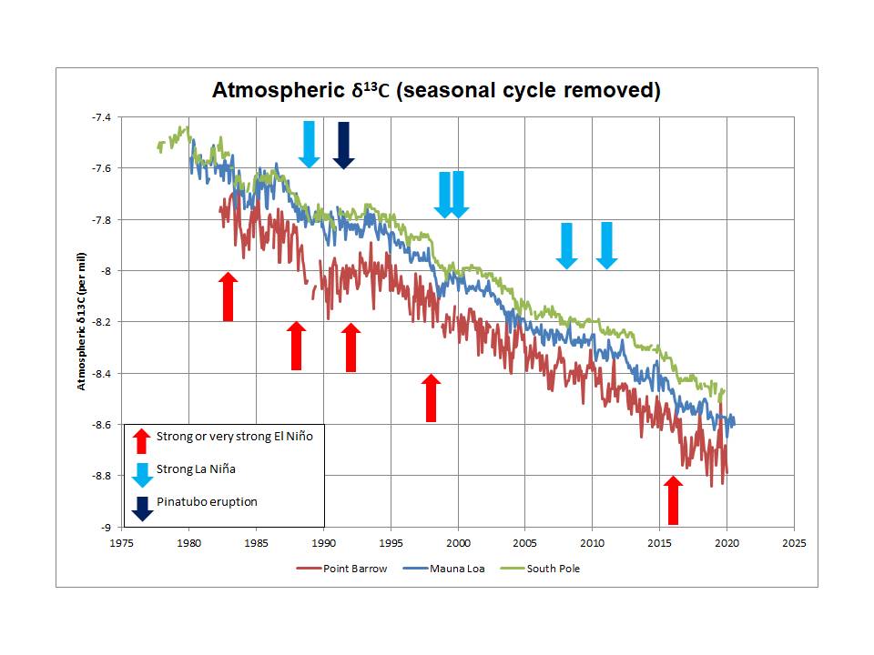 I would argue that the three sets of data track each other, in terms of gradient changes, very well. (The monthly values are from the Scripps Institute where the seasonal cycle has been removed – by Scripps – and hence highlight longer term changes.) There are suggestions of possible time delays of a few months in some places, perhaps even a year, but nothing to support an 8-year lag. The largest short-term drop of 0.2 per mil in the late 80s is not seen anywhere later. Further, the next significant rapid drop occurs in 1998 (at least 10 years later) and actually correlates very well with El Niño. The low point in 1983 (which also corresponds to a strong El Niño) character matches at all three locations very well and the minimum value at Point Barrow is not seen at the South Pole until 1996 at the earliest.
First, I have to clarify that my poorly-worded reference to “rubbish” was with respect to the above charts trying to argue that there is a two year delay in atmospheric CO2 growth between poles and an eight year lag in the 13C/12C ratio (δ13C) of the atmospheric CO2. I was not referring to your original post!
There are several possible reasons for the small latitudinal differences in measured values. In theory, one could be calibration errors between observatories, but that can be ruled out for the Scripps Institute data since they take flask samples at all locations (as well as in situ measurements at some) which are all analyzed at a single laboratory (see https://scrippsco2.ucsd.edu/). The two primary reasons are (i) possible delays in movement of CO2, as speculated in the above charts, and (ii) latitudinal offsets in atmospheric values.
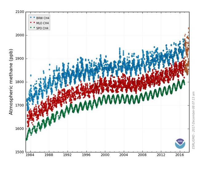
Although the following graph is for atmospheric methane, it provides an excellent example of latitudinal offsets that are not related to timing differences (delays); the observed changes in growth rate occur simultaneously at different latitudes as reflected in the parallel nature of the trends:
Moving on to atmospheric CO2, the 18O/16O ratio (δ18O) also shows latitudinal offsets (parallel trends) which cannot be due to timing differences over the time period covered. See: https://scrippsco2.ucsd.edu/graphics_gallery/isotopic_data/global_stations_isotopic_o18_trends.html
Finally, if we look more closely at δ13C of atmospheric CO2:
Jim, you call your response above a “proof”?
BTW, correlation does not necessarily equal causation. Yeah, that too.
Jim Ross,
It’s now what was tomorrow yesterday.
I’m eagerly awaiting your scientific “proof” that Renee Hannon’s above article merits, in any way, the term “complete rubbish” that you claim.
If you make an absurd—let alone offensive—comment, be prepared to be called out for it.
Waiting for what you are happy to provide . . .
Renee
“Another interesting observation on the mixing between poles. There is a 2-year pole equilibration between CO2 and 6 years for d13CO2 isotopes”. Thanks for the charts.
This is an interesting one.
The first chart I attached identified population and therefore CO2 emission location. The NH is about 90% of global emissions.
Reaching equilibrium, and reaching the same value are two completely separate things.
Atmospheric transport between the hemispheres happens quickly. The rise and fall on both of your charts identifies a close near real time similarity.
What your charts identify is the dilution of the NH volume of CO2 as it travels south and mixes with a greater air mass that has lower emissions. That portion of the atmosphere that makes contact with ocean and biosphere will both loose and gain some CO2 along the way. Not all of the atmosphere makes contact.
So the atmospheric distribution occurs quickly, but dilution drops the mixed values. During that transport atmospheric temperature changes the most important value which no-one talks about – saturation. That is, how close together are the molecules. In a cold atmosphere, the ppm value stays constant but the molecules move closer together. It is the “blanket effect” of increased CO2 that is the key to the IPCC warming claim.
Therefore the density of CO2 is higher at the poles compared to the equator.
Most importantly, the density of CO2 is highest when the atmosphere cools while entering a glacial phase, and the density lowest during the entry into an inter-glacial. This is the complete opposite to what the IPCC states is happening. I had an article on this subject published in E&E in 2010. We manufacture systems that alter equilibrium’s, and that stimulated my interest in atmospheric science.
Kind regards
IMHO, the term “well mixed” is consistent, in the limit, with the second of these, but not the first.
Given that atmospheric CO2 concentration in ppm is on gradually increasing slope over time (ref: Mauna Loa observatory “Keeling curve”), “equilibrium” in the exact definition in this case is impossible.
“equilibrium” in the exact definition in this case is impossible.
Agreed. The total system is so large and dynamic with various and changing thermal zones and seasonal changes, coupled to an active transport system. Its never going to happen.
Regards
Supporting such a claim depends on an agreement on the definition of “well mixed.”
If Antarctica melts, we could house another few billion.
The peak and decline in seasonal CO2 invariably is in May in the NH.
https://wattsupwiththat.com/2021/06/11/contribution-of-anthropogenic-co2-emissions-to-changes-in-atmospheric-concentrations/
Hi Clyde
Mauna Loa is not the entirety of the NH, it is a little island in the middle of an ocean that measures the mixed atmosphere during transport.
See attached chart = mid to late April. This records the changing of circulation patterns etc.
Regards
Chart attached
Renee
Thank you for an outstanding report.
Regards
This (10Be, GCR proxy) may be relevant for the same period.
Why so many words, so may fiddly little graphs? What is it all about?
All anyone needs is even just a rudimentary understanding of Soil Organic Material (SOM) where it comes, where it goes..
Start by winding the clock back to the previous interglacial when sweetness, light, loveliness and plants prevailed. Not dissimilar to The Holocene in fact or prior to when the Sahara was created.
Large areas of Earth land surface would have been green and growing and, contrary to popular opinion but it bu88ers me why, the plants would have been actually laying and accumulating organic material in the soil they were growing in.
They would have creating what is nowadays called “A Horizon” = organic rich dark/black coloured soil.
At a rate of between 1 inch per century (ideal conditions) down to 1 inch per millennium
A combination of sunlight strength, soil trace-element availability (fertility) and CO2 levels would have maintained an even keel.
(The plants, via the SOM look after their own water – and water controls the climate)
Over time, soil fertility (the ultimate limiter) declines and so do the plants and where there are no plants, ice gradually encroaches from the poles.
The ice would cover the SOM and because all microbial life effectively stops below 5°C, the ice-covered SOM remains in limbo. (Permafrost)
Previously bacterial decomposition would have released CO2 from that SOM – thus you see a lovely little (negative) feedback loop control plant growth and CO2 levels.
Thing to note is that decomposition is a slower process than accumulation.
It HAS to be lest there’d never be any fertile soil anywhere on the planet any where ever.
The ice will grow as close to the Equator as El Sol allows it but around that band are few plants to continue the growth, accumulation and slow decomposition of the SOM there.
What plants are there will continue absorbing but mostly CO2 levels will be pulled down by simple rainfall (Carbonic Acid) – being frozen into the ice or falling into what ocean was left exposed
THEN, for whatever reason, the ice melted and all that buried and frozen SOM kicked back into life – hoisting the CO2 level back to where they were and what is recorded in the ice – at that nice level that keeps the plants alive
And there you have a (as brief as I could make it) description for the shape of the graph we see in the Figs 1, 2 and 3 above
Anything more is just the counting of Dancing Angels and can only lead to squabbles and fights.
Especially amongst folks who don’t know, or don’t want to know, about SOM and plants and how via the control those 2 things exert on water, how plants effectively control the climate.
All that’s really left to suss is what ‘broke the ice’
was it volcanoes (possibly and explains some of the CO2 rise?
or
gradual accumulation of dust lifted from the unfrozen regions lowering the Albedo of the ice and that’s what melted it?
Pieter Tans of NOAA claims that the soil organic matter (SOM) participating in the large fluctuations in net CO2 emission into the atmosphere, the slope of the Keeling curve of atmospheric CO2, is limited to the shallow soils of the tropical rain forests, holding only a small amount of carbon compared to the atmosphere and hence not participating in multi-decadal fluctuations.
It appears he claims this in order to dismiss any claims such as yours that there is a biological regulator system of the atmospheric CO2 level. Does he know what he is talking about?
Why have the ice sheets only accumulated during several (5) eposides that account for less than 75% of duration while plants kept growing for much longer intervals over that 75+% of all time?
<i>Over time, soil fertility (the ultimate limiter) declines and so do the plants and where there are no plants, ice gradually encroaches from the poles.</i>
We’re at the tail end of our own interglacial and soil fertility seems to be doing just fine.
“Antarctic CO2 data does not even recognize the 8.2 kyr event”
The Vostok temperature proxy series shows a huge warm spike at 8.2kyr BP.
The Vostok spike at the 8.2 kyr event is an outlier. Vostok is also one of the lowest resolution ice core datasets in the Antarctic due to low snow accumulation rates as well as the poor sampling rate.
Renee
Thanks for the great article!
Do current leaf stomatal densities lie correctly on the calibration curve of stomatal density with CO2 concentration, now of a little over 400 ppm?
Hatter,
There are studies that have exposed plants to current and elevated CO2 concentrations. One interesting study used 350, 420, 490 and 560 ppm CO2; representing the years 1987, 2025, 2051, and 2070, respectively (RCP4.5 scenario). This study did demonstrate that a species responded non-linearly to increases in CO2 concentration when exposed to decadal changes in CO2.
https://link.springer.com/article/10.1007/s00425-020-03343-z
Different species can have different calibrations and some species are limited for palaeoatmospheric pCO2 at levels much higher than 400 ppm. Again, the response may not be linear, but using “datasets tuned with additional data points from superambient experiments, extrapolation beyond the historical herbarium datasets will allow estimation of palaeoat- mospheric pCO2 levels much higher than 400 ppm.”
https://link.springer.com/article/10.1007/s00425-020-03343-z
Renee,
Interesting post, thank you for compiling….minor edit, you write:
“Wagner, 2004, demonstrated CO2 from stomata obtained from different continents and plant species show highly comparable fluctuations during the Younger Dryas, the 8.2 kyr cooling event and the LIA. He states that the agreement of the stomatal frequency records is Northern Hemispheric in nature and not a local continental signature.”
Wagner (Friederike) is a woman.
nvw,
Thanks for pointing out!
This is a very good article (and good comments on it too).
However, I’m just a bit despondent that it feels like we’ve pretty much lost the debate on “climate change”.
There *are* lakes drying up all over the world that the warmists can point to and say “see? Told you so.”
I just think that if we consider man-made climate change as “the Big Lie”, wasn’t it Goebbels who said that “a big lie told often enough becomes the truth”? I think that’s what we are seeing now – the *relentless* hammering of man-made climate change by the MSM, and Joe Average just doesn’t have the brainpower or energy to see otherwise.
Long story short – **we can’t get “cut-through”** to get our message across.
Ok, the “silver lining” is that now very few people believe all that the MSM tell them.
However – I think that the world swallowed the “climate change” Kool-Aid *before* they became skeptical of the MSM. If they had woken up to the MSM *first* then our job would be a *lot* easier. Just my 2c worth…….
Does anyone have any evidence to suggest that our side is winning?
If so, I’d love to see it.
– j.g.