Guest essay by Kip Hansen
 What we call a graph is more properly referred to as “a graphical representation of data.” One very common form of graphical representation is “a diagram showing the relation between variable quantities, typically of two variables, each measured along one of a pair of axes at right angles.”
Here at WUWT we see a lot of graphs — all sorts of graphs of a lot of different data sets. Here is a commonly shown graph offered by NOAA taken from a piece at Climate.gov called “Did global warming stop in 1998?” by Rebecca Lindsey published on September 4, 2018.

I am not interested in the details of this graphic representation — the whole thing qualifies as “silliness”. The vertical scale is in degrees Fahrenheit and the entire range change over 140 years shown is on the scale 2.5 °F or about a degree and a half C. The interesting thing about the graph is the effort of drawing of “trend lines” on top of the data to convey to the reader something about the data that the author of the graphic representation wants to communicate. This “something” is an opinion — it is always an opinion — it is not part of the data.
The data is the data. Turning the data into a graphical representation (all right, I’ll just use “graph” from here on….), making the data into a graph has already injected opinion and personal judgement into the data through choice of start and end dates, vertical and horizontal scales and, in this case, the shading of a 15-year period at one end. Sometimes the decisions as to vertical and horizontal scale are made by software — not rational humans — causing even further confusion and sometimes gross misrepresentation.
Anyone who cannot see the data clearly in the top graph without the aid of the red trend line should find another field of study (or see their optometrist). The bottom graph has been turned into a propaganda statement by the addition of five opinions in the form of mini-trend lines.
Trend lines do not change the data — they can only change the perception of the data. Trends can be useful at times [ add a big maybe here, please ] but they do nothing for the graphs above from NOAA other than attempt to denigrate the IPCC-sanctioned idea of “The Pause”, reinforcing the desired opinion of the author and her editors at Climate.gov (who, you will notice from the date of publication, are still hard at it hammer-and-tongs, promoting climate alarm). To give Rebecca Lindsey a tiniest bit of credit, she does write “How much slower [ the rise was ] depends on the fine print: which global temperature dataset you look at”…. She certainly has that right. Here is Spencer’s UAH global average lower tropospheric temperature:

One doesn’t need any trend lines to be able to see The Pause that runs from the aftermath of the 1998 Super El Niño to the advent of the 2015-2016 El Niño. This illustrates two issues: Drawing trend lines on graphs is adding information that is not part of the data set and it really is important to know that for any scientific concept, there is more than one set of data — more than one measurement — and it is critically important to know “What Are they Really Counting?”, the central point of which is:
So, for all measurements offered to us as information especially if accompanied by a claimed significance – when we are told that this measurement/number means this-or-that — we have the same essential question: What exactly are they really counting?
Naturally, there is a corollary question: Is the thing they counted really a measure of the thing being reported?
I recently came across an example in another field of just how intellectually dangerous the cognitive dependence (almost an addiction) on trend lines can be for scientific research. Remember, trend lines on modern graphs are often being calculated and drawn by statistical software packages and the output of those packages are far too often taken to be some sort of revealed truth.
I have no desire to get into any controversy about the actual subject matter of the paper that produced the following graphs. I have abbreviated the diagnosed condition on the graphs to gently disguise it. Try to stay with me and focus not on the medical issue but on the way in which trend lines have affected the conclusions of the researchers.
Here’s the big data graph set from the supplemental information for the paper:
Note that these are graphs of Incidence Rates which can be considered “how many cases of this disease are reported per 100,000 population?”, here grouped by 10-year Age Groups. They have added colored trend lines where they think (opinion) significant changes have occurred in incident rates.

[ Some important details, discussed further on, can be seen on the FULL-SIZED image, which opens in a new tab or window. ]
IMPORTANT NOTE: The condition being studied in this paper is not something that is seasonal or annual, like flu epidemics. It is a condition that develops, in most cases, for years before being discovered and reported, sometimes only being discovered when it becomes debilitating. It can also be discovered and reported through regular medical screening which normally is done only in older people. So “annual incidence” may not a proper description of what has been measured — it is actually a measure of “annual cases discovered and reported’ — not actually incidence which is quite a different thing.
The published paper uses a condensed version the graphs:

The older men and women are shown in the top panels, thankfully with incidence rates declining from the 1980s to the present. However, as considerately reinforced by the addition of colored trend lines, the incident rates in men and women younger than 50 years are rising rather steeply. Based on this (and a lot of other considerations), the researchers draw this conclusion:

Again, I have no particular opinion on the medical issues involved…they may be right for reasons not apparent. But here’s the point I hope to communicate:

I annotate the two panels concerning incidence rates in Men older than 50 and Men younger than 50. Over the 45 years of data, the rate in men older than 50 runs in a range of 170 to 220 cases reported per year, varying over a 50 cases/year band. For Men < 50, incidence rates have been very steady from 8.5 to 11 cases per year per 100,000 population for 40 years, and only recently, the last four data points, risen to 12 and 13 cases per 100,000 per year — an increase of one or two cases [per 100,000 population per year. It may be the trend line alone that creates a sense of significance. For Men > 50, between 1970 and the early 1980s, there was an increase of 60 cases per 100,000 population. Yet, for Men < 50, the increased discovery and reporting of an additional one or two cases per 100,000 is concluded to be a matter of “highest priority” — however, in reality, it may or may not actually be significant in a public health sense — and it may well be within the normal variance in discovery and reporting of this type of disease.
The range of incidence among Men < 50 remained the same from the late 1970s to the early 2010s — that’s pretty stable. Then there are four slightly higher outliers in a row — with increases 1 or 2 cases per 100,000. That’s the data.
If it were my data — and my topic — say number of Monarch butterflies visiting my garden annually by month or something, I would notice from the panel of seven graphs further above, that the trend lines confuse the issues. Here it is again:
[ full-sized image in new tab/window]
If we try to ignore the trend lines, we can see in the first panel 20-29y incidence rates are the same in the current decade as they were in the 1970s — there is no change. The range represented in this panel, from lowest to highest data point, is less than 1.5 cases/year.
Skipping one panel, looking at 40-49y, we see the range has maybe dropped a bit but the entire magnitude range is less than 5 cases/100,000/year. In this age-group, there is a trend line drawn which shows an increase over the last 12-13 years, but the range is currently lower than in the 1970s.
In the remaining four panels, we see “hump shaped” data, which over the 50 years, remains in the same range within each age-group.
It is important to remember that this is not an illness or disease for which a cause is known or for which there is a method of prevention, although there is a treatment if the condition is discovered early enough. It is a class of cancers and incidence is not controlled by public health actions to prevent the disease. Public health actions are not causing the change in incidence. It is known to be age-related and occurs increasingly often in men and women as they age.
It is the one panel, 30-39y , that shows an increase in incidence of just over 2 Cases/100,000/year that is the controlling factor that pushes the Men < 50 graph to show this increase. (It may be the 40-49y panel having the same effect.) (again, repeating the image to save readers scrolling up the page):
Recall that the Conclusion and Relevance section of the paper called this “This increase in incidence among a low-risk population calls for additional research on possible risk factors that may be affecting these younger cohorts. It appears that primary prevention should be the highest priority to reduce the number of younger adults developing CRC in the future.”
This essay is not about the incidence of this class of cancer among various age groups — it is about how having statistical software packages draw trend lines on top of your data can lead to confusion and possibly misunderstandings of the data itself. I will admit that it is also possible to draw trend lines on top of one’s data for rhetorical reasons [ “expressed in terms intended to persuade or impress” ], as in our Climate.gov example (and millions of other examples in all fields of science).
In this medical case, there are additional findings and reasoning behind the researchers conclusions — none of which change the basic point of this essay about statistical packages discovering and drawing trend lines over the top of data on graphs.
Bottom Lines:
- Trend lines are NOT part of the data. The data is the data.
- Trend lines are always opinions and interpretations added to the data and depend on the definition (model, statistical formula, software package, whatever) one is using for “trend”. These opinions and interpretations can be valid, invalid, or nonsensical (and everything in between)
- Trend lines are NOT evidence — the data can be evidence, but not necessarily evidence of what it is claimed to be evidence for.
- Trends are not causes, they are effects. Past trends did not cause the present data. Present data trends will not cause future data.
- If your data needs to be run through a statistical software package to determine a “trend” — then I would suggest that you need to do more or different research on your topic or that your data is so noisy or random that trend maybe irrelevant.
- Assigning “significance” to calculated trends based on P-value is statistically invalid.
- Don’t draw trend lines on graphs of your data. If your data is valid, to the best of your knowledge, it does not need trend lines to “explain” it to others.
# # # # #
Author’s Comment Policy:
Always enjoy your comments and am happy to reply, answer questions or offer further explanations. Begin your comment with “Kip…” so I know you are speaking to me.
As a usage note, it is always better to indicate who you are speaking to as comment threads can get complicated and comments do not always appear in the order one thinks they will. So, if you are replying to Joe, start your comment with “Joe”. Some online periodicals and blogs (such as the NY Times) are now using an automaticity to pre-add “@Joe” to the comment field if your hit the reply button below a comment from Joe.
Apologies in advance to the [unfortunately] statistically over-educated who may have entirely different definitions of common English words used in this essay and thus arrive at contrary conclusions.
Trends and trend lines are a topic not always agreed upon — some people think trends have special meaning, are significant, or can even be causes. Let’s hear from you.
# # # # #
Discover more from Watts Up With That?
Subscribe to get the latest posts sent to your email.
Trend lines work for dependent variables only. X makes Y. Then you get a trend which is y = mx + b. Since time does not make climate, time series trend have no meaning.
Time is often a dependent variable… like exponential decline curves.
Signal processing engineers don’t ‘draw’ trend lines, we ‘draw’ sine waves. (we probably haven’t drawn them since Fourier’s time, we calculate them).
A trend line as drawn in the above diagrams is simply a sine wave whose period is far far longer than the data window we are looking at.
IOW, a trend line is guessing about data we don’t have, both in the future and in the past.
Formally, we know nothing about any sine wave whose period is more than 1/2 that of the length of the data we are looking at.
Trend lines are very bad signal processing technique, and belong in the same category as Mann’s attempt at signal processing resulting in bogus hockey sticks.
+!
Trying to explain the pause, I used this to explain why the was pause was real and important.
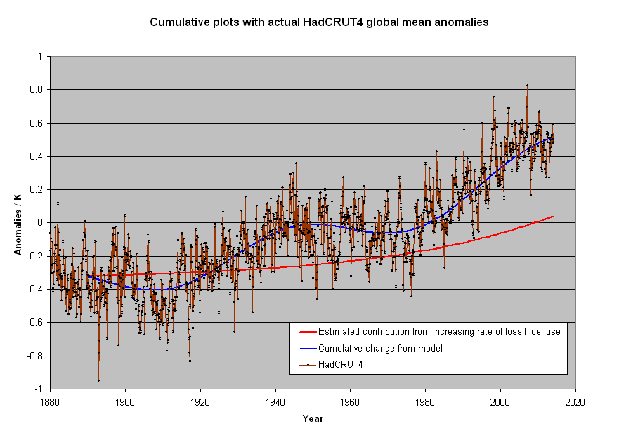
Where one third of human emissions occurred in even this simple model of a constant warming rate plus a sinusoidal with 60 year period and 1/3 C of a degree warming due to acceleration since 1950, is where the fit is the poorest. It makes it less reasonable to claim both human CI2 and temperature are going up with time so it must be human emissions.
PS Similar issue with the term modelling. Its a quantitative argument, not divining.
Kip, I’m sorry, I didn’t read all the comments, so maybe someone else said this.
Regarding the cancer incidence graphs, did you read the methods? The authors used a statistical program, Joinpoint Regression, which is specifically designed to test for changes in trends. Unless you want to tell us how this tool is being wrongly used, or that it’s inadequate for the purpose, I’m not sure what your point is.
There’s nothing wrong with trend lines per se, as long as they are used carefully with the correct statistic (regression vs. correlation, for example), and the assumptions of that statistic are met. Interpreting the line is the next step. Of course, if the wrong beginning and endpoints are used, or not enough points, or if the data need to be transformed, or whatever, it can weaken the statistic or the argument. But unless one simply draws a line where one feels it’s appropriate, it’s not an “opinion,” it represents a statistical relationship among the points, and additional numeric information about the quality (slope and its direction) and strength of the relationship between variables.
You are attacking something that has commonly been used for at least 150 years to aid in the visual communication of a statistic. Why?
Kristi ==> If you don’t understand why I have objections to the practice, I must assume I failed to communicate it properly.
The problem is that trend lines are being drawn where “oine feels appropriate”.
Having statistical packages draw ones lines is worse, not better.
The better question is “Are the trends found by the stats software Minimally Clinically (in this case, public health-wise) Important?”
I stated several times, I am not involved in the medical issue — only the trend lines — drawing of anfd use of — issue.
Goods to see comments from you here again.
Kip,
You stated that trend lines were a matter of opinion. When you use statistics properly, it removes the “opinion” part. The statistics to use are often decided before the data are even collected, so where does the “opinion” come in? Opinion may influence the best statistical test or program to use, but that is not the same as deciding where the trend lines fall. “Joinpoint fits the selected trend data (e.g., cancer rates) into the simplest joinpoint model that the data allow. The resulting graph is like the figure below, where several different lines are connected together at the “joinpoints.” The figure is here: https://surveillance.cancer.gov/joinpoint/Joinpoint_Help_4.5.0.1.pdf, which also explains the options one can select in the program, its mathematical basis, etc. The program selects where to draw the lines.
Whether the trends are “minimally clinically important” is about the interpretation of the trends, not about drawing the lines themselves.
In your climate example, presumably the trend lines for the upper graph were selected based on the dataset used and the years of the so-called “pause,” for comparison. The lower graph then uses the same length of the pause trend line to look at previous blocks of the same length as the “pause.” One could argue that this is not the right length of time, or doesn’t cover the right start and stop point of the “pause,” or whatever, but the point is that the sequential trend lines are not of arbitrary length, and not merely opinion.
“The interesting thing about the graph is the effort of drawing of “trend lines” on top of the data to convey to the reader something about the data that the author of the graphic representation wants to communicate. This “something” is an opinion — it is always an opinion — it is not part of the data.”
The trend line is not part of the data, no, but there would be no trend line without the data. The line is meaningful, a visual and mathematical representation of the data, so how is that “opinion”? An opinion would be, “The trend is very steep.” Where is the opinion in, “Based on this data, between 1880 and 2017 the global surface temperature has risen an average of 0.13 F per decade”? Are all statistics simply opinions?
“If your data needs to be run through a statistical software package to determine a “trend” — then I would suggest that you need to do more or different research on your topic or that your data is so noisy or random that trend maybe irrelevant.”
What would you suggest as a replacement? Eye-balling it, and saying, “Well, it seems to go up”?
While there are plenty of examples of abuse of trend lines, it’s true that I honestly don’t see your underlying motive for attacking their use in general. Just like a histogram or a pie chart, trend lines are a useful way of visually communicating mathematical relationships. You are right, you haven’t (to my mind) adequately explained why you think trend lines are “opinions.”
I stopped commenting (and come here seldom in general) because I got so tired of seeing the same old deprecation of large groups of people, the same disparagement of most of the scientific community, the same old specious arguments… it got frustrating and boring when there are so few interesting discussions. And one gets tired of being personally attacked for one’s views. WUWT is a waste of my time.
But you’ve usually been civil to me, and I’ve appreciated that. Take care, Kip!
Kristi ==> Always glad to see you here — I was quite serious that I was not taking up the medical issues of the CRC paper, only their dependence on (or insistence on) trends produced by a stats package.
Not intended to critic their paper in general — just that one point. Yes, they started off looking for “trends”and my opinion is that it led them astray be cause their trends were ‘significant”…etc etc.
There is a lot of trend nonsense in many fields, CliSci is trend crazy.
You need to read my whole linked series on the Button Collector and the piece I did on Andy Revkins NY Times blog to see the big picture.
Trend lines are opinions because they depend so much on the start and end points (chosen to match the opinion of the line drawer) and on the type of trend calculated.
If you missed it, see https://www.xkcd.com/2048/
Kip,
As I said, trends can be abused. All statistics can be improperly applied and interpreted. That’s why there are rules in science about the way statistics are used. I’ve seen on WUWT trend lines applied to data that look to me as if the assumptions weren’t met (e.g. normal distribution, homoscedascity, etc.), but that doesn’t mean everyone does it. Sometimes it’s not even clear that people know the difference between a correlation and a regression or what inferences can be drawn from each. That’s the problem when anyone can stick some data into Excel and run a test on it without knowing anything about statistics. But it’s not safe to assume that’s the case across the board, for all scientists who use trend lines. Do you know, for example, that the author of the climate paper chose the data to use after she saw the trends different starting/ending dates would produce? After all, she could have chosen to start the main trend at 1910 or extended the “pause” to 2016 and would have gotten more of a slope.
Krisii: “Where is the opinion in, “Based on this data, between 1880 and 2017 the global surface temperature has risen an average of 0.13 F per decade”? Are all statistics simply opinions?”
The trend line does *not* show that the global surface temperature has risen since it is based on an average value which loses the data needed to understand if the global surface temperature has risen at all. The average hides whether Tmax is going up, whether Tmin is going up, or if a combination of the two is happening. Tmax going up might be bad and Tmin going up might be good. The trend line of the average can’t tell you either.
That’s one of the pitfalls of trend lines. If you don’t understand the data then the trend line can “fool” you into an interpretation that is totally at odds with the data.
Tim,
It depends on what one wants to assess. If one is trying to find out if the globe is warming as a whole over time, one would use averages and anomalies. Tmax and Tmin don’t matter to the whole except through their impact on the average at each weather station. If Tmax is rising on average as the same rate Tmin is falling, the average will stay the same. This, too, may be meaningful, but looking at one or the other will not tell you whether the globe as a whole is getting warmer through the decades. If, on the other hand, one is trying to find out if the minimum temperature for February at Casper, WY is going up or down over the years, one could use the absolute minimum temp in Feb. for each year, or the average of the Feb. daily minimums for each year.
Tmax going down and Tmin going up might be bad, too, in some areas, depending on what effect one is interested in. For example, minimum winter temperatures control how far north some destructive insects are able to survive. In some/most cities, extreme heat kills more people per degree rise than extreme cold kills per degree fall (because it is cold in general that tends to kill through effects on disease, while extreme heat more often causes acute bodily harm), in others the opposite is true. It is up to the researcher to choose what is most meaningful for the study.
A trend in average temperature change over 150 years suggests the globe’s heat budget is changing even if the trend is down in some periods as long as the changes from year to year are not so great that the signal is lost in the noise. A trend line alone is not enough to assess this, and sometimes adding a trend line can be improper, which is why there are rules for using and reporting trend lines (which are simply graphical representations of statistics). I don’t know if the author of the climate research above followed the rules, and I’m not going to simply assume she did or didn’t (unless it was peer-reviewed and published in a reputable journal, and even then I might try to confirm it myself). Assuming she did something wrong is a mistake, too. There are far too many incidents of assuming researchers did poor work just because it didn’t support readers’ biases, or good work because it did.
It’s not just understanding the data that’s important, it’s also understanding the proper use of statistics. Often readers have to trust that scientists know what they are doing. Unless there is documented evidence for widespread scientific misconduct or laxity within a field (which has not been demonstrated in climate science), I see little reason to mistrust most researchers – though even the best may make errors or get erroneous results by chance, which is why assessing a body of research is better than relying on any one paper. On the other hand, there is reason to be skeptical of how science is reported by the media and those without expertise in the field.
Kristi: “If one is trying to find out if the globe is warming as a whole over time, one would use averages and anomalies. Tmax and Tmin don’t matter to the whole except through their impact on the average at each weather station.”
If the increase in Tmin keeps below the point where it causes ice and snow to melt over wide ranges of the globe then Tmin certainly matters. If Tmax is actually going down then this negates all the claims of the AGW alarmists that we are going to see a decrease in food production, especially in grains which is a large part of the global food supply. Grains are negatively impacted by Tmax going above 90degF to 95degF. If Tmax is going down or even staying stable it is a *big* deal.
“Tmax going down and Tmin going up might be bad, too, in some areas, depending on what effect one is interested in. For example, minimum winter temperatures control how far north some destructive insects are able to survive.”
Can you point to someplace on the globe where destructive insects have made the place inhabitable? With today’s ag capability the ability to control destructive insects is far greater than our ability to control CO2 production.
“A trend in average temperature change over 150 years suggests the globe’s heat budget is changing even if the trend is down in some periods as long as the changes from year to year are not so great that the signal is lost in the noise.”
If some regions are seeing cooling and some are seeing warming then is the *globe’s” heat budget changing? Or just some regions? How do you tell from a “global” average?
“It’s not just understanding the data that’s important, it’s also understanding the proper use of statistics.”
Applying statistics to an “average” is, in almost every situation, an improper use of statistics. Once you take the average then you have absolutely no idea of what is actually happening in reality. You can calculate all the statistics from the average that you want, the statistics only tell you what is happening to the average.
It’s like taking 10 groups of 1000 steel girders and calculating an average length for each group. Plotting that average and developing a trend line from a regression analysis will tell you what? You will still have no idea what the longest and shortest lengths are so you can’t design a fish plate to connect them that will work in all situations. It’s the same with using an “average” temperature for the globe. You can plot and calculate all you want with that “average” global temperature, you still won’t know what is going on around the globe.
Tim,
“If the increase in Tmin keeps below the point where it causes ice and snow to melt over wide ranges of the globe then Tmin certainly matters. ”
“Budget” was the wrong word. How about “index”?
When you are trying to find out if the global temperature is increasing over time, as in the first graph, the processes don’t matter. What you do is look at anomalies for every station, and average them over the course of a year, then average all those to find a global average (that’s oversimplifying, obviously, but I’m not going to get into a long explanation here). Plot the yearly global averages, run a regression, and you have a trend.
“If Tmax is actually going down then this negates all the claims of the AGW alarmists that we are going to see a decrease in food production, especially in grains which is a large part of the global food supply. ”
It’s far more complicated than that. For example, If Tmax goes down, you may have a shorter growing season in some areas if the ground takes longer to thaw and freezes early. You could also see a change in precipitation patterns if the air holds less water. The systems are variable and complex.
“Can you point to someplace on the globe where destructive insects have made the place inhabitable? With today’s ag capability the ability to control destructive insects is far greater than our ability to control CO2 production.”
I assume you mean uninhabitable, but that’s not the point. My point was that there’s potentially a very high economic cost when destructive insect expand their range and/or become more prolific. The bark boring beetles that killed thousands of acres of forest in the Rockies are a good example. Emerald ash borer populations are limited by cold in the north. These insects cause billions of dollars worth of damage every year. I’m not as familiar with food crop pests, but I imagine there exist similar environmental limits. Yes, to some extent it’s possible to control many pests, but control, too, comes at a cost, and for some, particularly subsistence or small-scale farmers in the developing world, these costs are simply too high. Again, it’s a complex subject.
An extremely wide array of plants and animals are changing their ranges and behavior in response to climate change. That is well-established.
“If some regions are seeing cooling and some are seeing warming then is the *globe’s” heat budget changing? Or just some regions? How do you tell from a “global” average?”
The global average is important because that’s what we look at to see if the planet is warming. As more heat is trapped, the planet warms. (Of course, much of the extra heat is absorbed by the oceans, and we don’t have a very good understanding of where it goes – but we do know that they are generally warming.)
“Applying statistics to an “average” is, in almost every situation, an improper use of statistics.”
I disagree. An average is simply a number. Looking at a trend in a time series of averages is perfectly legitimate. Here, in Figure 2, is an example for an introductory course on statistics, published in Journal of Statistics Education http://jse.amstat.org/v21n1/witt.pdf. (A good example for Kip, too!) Note Table 1. It turns out that a quadratic equation for the regression is better than linear, as the rate of decline in Sept. Arctic sea ice extent is increasing.
“You can plot and calculate all you want with that “average” global temperature, you still won’t know what is going on around the globe.”
If you mean the regional variation, that’s perfectly true. That’s a whole nuther ball game!
Kristi:
“The global average is important because that’s what we look at to see if the planet is warming.”
But it does *not* tell you if the globe is warming. If only one region is warming, say central Africa, and the rest are static you it will see an increase in the global average. So exactly what does the global average actually tell you? Again, taking an average *loses* valuable data. It would be far better to come with solutions for the areas that are warming than trying to shoehorn everyplace into a one-size-fits-all solution.
” Looking at a trend in a time series of averages is perfectly legitimate. ”
Taking an average of MINIMUM sea ice extent in Sept and doing a regression of a time series only tells you something about the minimum extent in Sept. What does it tell you about the *maximum* extent? Nothing.
“If you mean the regional variation, that’s perfectly true. That’s a whole nuther ball game!”
The globe is made up of regions. If you don’t know what is going on in the various regions then you really don’t know what is going on with the globe.
Tim,
No one proposes that the whole planet is warming uniformly. Some regions may not be warming at all, and some may even be cooling due to changed weather patterns (due, for example, to increased Arctic ice melt and its effects on ocean currents – mind you, I don’t know if there is regional cooling happening). It IS the average that one has to look at to see if there is an effect of increased atmospheric CO2 on the TOTAL global energy exchange with outer space. I don’t know how that can be made clearer.
Kristi: ” It IS the average that one has to look at to see if there is an effect of increased atmospheric CO2 on the TOTAL global energy exchange with outer space. I don’t know how that can be made clearer.”
If there is regional cooling and warming then the *average* global energy exchange with space is meaningless. And if it is weather that is causing the cooling trends in some places then why isn’t it weather that is causing heating in other places?
If you don’t believe regional cooling is happening then google the term “global warming hole”.
As far as the energy budget, as the Earth warms it radiates *more* IR (see the S-B equation). Yet we are being asked to believe that doesn’t happen with the Earth. We are to believe that as the Earth warms it radiates at a fixed rate that doesn’t change so that the Earth’s temperature can continually go up. There is something wrong with that belief.
Tim,
When I say “the planet,” I include the atmosphere. Without it, you are right: the Earth would simply radiate heat back into space. Fortunately, we have an atmosphere, making the planet habitable. But adding CO2 changes the atmosphere, making it retain more heat. That’s the whole point. I thought you’d heard.
I’m not going to argue about this any more. It’s going nowhere. The physics is sound, the observational evidence is there…the planet is warming.
Kristi:
“But adding CO2 changes the atmosphere, making it retain more heat”
How does an atmosphere retain heat? If a molecule in the atmosphere gains energy, i.e. heat, then it will radiate that extra energy, it will lose the heat in a collision with another molecule, or it will change position (usually rising – e.g. hot air). All of these will contribute to the heat being lost, e.g. hot air rising to where it is colder.
“I’m not going to argue about this any more. It’s going nowhere. The physics is sound, the observational evidence is there…the planet is warming.”
In other words, don’t question the religious dogma. The physics simply do not work. It requires believing that the Earth can warm without losing that extra heat to a colder body (space). Pardon me if I know enough physics to question the religious dogma.
Kip! I agree that trend lines are not the data. But unfortunately the data is not the data either. To illustrate this:
Divide the UAH data point stream into 12 different data point streams, one for each month. If you calculate the standard deviation of each stream you will find that the November stream has much lower standard deviation than the rest and the February stream has the highest std. November points are simply more trustworthy than February points. If you calculate a trendline that treat these two streams as comparable you are making an error. The warming trend in these monthly streams seems to fall in three categories: 0,0147-0,0149 K/a(nnum) for Jan-, Feb-, Sep-, Oct-series; 0,0110-0,0114 K/a for May-, June-, August-series; and 0,0121-0,0131 K/a for Mar-, Apr-, Jul-, Nov-, Dec-series. Adding to this complexity is vulcanos, ENSO and other disturbances But if we are willing to examine the data they seem to be capable of telling us more than if we are not prepared to do so. There is simply no way any single graph can show all details.
Johan ==> The data is not always “the” data — and it does not always represent the thing it is claimed to represent…..you are quite right.
Just a final remark
In climate science you often come across certain known functions,
e.g. I found the speed of warming of Tmax at specific places on earth following a sinusoid, with wavelength 87 years. Similarly, I found rainfall patterns at certain places on earth following the pendulum of clock, from top to bottom 43 years (2 successive Hale cycles) and from bottom to top another 43 years (for the next 2 Hale cycles, making 1 full Gleissberg cycle).
In both the above samples, it follows that you can use a linear trend line for the original to show ‘no trend’ over the relevant wavelength period, i.e. 86.5 years.
I hope this makes sense to some here, like A C Osborn?
Obviously, if you don’t know the cycle time you will get rubbish from a trend line, it might even scare you…
I have been closely examining tide charts for the past several weeks, and applying what Kip is saying in this article to those tide charts, shows clearly the wisdom of what Kip is saying.
Trends are drawn on these charts which completely obscure what is actually shown by the data.
Nicholas ==> For another example of your point, see my essay “Cowtan and Way – The Magician’s ‘Red Scarf Trick’ with Linear Trend Lines” @ur momisugly https://wattsupwiththat.com/2013/11/20/cowtan-and-way-the-magicians-red-scarf-trick-with-linear-trend-lines/
Reminds me of a Pacific island used in alarmist media articles about scary sea level rise. I forgot which one but its record starts just before a large metre dip in tide heights due to the 1998 El Nino. Pretty much a zero trend from 1999 to the present but start from 1997 and you get an alarming trend.
In cartography and geography there is a practice called “vertical exaggeration,” wherein the vertical scale is exaggerated in relation to the horizontal scale, so that a 10-km cross-section with 100 m of relief doesn’t look like a straight line like it would if the two scales were equal.
Instead, the horizontal scale might be 1 cm =1 km, while the vertical scale might be 1 cm = 10 m. Since the ratio of horizontal to vertical scale is 1km:1cm: 10m:1cm, the vertical exaggeration would be 1000m:10m, or 10 to 1.
Does the graphing of time series have a similar concept? If the appropriate scales are used in these plots of anomalies, they can be made to look like a steep mountain of global warming or a smooth surface of pause.
If there is no such name for the concept, one should be invented.
James ==> There are two problems in this category with CliSci graphs. One is exaggeratedly compressed vertical scale, by that I mean the scale top-to-bottom covers minuscule magnitude to make tiny changes appear to be large changes. This is often done intentionally.
The second problem is a software problem — if you have used any software package (MatLab, etc) or used an online graphing engine — such as plot.ly or VisMe — they often auto-magically set the scale to be some little bit larger than the extent of the data….this is a reasonable decision but can be very distorting of data with small changes over time.
Kip, you may have generalized too much, but as respects “climate” graphs, “trends” are meaningless where:
1. The CAUSE of the “trend” is unknown.
2. There are MULTIPLE “causes” of the trend, which have not been separately identified and quantified.
3. The quality of the DATA is NOT FIT for the purpose of identifying meaningful “trends.”
4. The subject being measured is subject to CYCLIC variations that render the available data too short in terms of time to be meaningful, in terms of identifying “trends.”
ALL of these issues apply to virtually every climate “graph” in existence, yet the so-called “climate scientists” like to pretend their “data” has TENTH of a degree precision, when (a) most of what they call “data” ISN’T EVEN DATA, and the precision is orders of magnitude worse than they represent it to be.
AGW ==> I like to take strong positions and let others work through them … some of my “strong” is rhetorical….
And yet trend lines over very short periods of time are the climate “sceptics” bread and butter.
Very few skeptics will put a trend line to a graph. They mostly see the graph as noise. Take 10 data points representing some Y value for each X value year. Give a value of 1 to each of 5 successive years at the beginning. Then give a value of 10 to each of the last 5 remaining years to the present or far right of the graph. Everyone would say the graph represents a tipping point at the end of the 5th year and thus definitely has a trend upward.
Now consider a completely different data set of reordering of the yearly data so that each every other year the value 10 follows a 1 value like this 1, 10, 1, 10, 1, 10, 1, 10, 1, 10,
Now there is no tipping point but the the standard deviation is the same in both. Skeptics would say the 2nd data set is all noise whereas climate scientists would calculate the trend line by least squares regression. If they had done it for the 1st set of data, they would end up with the same trend line for both. However both trend lines are invalid and both graphs are noise.
I should have said only the last graph is noise, but even that can be argued because of some underlying cause of the 1 to 10 cycle of each paired successive year.
I should have said only the last graph is noise.