Guest essay by Mike Jonas
“And what might they be?” – Dr. Leif Svalgaard
For a long time, I have been bitterly disappointed at the blinkered lopsided attitude of the IPCC and of many climate scientists, by which they readily accepted spurious indirect effects from CO2-driven global warming (the “feedbacks”), yet found a range of excuses for ignoring the possibility that there might be any indirect effects from the sun. For example, in AR4 2.7.1 they say “empirical results since the TAR have strengthened the evidence for solar forcing of climate change” but there is nothing in the models for this, because there is “ongoing debate“, or it “remains ambiguous“, etc, etc.
In this article, I explore the scientific literature on possible solar indirect effects on climate, and suggest a reasonable way of looking at them. This should also answer Leif Svalgaard’s question, though it seems rather unlikely that he would be unaware of any of the material cited here. Certainly just about everything in this article has already appeared on WUWT; the aim here is to present it in a single article (sorry it’s so long). I provide some links to the works of people like Jasper Kirkby, Nir Shaviv and Nigel Calder. For those who have time, those works are worth reading in their entirety.
Table of Contents:
1. Henrik Svensmark
2. Correlation
3. Galactic Cosmic Rays
4. Ultra-Violet
5. The Non-Linear System
6. A Final Quirk
Abbreviations
References
1. Henrik Svensmark
Back in 1997, when Henrik Svensmark and Eigil Friis-Christensen first floated their hypothesis on the effect of Galactic Cosmic Rays (GCRs) on Earth’s climate, it shook the world of climate science. But it was going to take a lot more than a shake to dislodge climate science’s autocrats. Their entrenched position was that climate was primarily driven by greenhouse gases, and that consequently man-made CO2 would be catastrophic (the CAGW hypothesis), and they were going to do whatever it took to protect their turf.
Those CAGW scientists were supported by remarkably little evidence. Laboratory experiments had verified the mechanics of CO2 as a greenhouse gas, but there was no empirical evidence that it was a major driver of climate. There were correlations, but inspection showed that temperature change always preceded CO2 change. The only support for CAGW came from climate models which had the assumed effects of CO2 built in. The models gave imaginary projections of what future climate would be like if CAGW was correct, but they could not reproduce past climate.
In 2003, Henrik Svensmark and Nigel Calder in the book The Chilling Stars [1] described how cloud cover changes caused by variations in cosmic rays are a major contributor to global temperature changes, and stated that human influences had been exaggerated.
Empirical evidence supported their theory, which they called Cosmoclimatology [2][3], and Henrik Svensmark had conducted an experiment to verify its mechanics. So Henrik Svensmark was fully justified in claiming that Cosmoclimatology “is already at least as secure, scientifically speaking, as the prevailing paradigm of forcing by variable greenhouse gases.”.
The next step was to publish in a peer-reviewed journal. Henrik Svensmark and his team at the Danish National Space Center (DNSC, now DTU Space) submitted a straightforward paper describing their experimental results to a peer-reviewed journal. They were stunned when the climate science tsars closed ranks and the paper was rejected. At this point, the clean-shaven Henrik Svensmark, as a kind of protest, decided not to shave until the paper was published. He had a pretty impressive beard by the time Experimental evidence for the role of ions in particle nucleation under atmospheric conditions [4] was eventually published in Proceedings of the Royal Society A. The process had taken 16 months.
Here we are, twenty years after the GCR hypothesis was first floated, and the CAGW paradigm is still in place and virtually unscathed. This is in spite of increasing evidence supporting Cosmoclimatology and in spite of the epic failure of climate models to predict climate. Paradigm protection has been seen many times in science, but I wonder whether it has ever been as corrupt and as extreme as it currently is in climate science.
I should have mentioned that there was strong opposition against experimental testing of Cosmoclimatology. Think about that – scientists trying to prevent a thoery being tested – and I think you will agree that my use of the word “corrupt” in the previous paragraph was justified.
2. Correlation
There is a strong correlation between solar activity and Earth’s climate. Jasper Kirkby wrote a wide-ranging paper, Cosmic Rays and Climate [5] in which he described the background to the planned CLOUD experiment at CERN, which would test the Cosmoclimatology theory.
In the paper, Jasper Kirkby presented a number of graphs which showed correlations between GCRs and climate. Of course, correlation is not causation, but as GCRs are controlled by solar activity the correlations do show a strong relationship between solar activity and Earth’s climate.
From the paper:
Over 500 million years:

Figure 1. Correlation of cosmic rays with temperature over the past 500 million years. [The paper’s Fig.11].
Note: The GCR flux varies as the solar system passes through the spiral arms of the Milky Way.
Over 12,000 years:

Figure 2. Correlation of GCR variability with ice-rafted debris events in the North Atlantic during the Holocene. [The paper’s Fig. 8].
The paper explains how the 14C and 10Be records are independent proxies for GCRs, and how ice-rafted debris relates to climate.
Over 3,000 years:

Figure 3. Correlation of δ18O and Δ14C with rainfall. [The paper’s Fig. 9].
The paper explains how Δ14C is a proxy for GCRs, and δ18O is a proxy for rainfall.
Over 2,000 years:

Figure 4. Correlation of GCRs with Central Alps temperature over the last two millenia. [The paper’s Fig. 3].
Over 1,000 years:

Figure 5. Correlation of GCRs with temperature over the last millenium, and also with glacial advances in Venezuela. [The paper’s Fig. 2].
The paper describes the underlying data.
In another paper, Beam Measurements of a CLOUD Chamber [6], Jasper Kirkby showed some 20th century correlations:

Figure 6. Correlation of GCRs with NH temperature. [The paper’s Fig. 12].

Figure 7. Correlation of sunspot cycle length with temperature. [The paper’s Fig. 6].
Solar cycle length probably has little to do with GCRs, but I included it here (a) to show that the sun’s effects might not be limited to just GCRs, and (b) to underline the fact that solar influence is harder to see on this timescale.
In total, the papers show that there is overwhelming empirical evidence that solar variation has a major effect on Earth’s climate on virtually all timescales from decades upwards. The main exceptions are the timescales on which the Milankovitch cycles dominate and make other influences very difficult to see. (Milankovitch cycles are caused by variations in Earth’s orbit, not by solar variations.).
Finally, Forbush Decreases provide an opportunity to test for solar impact over the very short term. A Forbush decrease is a rapid decrease in the observed galactic cosmic ray intensity following a coronal mass ejection (CME) (description from Wikipedia). Dragić et al [7] found a correlation between GCRs and Diurnal Temperature Range (DTR) during Forbush Decreases.

Figure 8. Observed DTR changes during Forbush Decreases (FD). Top panel is for FD intensity 7-10%, bottom panel for >10%. [Dragić paper’s Fig. 5].
There is typically an inverse relationship between DTR and cloud cover. NB. Although Dragić et al found correlation with GCRs, Laken et al [8] found that there was a “small, but statistically significant” influence from solar activity that was not caused by GCRs.
NB. Correlation of GCRs with climate do indicate that solar activity is involved, but not how. To link parts of climate to particular solar features such as GCRs or Ultra-Violet (UV) or solar wind or total irradiance, we will need mechanisms.
3.Galactic Cosmic Rays
The experiments that have been conducted on GCRs and Cosmoclimatology show some of the intricate complexities within Earth’s climate process. The journey of discovery was far from easy, with false starts, interacting factors, unanticipated problems, and, of course, a climate science establishment ready to throw up any obstacles they could.
In the end, Nigel Calder was able to claim that the whole chain of action from supernova remnants to variation in climate had been demonstrated, and that nearly all the breakthroughs had been made by Henrik Svensmark and the small team in Copenhagen.
The front end of the chain of action, from the stars to the solar modulation of cosmic rays, was well known. The rest of the chain, from there to Earth’s climate, had to be discovered and demonstrated.
3.1 The SKY Experiment
The 2006 SKY experiment at DNSC was aimed at testing the theory that GCRs could cause the formation of cloud condensation nuclei (CCN).
The background to the experiment is explained by Nir Shaviv in his article Cosmic Rays and Climate. After showing that empirical evidence for a cosmic-ray/cloud-cover link is abundant, he asks: However, is there a physical mechanism to explain it? In the SKY experiment, the DNSC team set up a cloud chamber to mimic the conditions in the atmosphere, in order to test for the physical mechanism. They then observed ionisation by gamma rays, and found that it did indeed lead to the formation of clusters of molecules of the kind that build cloud condensation nuclei.
This was the experimental result described in the much-delayed Royal Society paper referred to earlier [4]. As reported in the Royal Society’s press release: “Using a box of air in a Copenhagen lab, physicists trace the growth of clusters of molecules of the kind that build cloud condensation nuclei. These are specks of sulphuric acid on which cloud droplets form. High-energy particles driven through the laboratory ceiling by exploded stars far away in the Galaxy – the cosmic rays – liberate electrons in the air, which help the molecular clusters to form much faster than atmospheric scientists have predicted. That may explain the link proposed by members of the Danish team, between cosmic rays, cloudiness and climate change.”.
But there were a few more steps in the mechanism that still had to be tested.
3.2 The Link between the Sun, Cosmic Rays, Aerosols, and Liquid-Water Clouds
In 2009, Svensmark, Bondo and Svensmark [9] took a major step forward, when they used Forbush Decreases to demonstrate a complete link from cosmic rays through aerosols to liquid-water clouds.
The paper’s Conclusion begins: “Our results show global-scale evidence of conspicuous influences of solar variability on cloudiness and aerosols. Irrespective of the detailed mechanism, the loss of ions from the air during FDs reduces the cloud liquid water content over the oceans. So marked is the response to relatively small variations in the total ionization, we suspect that a large fraction of Earth’s clouds could be controlled by ionization.“.
But that phrase “Irrespective of the detailed mechanism” was a problem. They needed to know what the mechanism was.
3.3 The Aarhus Experiment
By 2006, the CLOUD experiment had been designed to test the mechanisms in the Large Hadron Collider (LHC) at CERN, a pre-experiment had been completed to check the validity of the main experiment, and by 2008 five new groups had joined the CLOUD collaboration [10], but the main experiment was taking a long time to get going. Opposition from mainstream climate scientists wasn’t exactly helping. So the DTU team decided to conduct their own experiment.
With help from Aarhus University, the team went back to the SKY cloud chamber, to conduct more advanced experiments, with the aim of demonstrating the complete mechanism by which GCRs create clouds.
The result was reported by Enghoff et al in their 2010 paper Aerosol nucleation induced by a high energy particle beam [11].
They reported: “We find a clear and significant contribution from ion induced nucleation and consider this to be an unambiguous observation of the ion-effect on aerosol nucleation using a particle beam under conditions not far from the Earth’s atmosphere. By comparison with ionization using a gamma source we further show that the nature of the ionizing particles is not important for the ion component of the nucleation.“.
3.4 The CLOUD Experiment
CERN’s CLOUD experiment reported its results in 2011. But shortly before that, the director-general of CERN made the extraordinary statement that the report would be politically correct about climate change. Nigel Calder explained it thus: “The implication was that they should on no account endorse the Danish heresy – Henrik Svensmark’s hypothesis that most of the global warming of the 20th Century can be explained by the reduction in cosmic rays due to livelier solar activity, resulting in less low cloud cover and warmer surface temperatures.“.
When the result was published in Nature [12] the next day, in Nigel Calder’s words it “clearly shows how cosmic rays promote the formation of clusters of molecules (“particles”) that in the real atmosphere can grow and seed clouds“.
Nigel Calder actually said rather more than that (read the full article). In particular: “[The new CLOUD paper is] so transparently favourable to what the Danes have said all along that I’m surprised the warmists’ house magazine Nature is able to publish it, even omitting the telltale graph.

Figure 9. The graph from the CLOUD paper.
A graph they’d prefer you not to notice. Tucked away near the end of online supplementary material, and omitted from the printed CLOUD paper in Nature, it clearly shows how cosmic rays promote the formation of clusters of molecules (“particles”) that in the real atmosphere can grow and seed clouds.”
I can only suppose that leaving such an important graph out of the printed paper is what the CERN director-general meant by “politically correct”.
3.5 The Final Link
Needless to say, the climate science gatekeepers didn’t accept the findings. Their objection was that there was no explanation for the observation that sulphuric acid persisted at nighttime, whereas all the climate models assume that it cannot persist without ultra-violet light. (From Nigel Calder).
In 2012, Henrik Svensmark, Martin B. Enghoff and Jens Olaf Pepke Pedersen [13] published the final link in the saga. Their paper, Response of Cloud Condensation Nuclei (> 50 nm) to changes in ion-nucleation, found that ionisation from GCRs maintained the required sulphuric acid. GCRs continue unchanged at night-time, of course, while UV does not.
One final quote from Nigel Calder:
“So Svensmark and the small team in Copenhagen have had nearly all of the breakthroughs to themselves. And the chain of experimental and observational evidence is now much more secure:
Supernova remnants → cosmic rays → solar modulation of cosmic rays → variations in cluster and sulphuric acid production → variation in cloud condensation nuclei → variation in low cloud formation → variation in climate.
Svensmark won’t comment publicly on the new paper until it’s accepted for publication. But I can report that, in conversation, he sounds like a man who has reached the end of a very long trek in defiance of continual opposition and mockery.“.
I hope to live long enough to see Henrik Svensmark receive the Nobel Prize for Physics.
Will climate science now recognise that it has been getting everything wrong for decades? I doubt it. Not until their leaders can be removed and replaced by scientists who will give as much critical scrutiny to CAGW as they do to competing theories.
4. Ultra-Violet
In the abstract for their 2007 book, Effects of the Solar Cycle on the Earth’s Atmosphere [14], Kamide and Chian explain that “the direct influence of the changes in the UV part of the solar spectrum (6 to 8% between solar maxima and minima) leads to more ozone and warming in the upper stratosphere (around 50 km) in solar maxima. This leads to changes in the vertical gradients and thus in the wind systems, which in turn lead to changes in the vertical propagation of the planetary waves that drive the global circulation. Therefore, the relatively weak, direct radiative forcing of the solar cycle in the stratosphere can lead to a large indirect dynamical response in the lower atmosphere.“. [I have not read the book].
In 2009, Gray et al [15], referring to improvements in SSI [Solar Spectral Irradiance] reconstructions, find a suggestion that “UV irradiance during the Maunder Minimum was lower by as much as a factor of 2 at and around the Ly‐a wavelength (121.6 nm) compared to recent S min periods and up to 5%–30% lower in the 150–300 nm region [Krivova and Solanki, 2005]. However, this work is still in its infancy.“.
The implication is that there could be at least two separate indirect solar effects on climate, namely GCRs and UV, and both might have played a role in the Maunder Minimum.
Gray et al also say “Interestingly, the large change observed by the SORCE SIM instrument was not reflected in TSI, the Mg ii index, F10.7, nor existing models of the UV variation. The implications are not yet clear, but these recent data open up the possibility that long‐term variability of the part of the UV spectrum relevant to ozone production is considerably larger in amplitude and has a different temporal variation compared with the commonly used proxy solar indices (Mg ii index, F10.7, sunspot number, etc.) and reconstructions.“. They add: “Most climate models [..] do not include the UV influence“.
Gray et al refer to GCRs too, but say that “The horizontal resolution of global climate models is tightly constrained by computing capacity since they must be global in nature and run for hundreds of years. Therefore, they do not resolve clouds explicitly, and inclusion of GCR mechanisms for assessment of their impacts requires careful parameterization“. In other words, climate models cannot include GCRs either.
If a climate model does not include GCRs or UV, is it really a climate model?
5. The Non-Linear System
Here’s a quote from a perhaps unlikely source, Christian Science Monitor: “In 1801, the eminent British astronomer [William Herschel] reported that when sunspots dotted the sun’s surface, grain prices fell. When sunspots waned, prices rose. With that, a 200-year hunt began for links between shifts in the sun’s output and changes in climate.
[..]”There are some empirical bits of evidence that show interesting relationships we don’t fully understand,” says Drew Shindell, a researcher at NASA’s Goddard Institute for Space Studies in New York. For example, he cites a 2001 study in which scientists looked at cloud cover over the United States from 1900 to 1987 and found that average cloud cover increased and decreased in step with the sun’s 11-year sunspot cycle.[..] From Herschel’s day through the early 20th century, scientists have offered correlations that “fall apart the longer you look at them,” he says“.
Faced with all the conflicting information and opinions, can we get a fuller understanding of them than Drew Shindell’s “fall apart“? I think we can.
There is one statement by the IPCC that should be displayed prominently in every climate scientist’s office: “The climate system is a coupled non-linear chaotic system, and therefore the long-term prediction of future climate states is not possible.” – IPCC TAR WG1, Working Group I: The Scientific Basis.
We are all so used to linear thinking that it’s difficult to go non-linear. But that is where we have to go.
In the climate context, “non-linear” means that the same influence (or input) can have different effects in different situations. For example, in certain conditions, the solar cycle might indeed affect the price of wheat or the US’s cloud cover for a time, but then as conditions change the effect will end. A corollary is that slightly different combinations of multiple inputs may have very different effects. An additional complication is that other influences may at times overwhelm the effects. Obviously, this makes everything a whole lot more difficult to analyse, but the idea that things “fall apart” comes from linear thinking. The truly serious problem is that it can be very difficult to distinguish between a real phenomenon that comes and goes, and a mirage. [By “mirage” I mean something that isn’t what it looks like.]. Let’s look at two of them. Are they real or mirage?
1. About the “pause” in global warming that had not been predicted by the models: “Near-zero and even negative trends are common for intervals of a decade or less in the simulations, due to the model’s internal climate variability. The simulations rule out (at the 95% level) zero trends for intervals of 15 yr or more, suggesting that an observed absence of warming of this duration is needed to create a discrepancy with the expected present-day warming rate.” – NOAA’s State of the Climate in 2008. When the “discrepancy” went past 15 years, the Met Office stretched the limit a little bit: “It is not uncommon in the simulations for these periods to last up to 15 years, but longer periods are unlikely.“. Ben Santer upped the limit to at least 17 years: “They find that tropospheric temperature records must be at least 17 years long to discriminate between internal climate noise and the signal of human-caused changes in the chemical composition of the atmosphere.” . The Met Office again: “several decades of data will be needed to assess the robustness of the projections”.
2. About the breakdown of the GCR-cloud correlation in the late 20th century: “Many empirical associations have been reported between globally averaged low-level cloud cover and cosmic ray fluxes. [..] In particular, the cosmic ray time series does not correspond to global total cloud cover after 1991 or to global low-level cloud cover after 1994 (Kristjánsson and Kristiansen, 2000; Sun and Bradley, 2002) without unproven de-trending (Usoskin et al., 2004).“. AR4 WG1 2.7.1.3 [Oct 2006]
Can you tell the difference between #1, a prediction that fails for 15 years or more but is not invalidated because there was climate noise, and #2, a correlation that fails for 15 years and is therefore invalidated in spite of there being climate noise? I thought not.
Here is a more reasonable way of looking at climate:
The sun influences Earth’s climate in various ways over various timescales. But these influences can be hard to detect at times because Earth has its own variations. Earth’s variations and the sun’s influences do not combine linearly.
Earth’s own variations include ocean ‘cycles’ like the AMO, PDO, ENSO and IOD, glaciers and ice-caps that come and go, and atmospheric shifts in the ITCZ and the Polar Vortex, to name but a very few. Man-made greenhouse gases are just a small player added to the mix (“Results suggest that from 1983-2009, cloud changes were responsible for a bit over 90% (90.6%) of global warming, man-made CO2 for less than 10% (9.4%).” – link).
When you see the correlations in section 2, you need to be aware of the timescale and the resolution. Those long timescales have poor resolution, so for example you can’t see a decade in a chart covering thousands of years. There would have been many short periods within each long period when conditions changed and the trend would break for a while. With that in mind, now look at the time when clouds broke with the GCR-driven pattern in the 1990s. Why wouldn’t they? It doesn’t alter the fact that a sun-cloud link has been firmly established. It just means that we have to keep our non-linear thinking cap on.
If we see a repeating pattern or a correlation in Earth’s climate, we can hypothesise about what caused it. If it subsequently disappears, we can’t then immediately dismiss it. In fact, until its mechanism has been firmly established and tested over time, we have to keep it under consideration and leave open the issue of whether it is real or mirage. Even when we have firmly established its mechanism, we still have to be open to the possibility that it will change under conditions that we haven’t anticipated.
The situation is made even more difficult by variable response times. For example, whenever heat is taken into the ocean, it may be any number of years before it re-emerges to influence climate.
In this very uncertain world of climate, one thing is just about certain: No bottom-up computer model will ever be able to predict climate. We learned above that there isn’t enough computer power now even to model GCRs, let alone all the other climate factors. But the issue of computer model ability goes way beyond that. In a complex non-linear system like climate, there are squillions of situations where the outcome is indeterminate. That’s because the same influence can give very different results in slightly different conditions. Because we can never predict the conditions accurately enough – in fact we can’t even know what all the conditions are right now – our bottom-up climate models can never ever predict the future. And the climate models that provide guidance to governments are all bottom-up.
6. A Final Quirk
The 100,000 year problem is a simple but striking example of how difficult Earth’s climate cycles are to interpret. The problem, as described, is that a 41,000-year cycle that had been regular for goodness knows how long suddenly changed to a 100,000-year cycle and stayed that way for the next million years, and no-one yet knows why.
But maybe even that 100,000-year cycle might be a mirage. If you look closely at it, you can see that it might actually be a 41,000-year cycle missing some beats.

Figure 10. Temperature and CO2 over the past 400,000 years, from Vostok ice cores. Temperature peaks are roughly 80,000 or 120,000 years apart, not 100,000.
How can such a strong cycle miss a beat? If Ellis and Palmer [16] are correct, then precession’s effect depends on conditions at the time. ie, it’s non-linear. And it seems that lack of CO2 is one of the conditions triggering the rapid temperature increases!
The science is settled? No way. This non-linear stuff is too much fun.
Abbreviations
AMO – Atlantic Multidecadal Oscillation
AR4 – [4th IPCC report]
CAGW – Catastrophic Anthropogenic Global Warming
CCN – Cloud Condensation Nuclei
CERN – [European Organization for Nuclear Research]
CLOUD – Cosmics Leaving OUtdoor Droplets [experiment at CERN]
CME – Coronal Mass Ejection
CO2 – Carbon Dioxide
DNSC – Danish National Space Center
DTR – Diurnal Temperature Range
DTU – [Danish Technical University]
ENSO – El Niño – Southern Oscillation
FD – Forbush Decrease
GCR – Galactic Cosmic Ray
IOD – Indian Ocean Dipole
IPCC – Intergocernmental Panel on Climate Change
ITCZ – Intertropical Convergence Zone
LHC – Large Hadron Collider
NASA – [The USA’s] National Aeronautics and Space Administration
NOAA – [The USA’s] National Oceanic and Atmospheric Administration
PDO – Pacific Decadal Oscillation
SIM – Spectral Irradiance Monitor
SORCE – SOlar Radiation and Climate Experiment
TAR – [3rd IPCC report]
TSI – Total Solar Irradiance
UV – Ultra-Violet
WG1 – Working Group 1
WUWT – wattsupwiththat.com
References
(These are the formal references. Others are just inline links.)
[1] Henrik Svensmark, Nigel Calder, The Chilling Stars, Totem Books, 2003, ISBN-10: 1840468157 ISBN-13: 9781840468151
Updated version: The Chilling Stars; A New Theory of Climate Change, Totem Books, 2007, ISBN-
[2] Svensmark, H. (2007), Cosmoclimatology: a new theory emerges. Astronomy & Geophysics, 48: 1.18–1.24. doi:10.1111/j.1468-4004.2007.48118.x
[3] Henrik Svensmark, Cosmic Rays, Clouds and Climate, DOI: 10.1051/epn/2015204
13: 9781840468151
[4] Henril Svensmark et al, Experimental evidence for the role of ions in particle nucleation under atmospheric conditions, Proceedings of the Royal Society A, DOI: 10.1098/rspa.2006.1773
[5] Jasper Kirkby, Cosmic Rays and Climate, Surveys in Geophysics 28, 333–375, doi: 10.1007/s10712-008-9030-6 (2007).
[6] Jasper Kirkby, Beam Measurements of a CLOUD (Cosmics Leaving OUtdoor Droplets) Chamber, CERN.
[7] Dragić et al, Forbush decreases – clouds relation in the neutron monitor era, Astrophys. Space Sci. Trans., 7, 315–318, 2011 www.astrophys-space-sci-trans.net/7/315/2011/ doi:10.5194/astra-7-315-2011
[8] Laken et al, Forbush decreases, solar irradiance variations, and anomalous cloud changes, Journal of Geophysical Research Atmospheres DOI: 10.1029/2010JD014900
[9] Svensmark Bondo and Svensmark, Cosmic ray decreases affect atmospheric aerosols and clouds, Geophysical Research Letters, Vol. 36, L15101, doi:10.1029/2009GL038429, 2009
[10] 2008 Progress Report on PS215/CLOUD, European Organisation for Nuclear Research, CERN-SPSC-2009-015 / SPSC-SR-046 06/05/2009
[11] Enghoff et al, Aerosol nucleation induced by a high energy particle beam, Geophysical Research Letters DOI: 10.1029/2011GL047036
[12] Kirkby, J. et al, Cloud formation may be linked to cosmic rays, Nature 476, 429-433 (2011).
[13] Svensmark, H., Enghoff, M. B., & Pedersen, J. O. P. (2012). Response of Cloud Condensation Nuclei (> 50 nm) to changes in ion-nucleation. arXiv.org, e-Print Archive, Condensed Matter.
[14] Kamide and Chian, Effects of the Solar Cycle on the Earth’s Atmosphere, Springer Berlin Heidelberg DOI 10.1007/978-3-540-46315-3_18
[15] Gray et al, Solar Influences on Climate, Rev. Geophys.,48, RG4001, doi:10.1029/2009RG000282
[16] Ralph Ellis, Michael Palmer, Modulation of ice ages via precession and dust-albedo feedbacks, Geoscience Frontiers Volume 7, Issue 6, November 2016, Pages 891–909
WRT propagation of Galactic Cosmic Ray deposition into the Earth system…
The asymmetry in Earth’s magnetic field shield should be taken into account wrt to historical cosmic ray reconstructions.
North–South Asymmetries in Earth’s Magnetic Field
Effects on High-Latitude Geospace
March 2017
K. M. LaundalEmail authorI. CnossenS. E. MilanS. E. HaalandJ. CoxonN. M. PedatellaM. FörsterJ. P. Reistad
https://link.springer.com/article/10.1007/s11214-016-0273-0#Sec2
Fig. 2
Magnetic field strength (left column) and absolute inclination (right column) in apex coordinates in NH (top), SH (middle) and the difference between the hemispheres (bottom). The inter-hemispheric difference in field strength is shown relative to strongest field among the two footpoints. IGRF-12 values for 2015 were used, at 1 Earth radius
“””…We see that the flux density is more uniform in the NH than the SH. The field in the NH has two maxima, located in the Canadian and Siberian sectors (around −30∘−30∘ and 180∘180∘ magnetic longitude, respectively). In the SH the field has only one maximum, off the apex pole towards Australia (at ≈−135∘≈−135∘ longitude), and decreases significantly towards the South Atlantic region. The difference at conjugate points at Atlantic longitudes is up to a factor of 2. In the polar cap region poleward of ≈±80∘≈±80∘ , the field is stronger in the SH by approximately 7%. Equatorward of this, the field is strongest in the NH everywhere except for the quadrant between −90∘−90∘ and 180∘180∘ magnetic longitude.”””…
Rest assured that the cosmic ray researchers are fully aware of this and use the best models we have of the variation of the Earth’s magnetic field.
The pressure in the mid-latitudes decreases during the rise in temperature in the stratosphere over the polar circle.
http://pics.tinypic.pl/i/00908/dx5iqbs9eqei.png
http://pics.tinypic.pl/i/00908/9ffi2762505c.gif
there is strong correlation (R^2 = 0.8) between global temperature (anomaly) and change in the intensity of the Earth’s magnetic field
http://www.vukcevic.talktalk.net/GT-GMFo.gif
vukcevic June 11, 2017 at 10:16 am
————————————————
Hi Vuks, when ever I look at one of these graphs and no matter how hard I try not to, I see still the rise in solar cycles over this same period.
And we know that CME’s and high speed solar winds, weaken Earth’s magnetic field for sometimes days.
I see still the rise in solar cycles over this same period.
Solar activity over this period has no resemblance with any of those curves.
Hi Carla, you are correct, there is a negative correlation (R^=0.75)
http://www.vukcevic.talktalk.net/TSI-dBz.gif
Except that the Wang & Sheeley 2005 TSI is not correct.
http://www.leif.org/research/TSI-recon6.png
Makes no difference
http://www.vukcevic.talktalk.net/LS-TSI.gif
Sure sign of spurious correlation if the error in Wang & Sheeley 2005 just happens to be the trend of deltaBz.
http://www.vukcevic.talktalk.net/LS-TSI.gif
Or trend from ‘Wang & Sheeley 2005’ has been eliminated to show that sun has no effect on climate & to keep research money pouring in.
nonsense. If anything, that would have the opposite effect: if we can show the sun is doing it: more money for solar research.
The more common nuclei heavier than protons have very similar spectra when expressed in terms of magnetic rigidity R = c· momentum/charge. (When v ~ c, R ≈ (E + Mc2)/eZ, Z being the nuclear charge number: thus a 100 GeV He nucleus has a rigidity of 52 GV.
http://www.kayelaby.npl.co.uk/general_physics/2_7/2_7_7.html
Too many ‘spurious’ correlations all over the place
http://www.vukcevic.talktalk.net/CO2-Arc.gif
Adding yours don’t help.
Today ‘spurious’, day after tomorrow ingredient of the ever advancing understanding.
More nonsense. No ‘understanding’ has ever come about from your peddling.
Spurious stuff is detrimental to understanding.
Transport of the cosmic ray particles – GCR and SEP – through the magnetosphere is estimated using the CISM-Dartmouth particle trajectory geomagnetic cutoff rigidity code, driven by real-time solar wind parameters and interplanetary magnetic field data measured by the NASA/ACE satellite.
http://sol.spacenvironment.net/raps_ops/current_files/rtimg/cutoff.gif
http://sol.spacenvironment.net/nairas/
You can see that the GCR radiation over North America is strong.
‘Spurious’ stuff is not just detrimental but a deadly virus to the well being of the ‘settled science’.
‘Spurious’ stuff is not just detrimental but a deadly virus to the well being of the ‘settled science’.
Actuially not, as it is easy to spot and does not take in serious scientists. Now, there is a problem with the gullible general public, so vigilance is needed, hence these comments.
lsvalgaard June 11, 2017 at 3:25 pm ?zoom=2
————————————————
Gullible general public here…
Oh, gee there’s Dr. S’s. TSI reconstruction, it looks just as good there as the other TSI reconstruction.
Figs. 6 and 7 are very interesting and meaningful. Thanks
But as pointed out above Fig 7 is completely meaningless and been shown to be in error.
https://wattsupwiththat.com/2017/06/10/indirect-effects-of-the-sun-of-earths-climate/#comment-2524808
https://youtu.be/QArsEpcsPis
Couple of things:
Even the arrival or absence of noise in a system can change the result. Stochastic Resonance.
https://en.wikipedia.org/wiki/Stochastic_resonance
Add white noise and you can detect radio signals otherwise undetectable. Works in lots of other physical systems too. So is GCR a direct action, a noise injection, both? Much of the surprising behavior of noisy chaotic systems can benefit from that understanding. Noise matters, yet folks work hard to remove and ignore noise in their analysis…
This paper finds a better fit of ice age glacial onset to orbital inclination than to eccentricity. Earth bobbing up and down in the orbit (as it is modified by solar system gravity changes). They think they explain the 100000 year period better:
http://www.pnas.org/content/94/16/8329.full
They struggle a bit with how it acts on climate, mostly looking at dust. Yet the sun has different output in the invarient plane vs out. Might we be bobbing into different GCR flux too?
So there are many chaotic resonant systems, all being subjected to various wobbles of energy inputs, particle inputs, and even noise modulation. Not at all what the climate computer games model…
For a few years, the polar shift to Eurasia is visible.
http://files.tinypic.pl/i/00908/4irx8rzwisdm.gif
http://images.tinypic.pl/i/00908/h9da1jvod1qu.png
Sorry. It should be polar vortex.
Currently, galactic radiation is at the minimum solar level in 1987. Probably at this level will remain around 3 years.
http://pics.tinypic.pl/i/00908/4va0ki4pdf2r.gif
Ren – Interesting forecast. See my 6:40 AM post below I think that within 3 years the Oulu neutron count will test, but probably not break, the neutron high ( activity low) at 2009. Regards.
( If it does go solidly below that prepare for a deep freeze – even Leif might be impressed)
The Oulu neutron count is anomalous. Other stations don’t show the high count in 2009:
e.g. http://www1.physik.uni-kiel.de/monsta/scientific/s1.png
http://neutronm.bartol.udel.edu/~pyle/modplotTH.png
don’t base anything on Oulu.
http://www1.physik.uni-kiel.de/monsta/scientific/s1.png
I used to take your word for the late 20th century sun spot numbers, but your cosmic ray exhibitions give me pause.
jonesingforozone June 12, 2017 at 10:57 pm
I used to take your word for the late 20th century sun spot numbers, but your cosmic ray exhibitions give me pause.
Here is Kiel again:
http://www.leif.org/research/Kiel-GCR-Flux.png
and Hermanus:
http://www.leif.org/research/Hermanus-GCR-Flux.png
These are stable long-term stations.
Why ‘give me pause’? The data are clear enough.
Leif, the various NMs were created for different purposes. Some focus on the secondaries produced by atmospheric interaction solar CRs. Other NMs are focused on polar GCRs, and exclude GCRs that enter from the elliptical plane.
I don’t think so. They all measure the secondary neutrons which are omni-directional at the surface. The Earth’s magnetic field does the sorting on energy [the cutoff rigidity]. It would help if you could provide a reference for your assertion.
Sure, Leif, one is 8. The physics of cosmic rays applied to space weather
For the danger posed by increasing GCRs to astronauts, Schwadron et al.[2014] used ACE/CRIS from 1997 through 2010 and used CRaTER on the Lunar Reconnaissance Orbiter thereafter.
Nowhere in that link is there any corroboration of your assertion. Perhaps you can give a page number.
Leif, end of page 147 to 148 has the information on the SEP NM in Armenia.
Reference to polar NMs has to do with latitude, as opposed to some specialized function of the NM.
Record neutron monitor counting rates from galactic cosmic rays compares the GCR data from the ACE satellite and balloon flights with the NM stations and finds the NM variation depends on shifting geomagnetic cutoff rigidities. So, while the NM counts for Kiel and Hermanus may not have trended as high as did the GCR counts reported by the ACE and CRaTER satellites during the solar minimums, still, the minimum flux reported by these NMs at the solar maxima have certainly increased. Arguably, it is this increase of secondary particle generation over the entire solar cycle that is relevant to Svensmark’s work.
Leif, end of page 147 to 148 has the information on the SEP NM in Armenia.
You are confused, when you said:
“Leif, the various NMs were created for different purposes.”
This is not the case. They are all created for the same purpose and measure the same thing the same way.
Now, some cosmic rays are SOLAR cosmic rays [also called Solar Energetic Particles, SEPs]. These are usually of much lower energy than the Galactic Cosmic Rays [GCRs] that Svensmark are talking about and have no effect on the climate. As your link says:
” Moreover, particle detectors of the Aragats Space Environmental Center (ASEC) in Armenia combined in a local network [42], focusing mostly at the problem of revealing signal from solar cosmic rays (SCR) against the overwhelming background galactic cosmic rays (GCR)”.
By having a network one can separate the two kinds and get a handle on the very much lower energy solar cosmic rays with a very much smaller flux..
Now, it helps to know what one is talking about. And you don’t seem to do that.
“Leif, the various NMs were created for different purposes. Some focus on the secondaries produced by atmospheric interaction solar CRs. Other NMs are focused on polar GCRs, and exclude GCRs that enter from the elliptical plane.”
I’ve provided links which discuss the variations among the NMs, how they are able to differentiate solar SEPS from GCRs, and how the changing geomagnetic field during solar minima affected the neutron count.
Is there anything else I can do for you?
so far you have just shown your confusion. No NM have been built for a ‘specific purpose’. They all just measure the incoming neutron flux as modulated by the Earth’s magnetic field [and to a smaller degree, by the sun]. The Solar cosmic Rays [SEPs] are usually of such low energy and flux that they don’t matter for Svensmark’s hypothesis. Due to the drift of GCRs in the Sun’s large scale magnetic field [which changes polarity every solar maximum] there is a small, second order effect where the GCR flux at every other solar minimum is slightly smaller than at the surrounding minima. This effect made the flux in 2009 a bit larger than average and the flux in 2021 will be a bit smaller than average. All of this is well-understood. BTW I was the first to explain the reason for the solar cycle modulation of GCRs, way back in 1976 in a famous paper in Nature: http://www.leif.org/research/HCS-Nature-1976.pdf so, no, you can not do anything for me, except learn from what I tell you.
“I was the first to explain the reason for the solar cycle modulation of GCRs, way back in 1976 in a famous paper in Nature…”
Yes, your paper shows that solar modulation of GCRs coming from the direction of the sun’s poles would be reduced. Proves that earth would have many more extinction events were the sun’s poles were oriented with the galactic plane.
You also asked for an explanation of the variation of Kiel and Hermanus with the GCR flux reported elsewhere, which I answered with a link to a relevant paper.
Is there anything else?
What you should have learned is that there is no observed trend in the GCRs over the time where we have direct measurements.
Apparently, I am immune to your conversion techniques.
This is a depiction of the recent worsening environment in interplanetary space:
The GCRs for this time period are also presented in Figure 1 of Does the worsening galactic cosmic radiation environment observed by CRaTER preclude future manned deep space exploration?
While in that paper, the GCR flux before 1999 is modeled, balloon observations are presented in the paper Long-term (50 years) measurements of cosmic ray fluxes in the atmosphere and further interpretted by the paper Change in the rigidity dependence of the galactic cosmic ray modulation in 2008–2009
The apparent ‘worsening’ of the flux is due to in-adequate models and not to a real change of solar properties. You shouldn’t uncritically believe everything you come across on the Internet.
lsvalgaard June 11, 2017 at 12:21 pm:
Can you supply a paper and a page number to support your claim?
The only reference I can find to specific GCR energies required is for the CLOUD experiment by Kirby et al. [2011] In section Methods, the authors describe their experiment:
“The chamber can be exposed to a 3.5 GeV/c secondary ᴨ+ beam from the CERN Proton Synchrotron, spanning the galactic cosmic-ray intensity range from ground level to the stratosphere…”
Everybody knowledgeable about Svensmark’s hypothesis would know that.
http://www.leif.org/EOS/MNRAS_Svensmark2012.pdf page 2
“Since the the main ionization in the Earth’s lower atmosphere is caused by 10-20 GeV GCR, such energies will be implicitly assumed in the following.”
http://web-static-aws.seas.harvard.edu/climate/pdf/carslaw-2002.pdf
Figure 1.
Leif, another paper that analyses various NM stations, including Kiel, is the paper Influence of the terrestrial magnetic field geometry on the cutoff rigidity of cosmic ray particles.
If you pay attention to your own links, you’ll see that changes in the Earth’s magnetic field are the main factor affecting the GCR flux.
lsvalgaard June 14, 2017 at 5:08 pm:
“The apparent ‘worsening’ of the flux is due to in-adequate models and not to a real change of solar properties.”
GCR observations from 1999 and subsequent are from satellite. Observations from 1957 to present given by balloon observations. One more time:
http://onlinelibrary.wiley.com/doi/10.1002/2014SW001084/full
http://www.sciencedirect.com/science/article/pii/S0273117709004414
http://www.sciencedirect.com/science/article/pii/S0273117711008222
(“you’re not paying attention”-lsvalgaard)
Regardless of those claims, there has been no long-term change in the GCR as I have shown repeatedly.
Thank you so much for the links.
All of the satellites, balloon data, and NMs plainly show the worsening galactic environment for astronauts sufficient to cause NASA to upgrade the shielding of space capsules.
All NMs as well as the satellites show obvious increased GCR flux when measured from solar minimum to solar minimum, not merely when observed at the specific recent solar minimas themselves (as you note that you have done repeatedly).
While some NMs show anomalously low (and anomalously high) peaks at solar minimums, these individual NMs show consistent, though not necessarily linear, trends from the satellite reference (Oh et al. [2013]).
Even though as Oh et al. [2013] states, “It is difficult to make a quantitative evaluation of the scatter from the curve or to make specific statements as to whether it results from physical effects or from calibration or stability problems at the individual stations,” K. Herbst et al.[2013] is able to show some of the anomalies are due to shifts in rigidity cutoff.
All NMs as well as the satellites show obvious increased GCR flux when measured from solar minimum to solar minimum,
No, they don’t. I showed you Kiel and Hermanus as examples.
Dr. S, even in your examples, the NMs show a decline when taken from solar minimum to solar minimum in their entirety, not simply measured at the minimum points.
Here, you have admitted as much: “For reasons that are well-known the GCR intensity is smaller at every even-odd sunspot minimum than at odd-even minima, so at the upcoming 24-25 cycle minimum, the GCR intensity will be lower than at the previous minimum, like this”
And, therefore, the argument for better shield of astronauts to protect from a worsening galactic environment still holds.
Dr. S, even in your examples, the NMs show a decline when taken from solar minimum to solar minimum in their entirety, not simply measured at the minimum points.
Quite the opposite. As solar activity has declined over the recent cycles, the GCRs have increased over all. At the solar cycle minima the flux is the largest, but the flux has shown no long-term variation.
Here, you have admitted as much: “For reasons that are well-known the GCR intensity is smaller at every even-odd sunspot minimum than at odd-even minima, so at the upcoming 24-25 cycle minimum, the GCR intensity will be lower than at the previous minimum, like this”
At the upcoming minimum, the GCR flux will be smaller than at the minimum in 2008, so an improvement of the galactic environment is expected.
And, therefore, the argument for better shield of astronauts to protect from a worsening galactic environment still holds.
A better shield is always good. even as the galactic environment improves.
Only if your hypothesis that the GCRs are not modulated by the solar wind, but instead modulated by the solar wind’s tilt.
While you may be alone in this consideration of the cause of solar modulation, others may have (privately?) postulated that any measurable tilt of the solar wind at solar minima is due to its interaction with ISM.
Only if your hypothesis that the GCRs are not modulated by the solar wind, but instead modulated by the solar wind’s tilt.
The main modulator is the tilt or more precisely the solid angle occupied by the sector structured solar wind. This is not controversial and have a solid basis in the physics of the situation as we pointed out long ago
http://www.leif.org/research/HCS-Nature-1976.pdf
Slide 15-16 of http://www.leif.org/research/On-Becoming-a-Scientist.pdf
or better http://www.leif.org/research/On-Becoming-a-Scientist.ppt if you can display ppt files gives a simplified explanation that might be helpful.
While you may be alone in this consideration of the cause of solar modulation, others may have (privately?) postulated that any measurable tilt of the solar wind at solar minima is due to its interaction with ISM.
The tilted sector structure is the generally accepted explanation. As for the ISM: the solar wind is supersonic and information cannot travel towards the sun. The tilt arises from the observed tilt [actually a bad word – ‘warp’ would be better] of the solar magnetic field in the photosphere as also explained in the above links and in http://www.leif.org/research/A%20View%20of%20Solar%20Magnetic%20Fields,%20the%20Solar%20Corona,%20and%20the%20Solar%20Wind%20in%20Three%20Dimensions.pdf
All this is old hat and well-known, well-understood, and well-accepted by everybody who knows anything about cosmic rays.
Yes, Leif, the heliospheric current sheet (HCS) does tilt in response to the local interstellar magnetic field (LIMF). From Guo & Florinski (2014) pg 4-5:
Yes, Leif, the heliospheric current sheet (HCS) does tilt in response to the local interstellar magnetic field (LIMF).
A little knowledge is a dangerous thing [especially when combined with a ‘idee fixe’]. The HCS is not really tilted [the word is retained only for historical reasons], but warped in such as way that the sector structure and the co-rotating interaction regions that are the main modulator of GCRs are confined to be between latitudes +L and -L where L varies from near zero at solar minimum to 90 degrees at solar maximum [and polar field reversal]. This is determined by the coronal field near the Sun [and not by the LISM]. As the solar wind drags the magnetic field configuration out past the heliopause [at 100 AU and beyond] the magnetic field will reconnect with that of the LISM and out there the direction of the LISM has an influence, but that is totally irrelevant for the inside the heliosphere. Guo and Florinski express that very poorly, misleading you. They even contradict themselves: “A flat heliospheric current sheet (HCS) is shown in the meridional plane by the red solid curve […] The HCS ascends to high latitudes”
Clearly a FLAT HCS does not extend to high latitudes…
As G&F say:
“Our simulations assumed a flat current sheet in the solar wind (which subsequently bent northward near the HP).”
The bending takes place out near the Heliopause and has nothing to do with causing the “tilt” of the HCS.
An except from Transient Cosmic-ray Events beyond the Heliopause: Interpreting Voyager-1 Observations pg 7:
This is the passage referring to the low frequency oscillations pg 7-8:
Thank you so much for the links, Dr. S.
Interesting. To what extent is Figure 6 of Svalgaard & Wilcox (1978) modeled? Isn’t the current sheet itself flat with diagram depicting the non-physical magnetic field strengths?
It is computed from the photospheric field configuration show in the middle panel of Figure 5.
And was spectacularly confirmed by Pioneer 11 on its way to Saturn in 1976.
Isn’t the current sheet itself flat with diagram depicting the non-physical magnetic field strengths
Magnetic fields are not ‘non-physical’. And the current sheet is not flat, but warped and wound by solar rotation into that ‘snail like’ shape: http://wso.stanford.edu/gifs/HCS.html
Dr. S., Florinski et al. (2012) describes the warped current sheet as tightly folded near the heliopause.
Does this “warping” of the current sheet refer to warping in the sheet’s physical dimensions ( e.g. 3 space, 1 time )?
Thanks
The warps follow an Archimedean Spiral https://en.wikipedia.org/wiki/Archimedean_spiral where the radial distance between the windings is constant = typical width of a sector * typical solar wind speed = 7 days * 400 km/s = 1.6 AU. At the heliopause the solar wind speed decreases to about zero so the windings come closer and closer until they are on top of each other. Each winding is separated from the next by the HCS.
Here is a simple schematic explanation of the GCR modulation varying with the HCS ‘Tilt’ that we put forward in our famous 1976 paper in Nature:
http://www.leif.org/research/GCR-Modulation.HCS-Tilt.png
The HCS Tilt [warp] (dark blue curve) increases from near zero [nominally 10 degrees] at solar minimum to exactly 90 degrees at solar maximum when the polar fields reverse sign. A ’tilt’ of L degrees means that the ‘streamer belt’ with low and variable solar wind speed extends from northern latitude +L to southern latitude -L. Outside of this belt, the solar wind speed is high and nearly constant. The solid angle [i.e. the fraction of a spherical surface around the Sun] occupied by the belt is sin(L) (pink curve). There is an additional [2nd order] effect due to ‘drifts’ in the magnetic field depending on its polarity. If the solar North pole is positive [at minimum between even and odd cycles] the drift decreases the GCR flux at minimum and if negative [at minimum between odd and even cycle], increases the flux. That is why the GCR flux at the coming minimum between cycles 24 and 25 will be smaller than at the previous minimum.
Thanks for the graphic.
did it make everything clear? That this is well-understood [even if some people have forgotten about it]? And that there is no mystery?
Climate is controlled by natural cycles. Earth is just past the 2004+/- peak of a millennial cycle and the current cooling trend will likely continue until the next Little Ice Age minimum at about 2650.See the Energy and Environment paper at http://journals.sagepub.com/doi/full/10.1177/0958305X16686488
and an earlier accessible blog version at http://climatesense-norpag.blogspot.com/2017/02/the-coming-cooling-usefully-accurate_17.html
Here is the abstract for convenience :
“ABSTRACT
This paper argues that the methods used by the establishment climate science community are not fit for purpose and that a new forecasting paradigm should be adopted. Earth’s climate is the result of resonances and beats between various quasi-cyclic processes of varying wavelengths. It is not possible to forecast the future unless we have a good understanding of where the earth is in time in relation to the current phases of those different interacting natural quasi periodicities. Evidence is presented specifying the timing and amplitude of the natural 60+/- year and, more importantly, 1,000 year periodicities (observed emergent behaviors) that are so obvious in the temperature record. Data related to the solar climate driver is discussed and the solar cycle 22 low in the neutron count (high solar activity) in 1991 is identified as a solar activity millennial peak and correlated with the millennial peak -inversion point – in the RSS temperature trend in about 2004. The cyclic trends are projected forward and predict a probable general temperature decline in the coming decades and centuries. Estimates of the timing and amplitude of the coming cooling are made. If the real climate outcomes follow a trend which approaches the near term forecasts of this working hypothesis, the divergence between the IPCC forecasts and those projected by this paper will be so large by 2021 as to make the current, supposedly actionable, level of confidence in the IPCC forecasts untenable.”
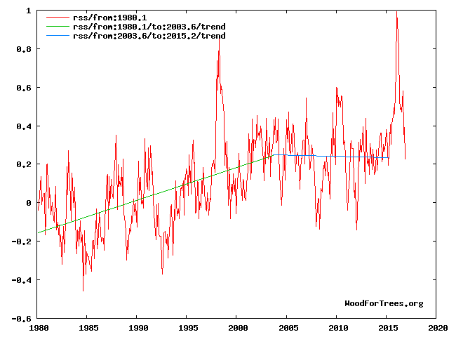
As to the sun climate relationship -the connection between solar “activity” and climate is poorly understood and highly controversial. Solar “activity” encompasses changes in solar magnetic field strength, IMF, GCRs, TSI, EUV, solar wind density and velocity, CMEs, proton events, etc. The idea of using the neutron count and the 10Be record as the most useful proxy for changing solar activity and temperature forecasting is agnostic as to the physical mechanisms involved. Having said that, however, it seems likely that the three main solar activity related climate drivers are the changing GCR flux – via the changes in cloud cover and natural aerosols (optical depth), the changing EUV radiation producing top down effects via the Ozone layer, and the changing TSI – especially on millennial and centennial scales. The effect on observed emergent behaviors i.e. global temperature trends of the combination of these solar drivers will vary non-linearly depending on the particular phases of the eccentricity, obliquity and precession orbital cycles at any particular time convolved with the phases of the millennial, centennial and decadal solar activity cycles and changes in the earth’s magnetic field. Because of the thermal inertia of the oceans there is a varying lag between the solar activity peak and the corresponding peak in the different climate metrics. There is a 13+/- year delay between the solar activity “Golden Spike” 1991 Oulu peak and the millennial cyclic “Golden Spike” temperature peak seen in the RSS data at 2003.6 . It has been independently estimated that there is about a 12-year lag between the cosmic ray flux and the temperature data – Fig. 3 in Usoskin (28).- in link above.
Fig 4. RSS trends showing the millennial cycle temperature peak at about 2003.6 (14)
The RSS cooling trend in Fig. 4 was truncated at 2015.3 because it makes no sense to start or end the analysis of a time series in the middle of major ENSO events which create ephemeral deviations from the longer term trends. By the end of August 2016, the strong El Nino temperature anomaly had declined rapidly. The cooling trend is likely to be fully restored by the end of 2019.
Anthony here is my prediction Leif is going to ruin your reputation.
[here is my prediction: I don’t give a damn what you think -take your petty personal war elsewhere – Anthony]
http://www.spaceweather.com/images2014/06dec14/missionduration_strip.gif
Figure 3.
Days in interplanetary space before a 30 year old astronaut reaches their career radiation limit for 3% risk of exposure-induced death (REID) at the 95% confidence level. Shown are maximum days before 3% REID limits are reached assuming different amounts of Al shielding (10 g/cm2 and 20 g/cm2). Black lines indicate times spanned by the Apollo missions from Apollo 8 (A8) to Apollo 17 (A17).
From Does the worsening galactic cosmic radiation environment observed by CRaTER preclude future manned deep space exploration?
For reasons that are well-known the GCR intensity is smaller at every even-odd sunspot minimum than at odd-even minima, so at the upcoming 24-25 cycle minimum, the GCR intensity will be lower than at the previous minimum, like this:
http://www.leif.org/research/GCR-Variation-Predicted.png
The Schwadron et al. prediction for a higher flux is simply wrong. Amazing that something like that can pass peer-review.
I recommend this fairly recent review paper by specialists in this field. You can skip most of the maths and still understand the paper.
Scherer, K., Fichtner, H., Borrmann, T., Beer, J., Desorgher, L., Flükiger, E., … & Heber, B. (2006). Interstellar-terrestrial relations: variable cosmic environments, the dynamic heliosphere, and their imprints on terrestrial archives and climate. Space Science Reviews, 127(1-4), 327-465.
https://tinyurl.com/y9zjwct8
Interesting.
This paper is consistent some others, namely, Evidence for a Global Warming at the Termination I Boundary and Its Possible Cosmic Dust Cause by LaViolette, INTRODUCTION: PALEOHELIOSPHERE VERSUS PALEOLISM by Frisch, and Frisch’s book, Solar Journey: The Significance of Our Galactic Environment for the Heliosphere and Earth.
However, in Figure 45 of the paper by Scherer et al., directly substitutes a Δ14C calibration curve as a 14C production curve, instead. The Δ14C calibration is not designed for use in papers directly, rather, the curve is used to determine the 14C production values of samples.
The authors may which to read The Technical Details: Determining Delta Values, Introduction to Radiocarbon Determination by the Accelerator Mass Spectrometry Method, and INTCAL09 AND MARINE09 RADIOCARBON AGE CALIBRATION CURVES 0–50,000 YEARS CAL BP
An illustrative application of IntCal09 is found in the paper 9,400 years of cosmic radiation and solar activity from ice cores and tree rings, esp. Fig. 2.
The latest calibration curve is IntCal13 with narrower results and a wider range of years.
Can’t see how this would affect the authors conclusions, made more robust by including 10Be.
Uh oh, link misspelled. Should be INTRODUCTION: PALEOHELIOSPHERE VERSUS PALEOLISM
And “which” should be “wish”
Another reasonably accessible paper.
Herbst, K., Kopp, A., Heber, B., Steinhilber, F., Fichtner, H., Scherer, K., & Matthiä, D. (2010). On the importance of the local interstellar spectrum for the solar modulation parameter. Journal of Geophysical Research: Atmospheres, 115(D1).
https://tinyurl.com/yad7fegk
Only one thing that totally controls ocean temperatures and any variation/deviation is down to ocean cycles and ocean circulation.
http://weather.unisys.com/archive/sst/sst-170611.gif
I’ve gained the impression that when the Sun is quiet EUV drops quite a lot but TSI only drops a little. I also get the idea that visible UV (I think that means UV A and UV B) increases quite a bit. If this is correct does it imply that the full frequency span of solar radiation shrinks somewhat when the Sun is quiet compared to when it is active?
If so could this result in less heating in the upper atmosphere when the Sun is quiet and a bigger proportion of TSI getting to the surface (relatively more energy entering the oceans and also reaching land surfaces) and might this lessen or maybe compensate for the reduction of TSI as seen at the Earth’s surface with a quiet Sun?
I’ve read that reduced EUV results in a thinning of the atmosphere in polar regions and causes the jet streams to wander. Coupled with relatively more energy going to the surface to fuel activity might this be responsible for phenomena like atmospheric rivers? Presumably during Solar maxima this might, because of the ocean’s damping effect, be less evident than during Solar minima when, on average, the Sun is more quiet.
I have been looking without success all over for a nice graph showing the Sun-spot numbers plotted over time together with EUV, visible UV and TSI as I think this might be useful.
I would appreciate some help with this.
This might be helpful:
http://www.leif.org/research/EUV-F107-and-TSI-CDR-HAO.pdf
There have been some comments that the sun’s magnetic field can’t greatly affect cosmic rays. Assuming that the same power law that describes the sun’s magnetic field at its surface and at earth’s orbit applies farther from the sun, some tracking I recently did shows that the sun’s field keeps cosmic rays below 1.26 * 10^11 GeV from reaching earth’s orbit. This of course applies on two axes; they aren’t shielded on the third axis.
A comment on the ice rafting graph in Svensmark’s book: I ran a Monte Carlo program to see what the probability is that the correlation is accidental. The answer is 1 in 16,000,000.
A comment on cloud formation: for the cosmic rays to have an effect, the relative humidity has to be in the right range. Too high, and clouds have already formed; too low, and they won’t form.
“…some tracking I recently did shows that the sun’s field keeps cosmic rays below 1.26 * 10^11 GeV…”
That’s 4/10ths the strength of the OMG particle!
” Too high, and clouds have already formed; too low, and they won’t form.”
Remember traveling by car near Rochester, MN one summer afternoon in 1972 and listening to the weather report on the radio. “Current temperature is 91 degrees with 90 percent relative humidity,” the announcer said.
Not a cloud in the sky.