Guest post by David Middleton
Introduction
When debating the merits of the CAGW (catastrophic anthropogenic global warming) hypothesis, I often encounter this sort of straw man fallacy:
All that stuff is a distraction. Disprove the science of the greenhouse effect. Win a nobel prize get a million bucks. Forget the models and look at the facts. Global temperatures are year after year reaching record temperatures. Or do you want to deny that.
This is akin to arguing that one would have to disprove convection in order to falsify plate tectonics or genetics in order to falsify evolution. Plate tectonics and evolution are extremely robust scientific theories which rely on a combination of empirical and correlative evidence. Neither theory can be directly tested through controlled experimentation. However, both theories have been tested through decades of observations. Subsequent observations have largely conformed to these theories.
Note: I will not engage in debates about the validity of the scientific theories of plate tectonics or evolution.
The power of such scientific theories is demonstrated through their predictive skill: Theories are predictive of subsequent observations. This is why a robust scientific theory is even more powerful than facts (AKA observations).
CAGW is a similar type of theory hypothesis. It relies on empirical (the “good”) and correlative evidence (the “bad”).
The Good
Carbon dioxide is a so-called “greenhouse” gas. It retards radiative cooling. All other factors held equal, increasing the atmospheric concentration of CO2 will lead to a somewhat higher atmospheric temperature. However, all other things are never held equal in Earth and Atmospheric Science… The atmosphere is not air in a jar; references to Arrhenius have no signficance.

Atmospheric CO2 has risen since the 19th century.

Humans are responsible for at least half of this rise in atmospheric CO2.

While anthropogenic sources are a tiny fraction of the total sources, we are removing carbon from geologic sequestration and returning it to the active carbon cycle.

The average temperature of Earth’s surface and troposphere has generally risen over the past 150 years.

Atmospheric CO2 has risen and warming has occurred.
The Bad
The modern warming began long before the recent rise in atmospheric CO2 and prior to the 19th century temperature and CO2 were decoupled:

The recent rise in temperature is no more anomalous than the Medieval Warm Period or the Little Ice Age:

Over the past 2,000 years, the average temperature of the Northern Hemisphere has exceeded natural variability (defined as two standard deviations from the pre-1865 mean) three times: 1) the peak of the Medieval Warm Period 2) the nadir of the Little Ice Age and 3) since 1998. Human activities clearly were not the cause of the first two deviations. 70% of the warming since the early 1600’s clearly falls within the range of natural variability.
While it is possible that the current warm period is about 0.2 °C warmer than the peak of the Medieval Warm Period, this could be due to the differing resolutions of the proxy reconstruction and instrumental data:

The amplitude of the reconstructed temperature variability on centennial time-scales exceeds 0.6°C. This reconstruction is the first to show a distinct Roman Warm Period c. AD 1-300, reaching up to the 1961-1990 mean temperature level, followed by the Dark Age Cold Period c. AD 300-800. The Medieval Warm Period is seen c. AD 800–1300 and the Little Ice Age is clearly visible c. AD 1300-1900, followed by a rapid temperature increase in the twentieth century. The highest average temperatures in the reconstruction are encountered in the mid to late tenth century and the lowest in the late seventeenth century. Decadal mean temperatures seem to have reached or exceeded the 1961-1990 mean temperature level during substantial parts of the Roman Warm Period and the Medieval Warm Period. The temperature of the last two decades, however, is possibly higher than during any previous time in the past two millennia, although this is only seen in the instrumental temperature data and not in the multi-proxy reconstruction itself.
[…]
The proxy reconstruction itself does not show such an unprecedented warming but we must consider that only a few records used in the reconstruction extend into the 1990s. Nevertheless, a very cautious interpretation of the level of warmth since AD 1990 compared to that of the peak warming during the Roman Warm Period and the Medieval Warm Period is strongly suggested.
[…]
The amplitude of the temperature variability on multi-decadal to centennial time-scales reconstructed here should presumably be considered to be the minimum of the true variability on those time-scales.
[…]

The climate of the Holocene has been characterized by a roughly millennial cycle of warming and cooling (for those who don’t like the word “cycle,” pretend that I typed “quasi-periodic fluctuation”):


These cycles (quasi-periodic fluctuations) even have names:

These cycles have been long recognized by Quaternary geologists:

Fourier analysis of the GISP2 ice core clearly demonstrates that the millennial scale climate cycle is the dominant signal in the Holocene (Davis & Bohling, 2001).

The industrial era climate has not changed in any manner inconsistent with the well-established natural millennial scale cycle. Assuming that the ice core CO2 is reliable, the modern rise in CO2 has had little, if any effect on climate.
The Null Hypothesis
What is a ‘Null Hypothesis’
A null hypothesis is a type of hypothesis used in statistics that proposes that no statistical significance exists in a set of given observations. The null hypothesis attempts to show that no variation exists between variables or that a single variable is no different than its mean. It is presumed to be true until statistical evidence nullifies it for an alternative hypothesis.
Read more: Null Hypothesis http://www.investopedia.com/terms/n/null_hypothesis.asp#ixzz4eWXO8w00
Follow us: Investopedia on Facebook
Since it is impossible to run a controlled experiment on Earth’s climate (there is no control planet), the only way to “test” the CAGW hypothesis is through models. If the CAGW hypothesis is valid, the models should demonstrate predictive skill. The models have utterly failed:


The models have failed because they result in a climate sensitivity that is 2-3 times that supported by observations:

From Hansen et al. 1988 through every IPCC assessment report, the observed temperatures have consistently tracked the strong mitigation scenarios in which the rise in atmospheric CO2 has been slowed and/or halted.
Apart from the strong El Niño events of 1998 and 2015-16, GISTEMP has tracked Scenario C, in which CO2 levels stopped rising in 2000, holding at 368 ppm.

The utter failure of this model is most apparent on the more climate-relevant 5-yr running mean:

This is from IPCC’s First Assessment Report:

HadCRUT4 has tracked below Scenario D.

This is from the IPCC’s Third Assessment Report (TAR):

HadCRUT4 has tracked the strong mitigation scenarios, despite a general lack of mitigation.
The climate models have never demonstrated any predictive skill.
And the models aren’t getting better. Even when they start the model run in 2006, the observed temperatures consistently track at or below the low end 5-95% range. Observed temperatures only approach the model mean (P50) in 2006, 2015 and 2016.

The ensemble consists of 138 model runs using a range of representative concentration pathways (RCP), from a worst case scenario RCP 8.5, often referred to as “business as usual,” to varying grades of mitigation scenarios (RCP 2.6, 4.5 and 6.0).

When we drill wells, we run probability distributions to estimate the oil and gas reserves we will add if the well is successful. The model inputs consist of a range of estimates of reservoir thickness, area and petrophysical characteristics. The model output consists of a probability distribution from P10 to P90.
- P10 = Maximum Case. There is a 10% probability that the well will produce at least this much oil and/or gas.
- P50 = Mean Case. There is a 50% probability that the well will produce at least this much oil and/or gas. Probable reserves are >P50.
- P90 = Minimum Case. There is a 90% probability that the well will produce at least this much oil and/or gas. Proved reserves are P90.
Over time, a drilling program should track near P50. If your drilling results track close to P10 or P90, your model input is seriously flawed.
If the CMIP5 model ensemble had predictive skill, the observations should track around P50, half the runs should predict more warming and half less than is actually observed. During the predictive run of the model, HadCRUT4.5 has not *tracked* anywhere near P50…

I “eyeballed” the instrumental observations to estimate a probability distribution of predictive run of the model.
Prediction Run Approximate Distribution
2006 P60 (60% of the models predicted a warmer temperature)
2007 P75
2008 P95
2009 P80
2010 P70
2011-2013 >P95
2014 P90
2015-2016 P55
Note that during the 1998-99 El Niño, the observations spiked above P05 (less than 5% of the models predicted this). During the 2015-16 El Niño, HadCRUT only spiked to P55. El Niño events are not P50 conditions. Strong El Niño and La Niña events should spike toward the P05 and P95 boundaries.
The temperature observations are clearly tracking much closer to strong mitigation scenarios rather than RCP 8.5, the bogus “business as usual” scenario.
The red hachured trapezoid indicates that HadCRUT4.5 will continue to track between less than P100 and P50. This is indicative of a miserable failure of the models and a pretty good clue that the models need be adjusted downward.
In any other field of science CAGW would be a long-discarded falsified hypothesis.
Conclusion
Claims that AGW or CAGW have earned an exemption from the Null Hypothesis principle are patently ridiculous.
In science, a broad, natural explanation for a wide range of phenomena. Theories are concise, coherent, systematic, predictive, and broadly applicable, often integrating and generalizing many hypotheses. Theories accepted by the scientific community are generally strongly supported by many different lines of evidence-but even theories may be modified or overturned if warranted by new evidence and perspectives.
This is not a scientific hypothesis:
More CO2 will cause some warming.
It is arm waving.
This is a scientific hypothesis:
A doubling of atmospheric CO2 will cause the lower troposphere to warm by ___ °C.
Thirty-plus years of failed climate models never been able to fill in the blank. The IPCC’s Fifth Assessment Report essentially stated that it was no longer necessary to fill in the blank.
While it is very likely that human activities are the cause of at least some of the warming over the past 150 years, there is no robust statistical correlation. The failure of the climate models clearly demonstrates that the null hypothesis still holds true for atmospheric CO2 and temperature.
Selected References
Davis, J. C., and G. C. Bohling, The search for patterns in ice-core temperature curves, 2001, in L. C. Gerhard, W. E. Harrison, and B. M. Hanson, eds., Geological perspectives of global climate change, p. 213–229.
Finsinger, W. and F. Wagner-Cremer. Stomatal-based inference models for reconstruction of atmospheric CO2 concentration: a method assessment using a calibration and validation approach. The Holocene 19,5 (2009) pp. 757–764
Grosjean, M., Suter, P. J., Trachsel, M. and Wanner, H. 2007. Ice-borne prehistoric finds in the Swiss Alps reflect Holocene glacier fluctuations. J. Quaternary Sci.,Vol. 22 pp. 203–207. ISSN 0267-8179.
Hansen, J., I. Fung, A. Lacis, D. Rind, Lebedeff, R. Ruedy, G. Russell, and P. Stone, 1988: Global climate changes as forecast by Goddard Institute for Space Studies three-dimensional model. J. Geophys. Res., 93, 9341-9364, doi:10.1029/88JD00231.
Kouwenberg, LLR, Wagner F, Kurschner WM, Visscher H (2005) Atmospheric CO2 fluctuations during the last millennium reconstructed by stomatal frequency analysis of Tsuga heterophylla needles. Geology 33:33–36
Ljungqvist, F.C. 2009. N. Hemisphere Extra-Tropics 2,000yr Decadal Temperature Reconstruction. IGBP PAGES/World Data Center for Paleoclimatology Data Contribution Series # 2010-089. NOAA/NCDC Paleoclimatology Program, Boulder CO, USA.
Ljungqvist, F.C. 2010. A new reconstruction of temperature variability in the extra-tropical Northern Hemisphere during the last two millennia. Geografiska Annaler: Physical Geography, Vol. 92 A(3), pp. 339-351, September 2010. DOI: 10.1111/j.1468-459.2010.00399.x
MacFarling Meure, C., D. Etheridge, C. Trudinger, P. Steele, R. Langenfelds, T. van Ommen, A. Smith, and J. Elkins. 2006. The Law Dome CO2, CH4 and N2O Ice Core Records Extended to 2000 years BP. Geophysical Research Letters, Vol. 33, No. 14, L14810 10.1029/2006GL026152.
Moberg, A., D.M. Sonechkin, K. Holmgren, N.M. Datsenko and W. Karlén. 2005. Highly variable Northern Hemisphere temperatures reconstructed from low-and high-resolution proxy data. Nature, Vol. 433, No. 7026, pp. 613-617, 10 February 2005.
Instrumental Temperature Data from Hadley Centre / UEA CRU, NASA Goddard Institute for Space Studies and Berkeley Earth Surface Temperature Project via Wood for Trees.
A fine article. But I think you missed an opportunity to introduce an even more basic argument.
The accepted theory (for the most part by both sides) is that doubling of CO2 has a direct effect equivalent to 3.7 w/m2. This translates into just over 1 degree of warming (sans feedbacks). That needs to be put into the context of our current timeline which can be directly confirmed by direct observations, namely that:
o We are currently at ~ 400 ppm
o CO2 concentration is increasing at ~ 2 ppm per year
That means, to experience just one degree of direct warming from CO2 increases will take two hundred years. To get to two degrees of direct warming from CO2 at present rates of increase would take six hundred years.
Of course there are feedbacks which are controversial. But if they were large, they would be easily observable in the current data. They aren’t. If they exist at all they are swamped by natural variability. So, we are left with a problem that based on both theory and observable data is not only small, but moving so slowly that it will take centuries to appear in any meaningful fashion. All the rest is hype.
CO2 is logarithmic. The catastrophe argument should have died on that fact alone.
A correlation of the high resolution DE08 ice core and Moberg’s reconstruction yields a climate sensitivity of 1.5 to 2.0 °C.
http://i90.photobucket.com/albums/k247/dhm1353/LawMob3.png
However, this assumes that all of the warming since 1830 was driven by CO2… At least half of that warming was clearly not related to CO2.
David, I think although admittedly well-argued, your article ignores some well-established science that climate change will lead to 1) higher beer prices http://www.citizen-times.com/story/news/politics/elections/2016/01/27/noaa-global-warming-may-affect-your-beer-and-its-price/79400280/ , 2) more hookers http://dailycaller.com/2013/04/30/democrats-global-warming-means-more-hookers/ , and mutant frogs https://wattsupwiththat.com/2012/10/25/now-its-the-frogs-affected-by-climate-change-again/ — I could go on…
I gave up beer for bourbon and red wine a long time ago.
More hookers and mutant frogs could be a problem in some neighborhoods.
David,
Scotch might have fewer calories, given bourbon’s sweetness and derivation from corn rather than barley. That’s not why I prefer it, but it might become and excuse.
If the mutant frogs have larger legs, I’m all for them.
If the hookers stay off the streets and indoors cooking frogs’ legs and taking antibiotics, the problem is greatly reduced.
Chimp, be careful hat you wish for !!
 &sp=5163d006c945bf2f3c45fb19a1fda082
The population dynamics of Adélie and emperor penguins are strongly influenced by the Antarctic environment and climatic variation. Based on the heterozygous sites identified in the penguin genomes, we used the pairwise sequentially Markovian coalescent (PSMC) method [30] to infer fluctuations in the effective population sizes of the two penguins from 10 MYA to 10 thousand years ago (KYA). From 10 MYA to 1 MYA, both species had relatively small and stable effective population sizes of <100,000, and the populations expanded gradually from ∼1 MYA (Figure 1B). The effective population size of the Adélie penguin appears to have increased rapidly after ∼150 KYA, at a time when the penultimate glaciation period ended and the climate became warmer. This expansion is consistent with the prediction in a previous study based on mitochondrial data from two Adélie penguin lineages [31] and with the recent observations that Adélie populations expanded when more ice-free locations for nesting became available [32]. Notably, at ∼60 KYA, within a relatively cold and dry period called Marine Isotope Stage 4 (MIS4) [33] in the last glacial period, the effective population size of Adélie penguins declined by ∼40% (Figure 1B and C). By contrast, the effective population size of emperor penguin remained at a stable level during the same period.
https://academic.oup.com/gigascience/article-lookup/doi/10.1186/2047-217X-3-27
Climate is controlled by natural cycles. Earth is just past the 2004+/- peak of a millennial cycle and the current cooling trend will likely continue until the next Little Ice Age minimum at about 2650.See the Energy and Environment paper at http://journals.sagepub.com/doi/full/10.1177/0958305X16686488
and an earlier accessible blog version at http://climatesense-norpag.blogspot.com/2017/02/the-coming-cooling-usefully-accurate_17.html
Here is the abstract for convenience :
“ABSTRACT
This paper argues that the methods used by the establishment climate science community are not fit for purpose and that a new forecasting paradigm should be adopted. Earth’s climate is the result of resonances and beats between various quasi-cyclic processes of varying wavelengths. It is not possible to forecast the future unless we have a good understanding of where the earth is in time in relation to the current phases of those different interacting natural quasi periodicities. Evidence is presented specifying the timing and amplitude of the natural 60+/- year and, more importantly, 1,000 year periodicities (observed emergent behaviors) that are so obvious in the temperature record. Data related to the solar climate driver is discussed and the solar cycle 22 low in the neutron count (high solar activity) in 1991 is identified as a solar activity millennial peak and correlated with the millennial peak -inversion point – in the RSS temperature trend in about 2004. The cyclic trends are projected forward and predict a probable general temperature decline in the coming decades and centuries. Estimates of the timing and amplitude of the coming cooling are made. If the real climate outcomes follow a trend which approaches the near term forecasts of this working hypothesis, the divergence between the IPCC forecasts and those projected by this paper will be so large by 2021 as to make the current, supposedly actionable, level of confidence in the IPCC forecasts untenable.””
Here is another excerpt from the paper;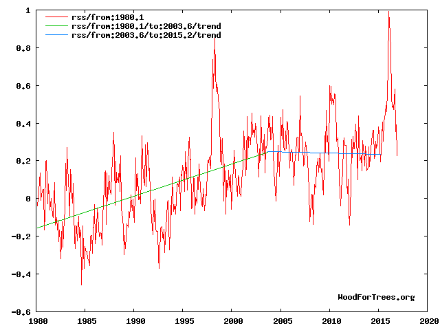
Any discussion or forecast of future cooling must be based on a wide knowledge of the most important reconstructions of past temperatures, after all, the hockey stick was instrumental in selling the CAGW meme to the grant awarders, politicians, NGOs and the general public.
The following papers trace the progressive development of the most relevant reconstructions starting with the hockey stick: Mann et al 1999. Fig. 3 (10), Esper et al 2002 Fig. 3 (11), Mann’s later changes – Mann et al 2008 Fig. 3 (12), and Mann et al 2009 Fig. 1 (13). The later 2012 Christiansen and Ljungqvist temperature time series of Fig. 3 is here proposed as the most useful “type reconstruction” as a basis for climate change discussion. For real world local climate impact estimates, Fig 3 shows that the extremes of variability or the data envelopes are of more significance than averages. Note also that the overall curve is not a simple sine curve. The down trend is about 650 years and the uptrend about 364 years. Forward projections made by mathematical curve fitting have no necessary connection to reality, particularly if turning points picked from empirical data are ignored.
Figure 4 illustrates the working hypothesis that for this RSS time series the peak of the Millennial cycle, a very important “golden spike”, can be designated at 2003.6
The RSS cooling trend in Fig. 4 and the Hadcrut4gl cooling in Fig. 5 were truncated at 2015.3 and 2014.2, respectively, because it makes no sense to start or end the analysis of a time series in the middle of major ENSO events which create ephemeral deviations from the longer term trends. By the end of August 2016, the strong El Nino temperature anomaly had declined rapidly. The cooling trend is likely to be fully restored by the end of 2019.
From Figures 3 and 4 the period of the latest Millennial cycle is from 990 to 2004 – 1,014 years. This is remarkably consistent with the 1,024-year periodicity seen in the solar activity wavelet analysis in Fig. 4 from Steinhilber et al 2012 (16).
A very good review of solid points. I question only one and not for its effect on the bottom line of your work.
“Humans are responsible for at least half of this rise in atmospheric CO2.”
If Salby, Humlum, Harde, and Hertzberg are right Our CO2 is not even controlling atmospheric content and the net AGW due to CO2 has to be small enough to make it indecipherable from the noise in the measurements. With CO2 following the integral of temperature (Salby) and temperature leading CO2 on short time scales (Humlum) I find the model based attribution statements of over 50% unconvincing. The IPCC position that all the increase in CO2 since the industrial age is from anthropogenic causes is not based on very convincing evidence. A very small variation in natural carbon sinks could completely mask the fossil fuel source.
I think that attribution studies need,at a minimum, to seriously consider these claims and a realistic and thorough analysis of the carbon cycle. For starters the residence time of CO2 from the nuclear test ban treaty is less than 10 years not 200 as used in the Bern model.
Atmospheric residence time is short. On the order of 5-10 years. However, the residence time of individual CO2 molecules isn’t very relevant. The “e-folding” time is what matters. We have been taking carbon out of geologic sequestration (coal, oil, natural gas) and putting it back into the active carbon cycle (atmosphere, oceans, soil, biosphere). It takes many decades to hundreds of years for the carbon to return to geologic sequestration (lime muds, etc.).
The geological sequestration time of 100y+ is not relevant. At the instant any single atom of carbon is taken out of the atmosphere by an animal or plant and sequestered into the structure of the plant then that atom of carbon is “off the list” with respect to any effect on the atmosphere. So what is relevant is the planet wide daily plant and animal extraction of atmospheric CO2. There will be some loss back to the atmosphere in plant/animal decay but a good proportion that has been “stuck” in the organic structures will stay there for a very long time. A careful study of the biosphere part of the carbon cycle might enable us to put some numbers on this. Keep remembering though it is not the moment that the carbon atom becomes coal/oil that is important but the moment the atom is “sucked” out of the atmosphere initially.
Your “e-folding” time is observed directly from the 14CO2 time curve starting at the 1963 atomic test ban treaty. The bomb 14CO2 was the pulse, and is measured very accurately in both hemispheres.
The 14CO2 of the atmosphere declined by one-half from the peak in 1964 to 1974.
That means that all atmospheric CO2 is removed to “permanent” geological sinks very rapidly.
This 10 year period is equivalent to a “tau” or “e-folding” time of 16 years. That is not a calculation, it is an observed fact.
CO2 never accumulates in the atmosphere on any time scale, from any source. Atmospheric CO2 is a transient stream from very deep sources to very deep sinks. Oceans, biological and geological.
And science still doesn’t know what all the sinks are or might be.
CAGW is anti-science, in the same class with ID, if not quite YE creationism. Yet.
But give them time. When earth starts dramatically cooling again, as in the ’40s, ’50s, ’60s and ’70s, despite rising CO2, then we’ll probably see lying of biblical proportions.
I wouldn’t classify GAGW as quite that bad… But it’s close.
David,
I’ll grant that CAGW is more science-y than YEC, but it’s still contrary to the scientific method.
That is the thrust of this thread.
For which I and so many others thank you.
@BW,
14C isn’t a stable isotope.
DMA,
And the OCO-2 satellite maps don’t make a compelling argument that the urban areas are the major source of CO2. It seems that the CO2 is largely biogenic and from outgassing in the tropical seas.
Outgassing is, by far, the largest source… As big as all the other sources combined… About 20 times that of anthropogenic emissions.
The difference is that we are taking a tiny bit of carbon out of geologic sequestration every year and putting it back into the active carbon cycle.
Clyde
If you check out Ole Humlum’s web site, http://www.climate4you.com/, you see in depth analysis of the CO2 variation over time with respect to temperature. He has demonstrated a clear lag and categorically states the atmospheric CO2 is “(6) CO2 released from anthropogene sources apparently has little influence
on the observed changes in atmospheric CO2, and
changes in atmospheric CO2 are not tracking changes in human
emissions.”
This aligns with Salby’s work and further reduces the acceptability of AGW along with the other valid points made in this article.
David,
You said, “The difference is that we are taking a tiny bit of carbon out of geologic sequestration every year and putting it back into the active carbon cycle.” I’m well aware that humans are accelerating the rate at which CO2 is produced from geologic materials such as fossil fuels and limestone.
However, the point is that, as you yourself remarked, these physical processes don’t proceed in a bottle in a laboratory. In the real world, there are numerous interactions — feedbacks — that control the overall impact.
As Robert of Ottawa has already observed, when humans produce CO2 one of the consequences is to increase the partial pressure of CO2 at the surface of the ocean, thereby reducing the diffusion rate of outgassing CO2. Therefore, humans may be shifting the location and magnitude of the sources and sinks, but not so much changing the balance. It matters not where the CO2 comes from, it matters only if humans are truly increasing the amount above what would be expected in a warming world. If the world is warming for other reasons, then one would expect outgassing to increase CO2 coincidentally with human production of it.
The AGW theory predicts that most of the warming should occur at night and in the Winter. However, in recent years, the diurnal highs have been increasing faster than the lows. That would appear to be a different process controlling that, but it would explain an increase in atmospheric CO2.
Cooling at night is regulated by water vapor to dew point temperature. Dew points went up when the amo cycle in 2000 positive, as well as the various positive pdo’s the last 20 years.
Min temp follows dew point.
micro6500,
I agree that dew point (and clouds) will impact night-time cooling. However, it is central to the AGW theory that CO2 plays a similar role.
Which is why it is wrong.
the partial pressure of CO2
===========
at the partial pressure of CO2 increases, it becomes harder for water to evaporate, reducing the amount of water in the atmosphere.
I have no quarrel with that part of the analysis. But I can’t find any error in Salbys carbon flux analysis and think that minor natural variations in CO2 sources and sinks, each 30 to 50 times the volume of anthropogenic sources, could just as easily explain the recent rise. If A CO2 was the only source of the rise why , in 2002 when it changed rate by a factor of 3 did the rate of change of atmospheric CO2 not change. Same for the last 3 years when A CO2 flattened out but had no measurable effect on rate of rise in the atmosphere. It is almost like we are saying the fossil fuel emission rate controls the natural sink rate in order to keep the growth in the atmosphere steady.
The sink rate has varied with the emissions. It actually appears to be increasing over time:
http://i90.photobucket.com/albums/k247/dhm1353/Law1600.png
During the mid-20th century cooling, the sink rate increased and “consumed” more than a decade’s worth of CO2 emissions.
http://i90.photobucket.com/albums/k247/dhm1353/Law19301970.png
https://wattsupwiththat.com/2012/12/07/a-brief-history-of-atmospheric-carbon-dioxide-record-breaking/
David M.
Salby shows that sink rate is a function of atmospheric CO2 content. It will rise as CO2 increases but is sensitive only to content not source. If the rise in CO2 is mostly natural the change of sink rate is mostly natural. The anthropogenic portion is proportional to the ratio of anthropogenic to natural atmospheric content. This calculation is where the residence time is important.
The CO2 sink rate should vary as a percentage of total CO2, because the sink cannot distinguish between human and natural CO2. But instead the sink rate remains a percentage of the increase in human emissions.
this suggests the CO2 sink is not a sink at all.
Fred, the amount of co2 that is missing from the official sources is enormous. From 1998 till now all of the co2 produced above the 1998 level is gone. The sinking is the base plus. This when 38 % of all anthropogenic co2 has been produced. If this rate continues, even with production, the co2 ppm per year will become negative. I am really surprised that 2016 came in at 3 ppm. It should have been 5 at the very least. I would have been ok at 4, but not 3.
Abstract
Environmental change drives demographic and evolutionary processes that determine diversity within and among species. Tracking these processes during periods of change reveals mechanisms for the establishment of populations and provides predictive data on response to potential future impacts, including those caused by anthropogenic climate change. Here we show how a highly mobile marine species responded to the gain and loss of new breeding habitat. Southern elephant seal, Mirounga leonina, remains were found along the Victoria Land Coast (VLC) in the Ross Sea, Antarctica, 2,500 km from the nearest extant breeding site on Macquarie Island (MQ). This habitat was released after retreat of the grounded ice sheet in the Ross Sea Embayment 7,500–8,000 cal YBP, and is within the range of modern foraging excursions from the MQ colony. Using ancient mtDNA and coalescent models, we tracked the population dynamics of the now extinct VLC colony and the connectivity between this and extant breeding sites. We found a clear expansion signal in the VLC population ∼8,000 YBP, followed by directional migration away from VLC and the loss of diversity at ∼1,000 YBP, when sea ice is thought to have expanded. Our data suggest that VLC seals came initially from MQ and that some returned there once the VLC habitat was lost, ∼7,000 years later. We track the founder-extinction dynamics of a population from inception to extinction in the context of Holocene climate change and present evidence that an unexpectedly diverse, differentiated breeding population was founded from a distant source population soon after habitat became available.
http://journals.plos.org/plosgenetics/article?id=10.1371/journal.pgen.1000554
David, you write:
No. It is pretty easy to test the validity of the AGW conjecture (it is not an hypothesis, it is mere speculation) against real-world data. All you need to know is what the idea of “global warming” as an effect of a so-called “enhanced GHE” is actually claiming as its “warming mechanism”. Here it is:
http://www.climatetheory.net/wp-content/uploads/2012/05/greenhouse-effect-held-soden-2000.png
The postulated “greenhouse warming mechanism” is a very specific one. It is the one about the “raised ERL” (Effective Radiating Level) of the Earth, Z_e in the figure above. In the words of Raymond T. Pierrehumbert:
https://geosci.uchicago.edu/~rtp1/papers/PhysTodayRT2011.pdf
“An atmospheric greenhouse gas enables a planet to radiate at a temperature lower than the ground’s, if there is cold air aloft. It therefore causes the surface temperature in balance with a given amount of absorbed solar radiation to be higher than would be the case if the atmosphere were transparent to IR. Adding more greenhouse gas to the atmosphere makes higher, more tenuous, formerly transparent portions of the atmosphere opaque to IR and thus increases the difference between the ground temperature and the radiating temperature. The result, once the system comes into equilibrium, is surface warming.”
What we want to look for, then, is the following:
Over time, T_s (and T_tropo) should be observed to go up while the T_e should either be observed to stay flat, or at least follow a significantly lower trend than the T_s/T_tropo.
We can track T_s and T_tropo over time, but how do we keep track of T_e? Well, T_e is directly associated with Earth’s average emission flux to space, that is the OLR at the ToA. T_e is, after all, not a real temperature, it is rather Earth’s average emission flux to space expressed as a temperature, via the Stefan-Boltzmann equation. Earth’s OLR to space (basically, its planetary heat loss (Q_out)) very nearly balances the average incoming heat flux from the Sun (Q_in), the ASR (TSI minus refl SW (albedo)), which is ~239 W/m^2.
239 W/m^2 translate into a T_e of 255K. So if T_e stays the same over time, it means that the OLR stays flat also. Or, if there is warming caused by other processes, such as increased solar heating, the OLR will be observed to go up, but we will still expect it to rise LESS over time than the corresponding surface and tropospheric temps. Actually, tropospheric temps (T_tropo) are a better gauge in this regard than surface temps (T_s), since ~85% of Earth’s outgoing long-wave radiation through the ToA to space originates from the troposphere, which means that the OLR flux is chiefly tied – at least over time – simply to the average tropospheric temperature.
Why exactly do we expect the OLR to rise less than the corresponding T_tropo over time? Refer again to the Held/Soden schematic above, plus take in what Pierrehumbert is saying here (same link as above):
“The greenhouse effect shifts [Earth’s] surface temperature toward the [Sun’s] photospheric temperature by reducing the rate at which the planet loses energy at a given surface temperature. The way that works is really no different from the way adding fiberglass insulation or low-emissivity windows to your home increases its temperature without requiring more energy input from the furnace. The temperature of your house is intermediate between the temperature of the flame in your furnace and the temperature of the outdoors, and adding insulation shifts it toward the former by reducing the rate at which the house loses energy to the outdoors.”
THAT’S the postulated “greenhouse warming mechanism” right there. At a given T_s (and T_tropo), making the atmosphere more opaque to outgoing surface IR, will REDUCE its heat loss to space (that’s the OLR at the ToA). And so, in order for the OLR to NOT reduce, but rather stay the same, still in balance with the heat input from the Sun, the T_s/T_tropo needs to RISE, because higher temps means more thermal radiation (IR) is emitted. That way, over time, T_s/T_tropo would be observed to rise gradually, while T_e (OLR) would stay quite unchanged. That’s the so-called “radiative forcing” in theoretical operation.
However, is this something we see in the real Earth system? Can we find this AGW signal anywhere?
The simple answer is: Nope. Everything seems to be working EXACTLY the way one would expect if there weren’t an “enhancement” of some “GHE” going on in the Earth system. The OLR at the ToA has simply gone up in step with the T_tropo over the last 32+ years, according to the available ToA radiation flux data (ERBS Ed3_Rev1+CERES EBAF Ed4, corroborated by HIRS and ISCCP FD):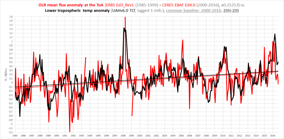
A controlled experiment would require two planet Earth’s. One planet would be subjected to an increase in atmospheric CO2 and the second Earth would be the “control” planet and not subjected to an increase in atmospheric CO2.
David,
I’m not sure I understand your position.
Our one planet HAS been “subjected to an increase in atmospheric CO2” over the last decades, and there are definite predictions made by the “enhanced GHE hypothesis” as to what we would expect to observe in the Earth system given such an increase. These are predictions we can test directly against the actual available observational data from the REAL Earth system.
Over the last 32 years, the total atmospheric content of CO2 increased by 17%, or about half (!!) of the entire rise since pre-industrial times. To make matters worse, during the same period of time, the total tropospheric content of water vapour (TPW) also increased substantially, by at least 1.5kg on average on top of each m^2 of surface (or about 5%).
This rather consistent and, quite frankly, remarkable rise (since 1985) in the overall atmospheric concentration of IR-active gases, so-called “GHGs”, should – in theory – have strengthened the so-called “greenhouse effect” immensely, by reducing earth’s radiative heat loss to space at any given (altitude-specific) temperature through the raising of our planet’s ERL (“effective radiating level”) to space, and thus constitute a clear cause of warming.
However, we do not observe ANY systematic reduction in OLR relative to tropospheric temps from 1985 to 2016. There is no trace of any “enhanced GHE”, theoretically assumed to be caused by the considerable increase in atmospheric “GHG” concentration, anywhere in the real-world radiation flux data. The OLR is simply found to track tropospheric temps over time, the latter clearly the cause and the former a mere effect.
And so there is an obvious problem with the ‘theory’ … It does not match the real-world observations. The warming is clearly natural. And we know (again from the real-world data) what did it. The Sun:


(ToA solar heat in (Q_in(SW), TSI minus refl SW (albedo).)
(ToA Earth heat loss to space (Q_out(LW)).)
(ToA net flux (Q_in(SW) minus Q_out(LW)).)
Our current positive radiative (heat) balance at the ToA is caused in full by an increase in Q_in(SW) and rather countered somewhat by a simultaneous increase in Q_out(LW), the obvious causal chain being:
+ASR => +T => +OLR
As we know that a 2 planet experiment is currently impractical (Magrathean delivery time too long) we have no choice but to look at the one we have got. So Kristian has exactly the right idea, look for an AGW/CO2 radiative forcing “signal” in something we can observe/measure. I do like the T-s/T-tropo consideration but for some reason at the back of my mind I feel we need to have a bit of a handle on the time constant involved here. How long, for a specific CO2 concentration, do we have to wait for the earth to heat up and restore the effective temperature i.e. get the outgoing radiation to space back up to the figure to match incoming? Not sure I have seen this time constant discussed on either side of the debate but I get the feeling the AGW crowd think this is a thing that happens over years. I suspect it is massively shorter, the red and black curves in Kristians graph match so well it suggests very little time lag and from experience the heating/cooling of land and oceans over the seasons seems pretty rapid too (otherwise you wouldn’t see different seasonal temperatures).
The Badger, you ask:
According to the “enhanced GHE hypothesis” and its “raised ERL” warming mechanism, there is no discernible time lag between “forcing” and “temp rise”. That is precisely why we do not expect to see a reduction in OLR (T_e) over time. It is supposed to stay – observably – constant while the T_s/T_tropo rises.
This is what people tend to “forget”. In the real world, the slow, gradual increase in atmospheric CO2 is specifically NOT supposed to result in a reduction in OLR over time, because it is all supposed to happen incrementally, and so as the extra increment of CO2 input reduces the outgoing IR a tiny bit, the temperature is rather at once forced to rise a tiny bit, and by that letting the Earth system rid itself of the energy that was initially held back, RESTORING THE HEAT BALANCE at each incremental step. The next increment of CO2 input arrives, forcing T to rise a tiny bit more, restoring the balance once again. And so on and so forth. What we will OBSERVE over time, then, is simply a stable radiative balance at the ToA (SW in = LW out) with NO net accumulation of energy inside the Earth system as a whole, but with steadily rising Earth system temperatures at each altitude-specific level (from sfc to tropopause) all the same. How is this? Earth’s “effective radiating level” (ERL) is raised, not in giant leaps (as if the atmospheric CO2 content were doubled overnight), but slowly and gradually over time, maintaining a constant Earth T_e to space, but forcing the T_s to rise (via the lapse rate). THAT’S the postulated “greenhouse” warming mechanism, after all:
http://www.climatetheory.net/wp-content/uploads/2012/05/greenhouse-effect-held-soden-2000.png
And so, observing a positive radiation imbalance at the ToA is specifically NOT a sign of an “enhanced GHE”, but of something else. And this “something else” is of course – as the ToA radiation flux data shows us – an increase in ASR (“absorbed solar radiation”), the solar heat input to the Earth system.
Law Dome CO2 vs instrumental records
The Law Dome CO2 is low pass filtered by diffusion and compression averaging out decades or more.
In contrast, the Keeling CO2 data is not. NOAA patches Law Dome to Keeling curve – to give a misleading apples/oranges curve implying very rapid recent rise vs slow ancient changes – when all fast paleo changes were filtered off.
The DE08 core at Law Dome actually has a fairly high resolution, possibly as good as 10 years.
So, as long as the Keeling curve is filtered with at least a 10-yr average, it can be directly compared to the DE08 core.
Now, the older, deeper cores, with record lengths clearly should never be spliced onto the instrumental data or the DE08 core.
https://wattsupwiththat.com/2017/03/28/breaking-hockey-sticks-antarctic-ice-core-edition/
David Middleton While you can see 10 yr resolution – there is still diffusion smoothing out the variations.
The delta between the ice and gas ages is 30 years in the DE08 core. At the very worst, the smoothing is 30 years. Firn densification models suggest that the smoothing could be on the order of 10 years. MacFarling-Meure present the data as a 20-yr spline fit.
It’s really difficult to pin down exactly what the gas resolution is.
without correlation you simply cannot have causation … period, full stop … 1940 – 1970 … CO2 Up, Temperature Flat or Down … no correlation … CO2 (alone) cannot be causation of rising temperatures …
There is some correlation over longer periods of time. The DE08 core (red curve) exhibits a fair correlation since 1830:
http://i90.photobucket.com/albums/k247/dhm1353/LawMob2.png
However, the natural variability of temperature changes dwarfs the CO2 effect.
And the high resolution DE08 ice core actually indicates a pause or possible drop in atmospheric CO2 in the 1940’s and 1950’s.
https://wattsupwiththat.com/2012/12/07/a-brief-history-of-atmospheric-carbon-dioxide-record-breaking/
http://i90.photobucket.com/albums/k247/dhm1353/Law19301970.png
The R squared value of 0.32 shown in your graph is way to low to indicate any possible correlation between CO2 concentration and temperature anomaly.
0.32 is actually a fairly strong R-squared. About 1/3 of the observations fit the trend. This would imply that up to 1/3 of the warming since 1830 could be related to the rise in CO2.
I was studying the ACS Climate Change tool kit sections on the single and multilayer theories (what I refer to as the thermal ping-pong ball) of upwelling/downwelling/”back” radiation and after seeing a similar discussion on an MIT online course (specifically says no transmission) have some observations.
These layered models make no reference to conduction, convection or latent heat processes which leads me to conclude that these models include no molecules, aka a “non-participating media,” aka vacuum. This is a primary conditional for proper application of the S-B BB ideal, i.e. ε = 1.0, equation.
When energy strikes an object or surface there are three possible results: reflection or ρ, absorption or α, transmission or τ and ρ + α + τ = 1.0.
The layered models use only α which according to Kirchhoff is equal to ε. What Kirchhoff really means is that max emissivity can equal but not exceed the energy absorbed. Nothing says emissivity can’t be less that the energy absorbed. If α leaves as conduction/convection/latent (net macro floes, non-thermodynamic equilibrium) than ε will be much less than 1.0.
These grey bodied layered models then exist in a vacuum and are 100% non-reflective, i.e. opaque, surfaces, i.e. just like the atmosphere. NOT!
So the real atmosphere has real molecules meaning a “participatory” media and is 99.96% transparent i.e. non-opaque.
Because of the heat flow participating molecules only 63 W/m^2 of the 160 W/m^2 that made it to the surface leave the surface as LWIR. (K-T Figure 10)
63 W/m^2 and 15 C / 288 K surface gives a net effective ε of about 0.16 when the participating media is considered. (BTW “surface” is NOT the ground, but 1.5 m ABOVE the ground per WMO & IPCC AR5 glossary.)
So the K-T diagram is thermodynamic rubbish, earth as a ball in a bucket of hot mush is physical rubbish, the Δ 33 C w/ atmosphere is obvious rubbish, the layered models are unrelated to reality rubbish, the ground losing 396 W/m^2 is rubbish.
The atmosphere is not in thermodynamic equilibrium and as a consequence neither Stephan Boltzmann nor Kirchhoff can be a used the ways the GHE theory applies them.
What support does the GHE theory have left besides rabid minions?
I see no reason why GHE theory gets a free pass on the scientific method.
https://www.acs.org/content/acs/en/climatescience/atmosphericwarming.html
http://web.mit.edu/16.unified/www/FALL/thermodynamics/notes/node136.html
http://writerbeat.com/articles/14306-Greenhouse—We-don-t-need-no-stinkin-greenhouse-Warning-science-ahead-
http://writerbeat.com/articles/15582-To-be-33C-or-not-to-be-33C
https://en.wikipedia.org/wiki/Kirchhoff%27s_law_of_thermal_radiation
The condition of thermodynamic equilibrium is necessary in the statement, because the equality of emissivity and absorptivity often does not hold when the material of the body is not in thermodynamic equilibrium.
https://en.wikipedia.org/wiki/Thermodynamic_equilibrium
In thermodynamic equilibrium there are no net macroscopic flows of matter or of energy, either within a system or between systems.
In non-equilibrium systems, by contrast, there are net flows of matter or energy. If such changes can be triggered to occur in a system in which they are not already occurring, it is said to be in a metastable equilibrium.
This is the “Multiple Rubbish” criticism. And I think you are entirely right. The whole CAGW edifice was built upon very dodgy foundations and as it progressed through the years it had to be seriously fudged in order to continue. It’s quite baffling to me too as to how it carried on like this for so long but I do remember things like multiple murderers (Harold Shipman) and think well, they got away with it for a few years so they just continue in the same tried and tested manner. You do get some really silly stuff come out like the Trenberth diagrams and this is a good area to attack whenever you see it. Graphs and diagrams are often used to convince school children and students and I find it a productive area to shine a light on. Try asking students as an exercise to produce , based on NASA’s Trenbeth diagram, two new diagrams showing the energy budget in daytime and in night time. It can be a bit cruel but sometimes reminds me of a shed full of headless chickens.
All we have to do is keep adding epi-cycles.
1. Atmospheric CO2 concentration does impact temperature. However, the logarithmic nature of the impact means that significant increases in CO2 concentration from current levels will only have a modest impact on temperature much of which will be lost in the noise from other temperature drivers (orbital physics of the earth being one).
2. The anthropogenic contribution to atmospheric CO2 concentration and is far outweighed by other contributors, particularly ocean outgassing cycles and the impact of changing ocean temperatures – the solubility of CO2 in water declines as the water temperature increases.
3. The notion that atmospheric CO2 levels were in equilibrium, up until about 50 years ago, and that the pre-industrial level was 280ppm for as far back as we can go is bunk. The IPCC decreed that accurate chemical measurements prior to the late 1950’s were not reliable and substituted results from ice core records for the pre late 1950’s period. Ice core records do not accurately reflect historic CO2 levels which are in packed by many ice core specific problems (Google it). Substituting a proxy (which has many problems in accurately reflecting CO2 concentrations) is the same approach as Michael Mann used in creating the “hockey stick.”
4. The most useful information provided by ice cores in this regard is that rising temperatures precede increases in CO2 concentration (see 2 above).
4. Accurate chemical analyses of CO2 levels in the atmosphere have shown that in the 200 years before the late 1950’s the CO2 concentration was around or over 400ppm on 3 seperate occasions (see Beck, 2007 report on over 90,000 chemical analyses).
5. In creating the CO2 hockey stick by appending actual recent measurements to an inaccurate proxy we rely largely on the CO2 readings from the side of the Muana Loa volcano in Hawaii for the actual readings. This, due to its location, has accuracy problems.
6. So, man influences CO2 levels in the atmosphere – bu not much. At current atmospheric CO2 levels, changes in the concentration will affect temperature but not much. The present levels of CO2 have existed 4 times in the past 200 years with no discernible impact on global temperatures.
7. It’s pretty straightforward isn’t it?
The chemical records are not accurate because of where they were taken.
They did accurately measure the CO2 concentrations of the place taken. However the place taken was not representative of the planet.
The problem is with thinking of plate tectonics and evolution as scientific theories, it makes the category too broad to be meaningful. Evolution by natural selection is a description of a process that is necessarily true in the mathematical sense, plate tectonics is the best available description of an observed phenomenon in terms of Occam’s razor. To call these theories is like calling Mount Everest a theory, or 1+1=2 a theory. It doesn’t make sense and leads people to make incorrect assumptions about the nature of scientific theories, what they should look like and how they should behave.
This is only a problem for the people who don’t understand what a scientific theory is. A scientific theory is not a guess. It is not a hypothesis. It is a systematic explanation of the observations.
Mount Everest and the rest of the Himalayan Mountains are observations which provide evidence for the scientific theory of plate tectonics.
There is no possibility that Mount Everest could be “modified or overturned if warranted by new evidence and perspectives.” It wasn’t modified when plate tectonics supplanted the geosynclinal theory of mountain building. Mount Everest was totally unaffected by the paradigm shift.
Well distinguished.
However today, what were once insights requiring evidence and inference, such as “continental drift”, “descent with modification”, germs, atoms and heliocentrism, are not just well-supported theories but also observable facts. Scientists can actually measure the plates moving and see subduction and mountain upthrust occur, not just infer it from indirect evidence, for example.
If plate tectonics and evolution were not subject to being “modified or overturned if warranted by new evidence and perspectives,” they would cease to be scientific theories. They would lose the quality of falsifiability and no longer fall under the realm of science.
The theories are indeed subject to confirmation or falsification. The facts however are not, unless shown to be faulty observations.
That tectonic plates move thanks to seafloor spreading is now an observation. “Continental drift” was a theory without a good explanation until the discovery of seafloor spreading. (As was evolution before the discovery of natural selection.) The fact of plate motion will remain whether the hypothesis of superplumes within the theory of tectonics be validated or not.
And how could an observation overturn evolution by means of natural selection? It is a mathematical necessity.
Your definition (and conception) of a scientific theory is wrong, at least in the Popperian terms to which I subscribe. A theory is most certainly not “a systematic explanation of the observations”, but rather a prohibition. A good theory is one with clearly defined failure mode.
We have already established that the theory of evolution cannot fail. But what of the theory of plate tectonics? Well, the problem is that theory doesn’t say, exactly, it is just a (particularly good) description of observation, not a theory as such. A similar question would be “What do you need to see in order to be convinced that Mount Everest doesn’t exist?” We are free to modify our notion of what it is for Mount Everest to exist or for plate tectonics to be at work without a prior clearly defined line at which point we are bound to abandon the notion.
A theory is the definition, in precise terms, of that boundary.
If evolution can’t be falsified, it isn’t science.
http://staff.washington.edu/lynnhank/Popper-1.pdf
The discovery of fossils, real fossils, which totally contradicted the scientific theory of evolution would falsify it.
“If evolution can’t be falsified, it isn’t science.”
There are lots of things IN science that can’t be falsified, math to name the biggie. Popper, incidentally, did hold that evolution did not constitute a theory as such. But you have to understand why. There are many theories that do employ the unfalsifiable PRINCIPLE of evolution by means of natural selection, and these are very falsifiable and properly scientific.
But thinking of evolution as a theory per se is not really commensurate with the Popperian definition of theories.
https://ncse.com/cej/6/2/what-did-karl-popper-really-say-evolution
Just to be clear, I think that article I link also misses the subtlety of Popper’s scheme. Yes, he was made to retract in the end, but I suspect it is simply because he felt the nuance of he saying was being missed in a political upheaval not unlike our present one with AGW.
“The fact that the theory of natural selection is difficult to test has led some people, anti-Darwinists and even some great Darwinists, to claim that it is a tautology. . . . I mention this problem because I too belong among the culprits. Influenced by what these authorities say, I have in the past described the theory as “almost tautological,” and I have tried to explain how the theory of natural selection could be untestable (as is a tautology) and yet of great scientific interest. My solution was that the doctrine of natural selection is a most successful metaphysical research programme. . . . [Popper, 1978, p. 344]”
Here is the key line:
“The theory of natural selection may be so formulated that it is far from tautological.”
Absolutely. But the PRINCIPLE of evolution by means of natural selection which Darwin tried to, and eventually did, establish, is. The problem is that that is what is commonly taught and communicated to laypersons and that is what causes the confusion. If you dig down into the meat of the matter you will find all sorts of very scientific, very falsifiable theories, which together constitute the THEORY of evolution by means of natural selection.
>>
Doug
April 18, 2017 at 2:02 am
There are lots of things IN science that can’t be falsified, math to name the biggie.
<<
Some statements stand out as pure nonsense. For example, there are many geometries (probably infinite). If you change the underlying postulates and axioms, then the geometry changes. The trick is to find the right set of axioms and postulates that describe our Universe.
Jim
Doug, your claim that math can’t be falsified is way too broad.
The lowest levels of “math” can’t be falsified.
1+1=2 is an axiom.
However the rest of math can be falsified if it can be shown that it does not follow from the axioms.
@MarkW > You have that backwards: Once you have established an axiom scheme like Zermelo-Fraenkel a substantial portion of math follows unfalsifably. The thing is that those axiom schemes are not provable within the axiom scheme itself. According to Quine, at least, math is empirical in principle, but in practice that amounts to little if anything. I would venture that math is little more than a conventional (if sometimes unwieldy) naming scheme for logically necessary relations. Whichever way you fall on this though, it is hard to even conceive of conditions under which the the mathematical principle of evolution by means of natural selection could ever be false. That inconceivable is enough for me to think it unfalsifiable too. But yes, it is a complex issue.
@jim > Yes, but I think that confuses math with the relation of math with the world. The multiple alternative geometries can’t be falsified as alternative geometries, but they certainly can be as descriptions of observation. In that case I think it is useful to distinguish between the principle (which is unfalsifiable) and the theory of the world which proceeds from that principle. So: The natural selection is a mathematical principle (unfalsifiable), but it is a (testable and falsifiable) theory that the natural selection acting in a certain way is responsible for a particular instance of speciation.
>>
Doug
April 18, 2017 at 4:12 pm
<<
Okay. Maybe someday I’ll be smart enough to understand your comment.
Jim
@jim It’s really not all that complicated. 1+1=2 is a mathematical truism from which follows the falsifiable theory that one object put together with another makes two objects (obviously false in the case of puddles of water).
1+1=2 is not a scientific theory, because it necessarily doesn’t talk about the world. Evolution by means of natural is also a mathematical truism, similar to the way that climate models are simple extrapolations from a numerical starting points. It only becomes a theory when you make testable predictions about the world.
>>
1+1=2 is a mathematical truism from which follows the falsifiable theory that one object put together with another makes two objects (obviously false in the case of puddles of water).
<<
I don’t see why it’s false in the case of puddles of water. If I’m just counting puddles, then 1+1=2 is valid. But you seem to be merging puddles when you find them. In that case you’re using the wrong math. Merging puddles is like “or-ing” them, and Boolean algebra works fine for that. The statement 1+1=1 is perfectly valid in Boolean. In fact, 1+1+1+1+ . . . +1=1 is also valid, and I can “or” as many puddles as I like.
Jim
The puddle isn’t a quantity.
1 oz. puddle + 1 oz. puddle = 2 oz. puddle
QED
What’s the length of the coast of England, if you use a mile long yardstick, vs a 12″ ruler?
A mile-long yardstick wouldn’t be a yardstick.
🙂 milestick? but that would just really confuse people, and they’d miss the point.
>>
The puddle isn’t a quantity.
<<
Sure it is. If you’re taking a census of puddles, there’s no need to measure their quantity and add them together. However, if you’re combining puddles and measuring the quantity in each case, then your example works too.
Jim
>>
What’s the length of the coast of England, if you use a mile long yardstick, vs a 12″ ruler?
<<
In this day and age, shouldn’t we be using a meter stick and a decimeter ruler? What if I used a 25′ tape measure instead?
Jim
lol Sure.
But not really the point. iirc when I read it, it was kilometers and grains of sand, and vastly different results.
The point is that the theory is that 1+1=2 applies in exactly that way to puddles however you treat them. The fact that finding that two puddles merge into one falsifies that theory under some conditions.
This is important because it relates exactly to the problem with using models as the basis for AGW: Starting with “settled” physics and then plug it into an algorithm does not constitute a theory. The theory is when you claim that that procedure can be read as a way to understand the world in such and such a way.
Let’s try this again: Of course you can interpret 1+1=2 to be correct in any given situation. That’s irrelevant. The only relevant point is that there is a conceivable situation wherein interpreting as 1+1=2 would be FALSE. That’s the point of falsifiability.
Within most axiom schemes of mathematics, though, there is no available interpretation under which 1+1=2 is false. Again the fact that you can conceive of an axiom scheme where it is false is irrelevant, going outside of a given scheme is changing the topic.
So, again, evolution, to the extent that it is a principle of mathematics within a given axiom scheme, is not a scientific theory, but a truism. Evolution, when applied to situations in which it could conceivably be false is a scientific theory.
The key point, the point Popper was trying to make, is that it doesn’t matter how much evidence you can muster in support of a theory, that is not the relevant test of a theories strength and status.
As I stated above, evolution and tectonics, like gravity, are both facts and theories explaining those facts, ie observations. The facts remain, while the theories may change to a greater or lesser extent.
Tectonics is a fact, ie an observation. Its presently measurable and its effects in the past can be inferred. We know that seafloor spreading is a proximate cause, but alternative hypotheses compete to explain ultimate causes, such as superplumes in the mantle driven perhaps by developments in the core.
Evolution is also a direct observation, plus an inescapable inference for some past events. However evolutionary theorists argue over the relative importance of “directional” evolution, ie driven by natural selection and similar processes, versus “stochastic” processes, such as genetic drift, the founder principle, reproductive isolation, etc.
The theory of universal gravitation was revolutionized by Einstein early in the 20th century, after not having undergone much refinement since the late 17th century. While the observations may remain valid, new hypotheses and theories may explain them better, along with new observations.
Chimp, your conversation with Mr. Middleton has been enjoyable and enlightening. One minor thing generates a source of occasional angst for me: the comparison of AGW with other theories, such as evolution, tectonics and in particular gravity. I would rather leave gravity out of the whole discussion, for several reasons. Many times I have seen the refrain “not believing in AGW is like not believing in gravity” and it sounds to me equivalent to “not believing lizard aliens live among us is like not believing the standard model of particle physics” – the two notions are completely different.
Having a little exposure to development of theories in physics (and some in the other “hard” sciences – biology and chemistry) I think a fairly useful paradigm is in use for the core concepts, of which gravity is one example. Feynman’s description of the development of physical theories is elegant and succinct: 1) articulate a specific, non-arbitrary, complete, mathematical expression (called a theory or model) of how a well-defined, observable physical phenomenon works, in terms of previously successful theoretical models such that 2) anyone can predict (and get the same result), by calculation with the specific expression, the result to be obtained from a controlled laboratory experiment in terms of observables that are non-arbitrary, well defined in physics, measurable by different methods, and different experimenters, and quantitative, with bounds that preclude other alternative expressions, and 3) the degree to which the theory predicts all quantities it should predict and the accuracy with which it predicts them is a measure of the success (or utility) of the theory. We could (but won’t here) talk about the process of modifying improvements of the theory, particularly Einstein’s, and also the successive accounting for deviations from the basic theory involving friction, dissipative forces, or rotating frames, as well as the shrinking error bounds on experiments such that alternative theories of gravity (to Einstein’s) are virtually excluded. They are excluded because of our ability to “control” the experiments so that all effects other than the gravitational effects are well predicted by other core theories. Further, the confirmations have been done using multiple phenomena to measure, i.e. lasers, atomic clocks, torsion balances, etc. so that confounding errors are essentially ruled out.
I think other analogies of climate science (or AGW) with physical theories might be more apt, such as cosmology, non-equilibrium statistical mechanics, thermodynamics of black holes, differing “interpretations” of quantum mechanics, etc. But I would much prefer to leave theories of the fundamental forces, e.g. gravity, out of the discussion. I like the analogy with evolution a bit more, but my preference would be to consider evolution more narrowly defined to be the change in gene frequencies in time (within specifically interacting reproductive groups), without worrying about whether we are descended from apes or what “caused” the A-T G-C structure of DNA to be so useful. We would still need to get specific about what we mean by “genes” in terms of the sub-units of whole genomes, frequency of occurrence, deviation, and other issues, but I think a theory analogous to physical theories is emerging. I would be interested in a similarly rigorous definition of the theory of AGW within a rigorous theory of climatology, but so far have not seen one I like.
In summary, I would much prefer to leave gravity out of the discussion as a comparison to AGW.
I isagree with fig 4. First, we do not have an accurate assessment of the carbon cycle but, second, the implication is that the sea gives up as much as it takes in. Well, wot abou’ ‘enry’s law?
If there is more CO2 in the atmosphere, then the oceans will give up less CO2. It’s all rather self-correcting. I’d say it’s the rise in temperature that causes the oceans to emit more CO2.
But hey, what do I know, we don’t have an accurate understanding of the Carbon cycle
I didn’t mean to imply that we have a comprehensive understanding of the carbon cycle. I think that the only part of it that has been relatively accurately assessed is our contribution to it.
My point was that our contribution is very small; but fundamentally different, because we are moving carbon from geologic sequestration back into the active cycle.
Per IPCC AR5 Figure 6.1 prior to year 1750 CO2 represented about 1.26% of the total biospheric carbon balance (589/46,713). After mankind’s contributions, 67 % fossil fuel and cement – 33% land use changes, atmospheric CO2 increased to about 1.77% of the total biosphere carbon balance (829/46,713). This represents a shift of 0.51% from all the collected stores, ocean outgassing, carbonates, carbohydrates, etc. not just mankind, to the atmosphere. A 0.51% rearrangement of 46,713 Gt of stores and 100s of Gt annual fluxes doesn’t impress me as measurable let alone actionable, attributable, or significant.
In some other words.
Earth’s carbon cycle contains 46,713 Gt (E15 gr) +/- 850 Gt (+/- 1.8%) of stores and reservoirs with a couple hundred fluxes Gt/y (+/- ??) flowing among those reservoirs. Mankind’s gross contribution over 260 years was 555 Gt or 1.2%. (IPCC AR5 Fig 6.1) Mankind’s net contribution, 240 Gt or 0.53%, (dry labbed by IPCC to make the numbers work) to this bubbling, churning caldron of carbon/carbon dioxide is 4 Gt/y +/- 96%. (IPCC AR5 Table 6.1) Seems relatively trivial to me. IPCC et. al. says natural variations can’t explain the increase in CO2. With these tiny percentages and high levels of uncertainty how would anybody even know? BTW fossil fuel between 1750 and 2011 represented 0.34% of the biospheric carbon cycle.
This is it in a nutshell.
They are not the same. Water vapor, at night self adjusts cooling based on the relationship between air temp and dew point.
I was going to bore all of you with an analogy with a leaky bucket, but changed my mind.
So I’ll just post what happens at night.
Oh, and how this all impact temperatures
Min temp follows dew point.
The cartoon on the WUWT main page, but not in this article, comes from XKCD. Here’s part of an explanation.
Although some commenters have rightly mentioned it, Dr Middleton’s article itsself doesn’t mention water vapour amplification and the alleged positive feedbacks – which as far as I am aware are the pivotal point of contention between the ‘alarmists’ and the ‘skeptics’. So, for me, this article is somewhat problematic.
Firstly, I don’t have a PhD, so I’m not a doctor.
Secondly, there is no evidence of a water vapor feedback and very little evidence of any positive feedback.
David,
You have just raised a notch in my esteem for you! 🙂
Agreed. But it’s nevertheless the main point of contention. Quoting Lindzen: “Here are two statements that are completely agreed on by the IPCC. It is crucial to be aware of their implications.”
“1. A doubling of CO2, by itself, contributes only about 1C to greenhouse warming. All models project more warming, because, within models, there are positive feedbacks from water vapor and clouds, and these feedbacks are considered by the IPCC to be uncertain.”
“2. If one assumes all warming over the past century is due to anthropogenic greenhouse forcing, then the derived sensitivity of the climate to a doubling of CO2 is less than 1C. The higher sensitivity of existing models is made consistent with observed warming by invoking unknown additional negative forcings from aerosols and solar variability as arbitrary adjustments.”
“Given the above, the notion that alarming warming is ‘settled science’ should be offensive to any sentient individual, though to be sure, the above is hardly emphasized by the IPCC.”
I don’t disagree. But it is nevertheless the main point of contention. Quoting Richard Lindzen (presentation to House of Commons): “Here are two statements that are completely agreed on by the IPCC. It is crucial to be aware of their implications.
1. A doubling of CO2, by itself, contributes only about 1C to greenhouse warming. All models project more warming, because, within models, there are positive feedbacks from water vapor and clouds, and these feedbacks are considered by the IPCC to be uncertain.
2. If one assumes all warming over the past century is due to anthropogenic greenhouse forcing, then the derived sensitivity of the climate to a doubling of CO2 is less than 1C. The higher sensitivity of existing models is made consistent with observed warming by invoking unknown additional negative forcings from aerosols and solar variability as arbitrary adjustments.
Given the above, the notion that alarming warming is ‘settled science’ should be offensive to any sentient individual, though to be sure, the above is hardly emphasized by the IPCC.”
Lindzen continues . . .
“Nothing [of the following are] controversial among serious climate scientists.
– Carbon Dioxide has been increasing
– There is a greenhouse effect
– There has been a doubling of equivalent CO2 over the past 150 years
– There has very probably been about 0.8 C warming in the past 150 years
– Increasing CO2 alone should cause some warming (about 1C for each doubling)
[None of the above] implies alarm. Indeed the actual warming is consistent with less than 1C warming for a doubling. Unfortunately, denial of the [above] facts has made the public presentation of the science by those promoting alarm much easier. They merely have to defend the trivially true points on the left; declare that it is only a matter of well-known physics; and relegate the real basis for alarm [i..e feedbacks] to a peripheral footnote . . .”
Good post, but wasted on Steve D I’m afraid. He never responds when he’s (so easily) shot down.
(Fingers in ears, la-la-la-la … etc.)
It’s simple really:
1. As the concentration of CO2 in the atmosphere increases the temperature increases. However, due to the logarithmic relationship between CO2 concentration and temperature, significant increases from current levels of CO2 concentration will only have a modest impact on temperatures. A good deal of any such impact on temperature is lost in the noise from other global temperature drivers such as the earth’s orbital physics.
2. The anthropogenic emissions of CO2 are minuscule compared to other emissions (about 4% of all emissions), particularly ocean outgassing and the impact of ocean temperature on CO2 concentration (water solubility of CO2 declines as temperature increases). Anthropogenic CO2 emissions are a fraction of the variability in emissions due to other sources (about 25%).
2. The IPCC promoted theory that atmospheric CO2 concentration was in equilibrium at around 280ppm prior to the Industrial Revolution and, due to anthropogenic emissions, increased at first slowly and then progressively faster to the current level of about 380ppm is bunk.
3. Atmospheric CO2 concentrations have been accurately measured by chemical analysis over the past couple of hundred years. These measurements show that on 3 prior occasions in the past 200 years (1825, 1857 and 1942) CO2 levels in the atmosphere were around or over 400ppm (See Beck, 2007 – “180 Years of Atmospheric CO2 Gas Analysis by Chemical Methods” which deals with more than 90,000 such analyses).
4. The IPCC decreed that chemical analyses of atmospheric CO2 prior to 1957 were inaccurate and the IPCC favored CO2 concentration curve is derived by appending actual measurements at Mauna Loa (Hawaii) since 1957 to the measurements of CO2 concentrations in bubbles of air trapped in ice-cores. The ice-core proxies suffer from significant interpretation problems and are not a reliable measure (see Middleton in WUWT 26 Dec. 2010 and many other references). Attaching recent actual measurements to inaccurate historical proxies to create a hockey stick is the same approach as adopted by Michael Mann and has the same degree of credibility.
So:
– Anthropogenic emissions do impact on temperatures but the effect is small,
– Anthropogenic emissions of CO2 are increasing but represent a very small proportion of total CO2 emissions,
– The CO2 levels in the atmosphere are not and never have been in equilibrium, and
– There is nothing new about levels of CO2 around 400ppm in the atmosphere in modern times
– There is no correlation between levels of CO2 in atmosphere in modern times and temperature.
Sorry, had to rewrite this because I thought my previous comment (George at 2:18pm) had got lost in the ether (or CO2)
“All that stuff is a distraction. Disprove the science of the greenhouse effect. Win a nobel prize get a million bucks. Forget the models and look at the facts. Global temperatures are year after year reaching record temperatures. Or do you want to deny that … (steve d April 16, 2017 at 3:58 pm).
==============================
Great graphic presentation; this is the sort of stuff fed to the steve d’s of this world:
http://www.realclimate.org/images//Marcott.png
(source: RealClimate — the HadCRUT temperature anomaly has risen about 0.3C since 1990 so we are definitely headed for the ‘stratosphere’).
Marcott’s reconstruction has a resolution of about 400 years. HadCRU should be depicted as a single point at a comparable resolution,
https://wattsupwiththat.com/2013/03/11/a-simple-test-of-marcott-et-al-2013/
Thank you Mr. Middleton. Short but important??..
Regarding the CMIP5 model ensemble vs the satelites and weather balloons grahic; is this comparing the models for the SURFACE, vs the troposphere?
This is very critical because if the satellites and weather ballons are recording tropospheric warming, and the models are estimating surface warming, then the models are WORSE then this graphic depicts, as the tropsphere as a whole, not just the tropical hot spot, is, per CAGW theory, suppose to warm 20 percent faster then the surface.
The global average temperature is pretty worthless, given that the overwhelming majority of the world has no temperature measurements feeding into it (surface temperatures, that is). But there’s another reason it isn’t worth anything.
In the chart showing absorption bands of various compounds against the Planck’s radiation law curves, note that the only band involving CO2 that is not completely dwarfed by water vapor is the 12 to 18 micron band. It is only partially dominated by water vapor. What this means is that below the tropopause, water vapor dominates global warming. Above the tropopause, there is no water vapor – that’s what defines the tropopause. All that is left is CO2, and it makes a relatively small hole in the total transmitted power. That power is what is radiated at the altitude of the tropopause, and is just to the right of the 210 K radiant curve that would best represent the atmospheric temperature at 3 km altitude. In other words, the only agent affecting radiation to space at 3 km (where the real radiation takes place) is CO2.
However, there are other places on earth where the influence of water vapor is absent from the surface to the top of the atmosphere. One is the Sahara desert. That is best approximated by the 310 K curve, where a very small amount of IR is absorbed by CO2. Most of that total absorption block disappears in the desert, which also radiates at a higher power level. The other locations are at the poles, where there is virtually no water vapor in the atmosphere most of the time. Again, they are dominated by CO2, this time more along the 210 K curve (the 310 K curve is the left-most one, the 210 K curve is the right-most), but it has a relatively small effect. Again, this is from the surface out to space, not from the tropopause out to space.
The extremes represented by the 210 to 310 curves are not trivial. The power emitted at 310 K per square meter per steradian is 4.75 times that at 210 K. The middle curve is equivalent to the global average of 288 K. The Sahara radiates 1.34 times as much as a world at that temperature. So though the Sahara represents 2.4% of the earth’s total surface area, it radiates the equivalent of 3.22 % of the earth’s total surface. That isn’t insignificant.
Yep, water vapor forcing changes during clear sky nights, regulating cooling. Same reason deserts cool a lot, and tropics do not at night.
You can see this in effect in these measurements.
OK, I’m trying to reconcile a few items mentioned above:
One, for a doubling of atmospheric CO2 there may be a warming increase of O.4 C which would mean that starting from the 250 ppm at around 1850 to when/if we get to 500 ppm there would be 0.4 C warming. Hold that thought.
Then, it seems to be agreed that humans are causing about 50% of the annual CO2 increase. But, is that since 1850 or more since around 1950? Doesn’t this mean that the first about 100 ppm of the increase was natural and humans will only be affecting the last 150 ppm (75 ppm of that).
Isn’t the effect essentially logarithmic? The first 100 ppm is more like half of the total effect, or 0.2 C leaving only 0.2C for the 50% that includes the human portion which then is only 0.1 C ?
Since we are over 400 ppm now, the remaining half (50 ppm) that may be attributed to humans when/if we get to 500 ppm is even less than that.
How can that small amount be causing such alarm?
It clearly shouldn’t be causing any alarm.
An excellent article – concise, a robust statement of the null hypothesis failure of CAGW with the most important supporting data nicely presented. And with a summarising conclusion at the end (rather than randomly stopping like many long technical posts here). All that is still lacking is an abstract at the beginning – every post should have one. Thanks Dave.